Supervised and Unsupervised

Supervised and unsupervised ML are both useful techniques that you can use to solve ML problems (sometimes in combination with each other). You use supervised learning to train a model with labeled data, whereas you use unsupervised ML to train a model with unlabeled data. A scenario for which you could use supervised learning would be to train an ML model to predict the probability that a user would interact with a given advertisement on a web page. You would train the model against labeled historical data which would contain a feature vector containing information about the user, the ad, and the context, as well as whether the user clicked the ad. You would then train the model to learn to correctly predict the outcome, given a feature vector. You can even train such a model in real time to fine-tune the model as new data is coming in.

Unsupervised ML, by contrast, doesn’t use labeled data. Image or face recognition is a good example of unsupervised ML in action. A feature vector describing the object or the face is produced, and the model needs to identify which known face or known object is the best match. If no good match is found, the new object or new face can be added to the model in real time, and future objects can be matched against this one. This is an example of unsupervised ML because the objects being recognized are not labeled, the ML model decides by itself that an object is new and should be added, and it determines by itself how to recognize this object. This problem is closely related to clustering: given a large number of elements, group the elements together in a small number of classes. This way, knowledge learned about some elements of the group (e.g., shopping habits or other preferences), can be transferred to the other elements of the group.

Often, both methods are combined in a technique called transfer learning. Transfer learning is taking an ML model that’s been trained using supervised ML, and using the model as a starting point to learn another model, using either unsupervised ML or supervised ML. Transfer learning is especially useful when using deep neural networks. You can train a neural network to recognize general objects or faces using labeled data (supervised learning). After the training is completed, you then can alter the neural network to be used to operate in unsupervised learning mode to recognize different types of objects that are being learned in real time.

Continuous and Categorical

The output of an ML model can either be continuous (e.g., predict the probability of a user clicking an ad on a web page), or categorical (e.g., identify an object in an image). You can use different model techniques for both types of applications.

Regression

Regression is a technique used to train an ML model using labeled data to predict a continuous variable, given an input vector. Depending on the complexity of the problem, you can use many regression techniques. You can use linear regression when the output is linear with the output. One such example would be to predict the time to transfer a file of a given size, or to predict the time an object will take to travel a certain distance, given a set of past observations.

Linear regression applications learn to model in the form Y = AX + B, where Y is the output, X is the input, and A and B are the coefficients. The data is usually noisy, and the typical algorithm used is least-square fitting—that is, it minimizes the sum of the square of the prediction error. Linear regression is very powerful because it can be learned fully online: the model can be adjusted in real time, as predictions are made. It works very well when there is a linear relationship between the input and the output, for example, in Figure 7-1, which looks at the relationship between the size of a file and the time it takes to transfer it. The chart represents various observations of file sizes and transfer times. The training data is noisy, but works very well with linear regression. You could use this type of application for online monitoring of a movie streaming application: if the transfer of the original buffer took longer than predicted based on historical data, the application could lower the quality of the video or potentially trigger a warning if the issue is widespread. The ability to update the ML model in real time is also very valuable in this type of application because it allows the model to slowly adjust itself to changes in the capacity of the infrastructure while quickly detecting anomalies.

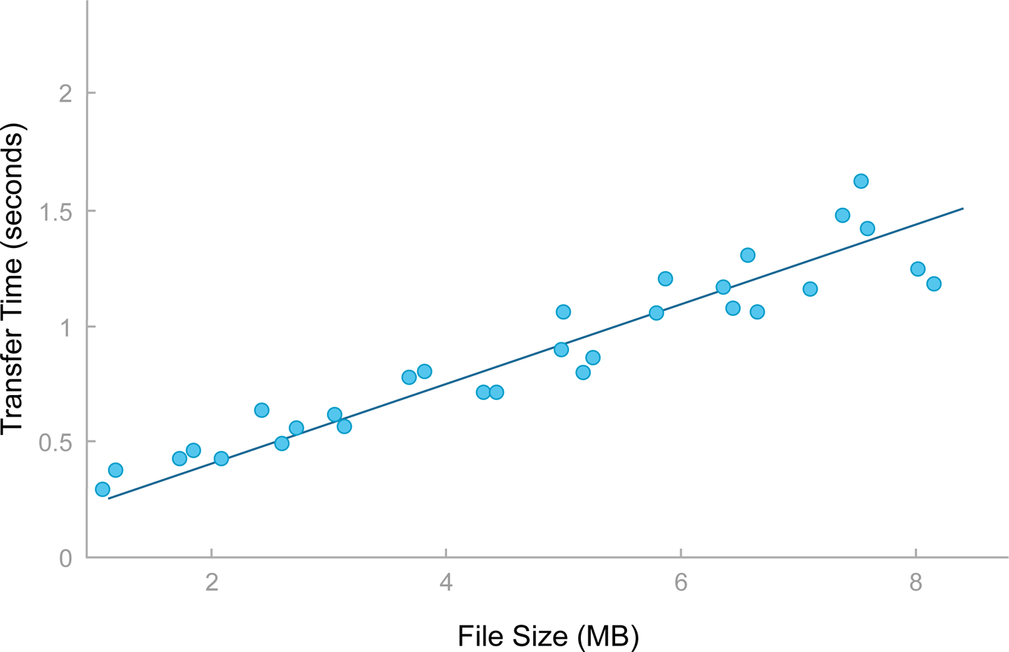
Figure 7-1. Detecting anomalies in the ML model

To train a linear regression ML model in SQL, you can use the following formula:

SELECT
covariance/variance as A,
mean_y - covariance/variance*mean_x AS B
FROM
(select sum(x*y)/count(*) - sum(x)/count(*)*sum(y)/count(*))
  as covariance,
(sum(x*x)/count(*) - sum(x)/count(*)*sum(x)/count(*))
  as variance,
sum(x)/count(*) as mean_x,
sum(y)/count(*) as mean_y from training_data) as t;

In this formula, x is the independent variable, and y is the variable we are trying to predict from x.

The statement outputs something similar to the following:

+--------------------+--------------------+
| A                  | B                  |
+--------------------+--------------------+
| 1.6000000000000012 | 0.6999999999999966 |
+--------------------+--------------------+

The values then can be used to predict another value of y from a value of x.

SELECT x, 1.6 * x + 0.69999
FROM data_to_predict;

It does not work well when the relationship is not linear between the inputs and the output. For example, the trajectory of airplanes after takeoff is nonlinear. The airplane accelerates, and the acceleration causes a nonlinear relationship between the input and the output variable (the prediction). For this type of model, you can use Polynomial regression to more accurately learn. Polynomial regression is a technique that learns the coefficients of a polynomial in the form y = ax + bx² + cx³ + … using labeled data. Polynomial regression can capture more complex behavior than linear regression. When the behavior the model is trying to predict becomes very complex, you can use regression trees.

Regression trees are a class of decision trees that produces a continuous output variable. They work by separating the domain, or the total possible range of inputs, into smaller domains. The inputs to a regression tree can be a mix of categorical and continuous variables, which then are combined.

Categorical: Classification

It is very often useful to determine if a data point can be matched to a known category, or class. Applications are very wide and range from rate prediction to face recognition. You can use multiple techniques to build ML models producing categorical variables.

K-NN, or K-Nearest-Neighbor, is a technique by which data is classified by directly comparing it with the labeled data. When a new data point needs to be classified, the new data point is compared with every labeled data point. The category from the labeled data points closest to the new data point is used as the output. In a real-time ML application, the newly classified point can be added to the labeled data in order to refine the model in real time.

To classify a point (x = 4, y = 2) using K-NN on a dataset in a table in a SQL database, you can use the following query:

SELECT
x, y, category,
sqrt( (x - 4)*(x-4) + (y-2)*(y-2) ) as distance
FROM
training_data_2
ORDER BY distance ASC
LIMIT 3;
+------+------+----------+--------------------+
| x    | y    | category | distance           |
+------+------+----------+--------------------+
|    2 |    4 | C        | 2.8284271247461903 |
|    1 |    2 | C        |                  3 |
|    3 |    5 | A        | 3.1622776601683795 |
+------+------+----------+--------------------+

In this case, two of the closest points have the category C, so picking C as the category would be a good choice.

When the data points have a large number of dimensions, it is more efficient to encode the data as vectors and to use a database that supports vector arithmetic. In a well-implemented database, vector arithmetic will be implemented using modern single instruction, multiple data (SIMD) instructions, allowing much more efficient processing. In this case, the sample query would look like this:

CREATE TABLE training_data_3 (category VARCHAR(5) PRIMARY KEY,
  vector VARBINARY(4096));

INSERT INTO training_data_3 (category, vector) SELECT 'A',
    json_array_pack('[3, 5, ...]');

SELECT
category,
EUCLEDIAN_DISTANCE(vector, json_array_pack('[4, 5, 23, ...]')
    as distance
FROM
training_data_3
ORDER BY distance ASC
LIMIT 3;

+----------+--------------------+
| category | distance           |
+----------+--------------------+
| C        | 2.8284271247461903 |
| C        |                  3 |
| A        | 3.1622776601683795 |
+----------+--------------------+

Determining Whether a Data Point Belongs to a Class by Using Logistic Regression

Logistic regression is a very common technique for categorical classification when the output can take only two values, “0” or “1.” It is commonly employed to predict whether an event will occur; for example, if a visitor to a web page will click an advertisement, or whether a piece of equipment is damaged, based on its sensor data. Logistic regression effectively learns a “threshold” in the input domain. The output value is 0 below the threshold and 1 above the threshold. You can train logistics regression online, allowing the model to be refined as predictions are made and as feedback comes in. When you need multiple thresholds to identify the category (e.g., if the input is between the values A and B, then “0”; otherwise “1”), you can use more powerful models such as decision trees and neural networks.

In practice, logistic regression often is used with large feature vectors that are most effectively represented as vectors, or strings of numbers. In the following example, the training of a logistic regression learns a weight vector w, and an intercept w_0. The trained model can be stored in a table in a database to allow online classification using logistic regression:

SELECT
 1/(1 + exp(-w_0 + dot_product(w,
  json_array_pack('[0, 0.1, 0.8, ...]')) as logistic_regression
FROM weight;

Continuous: Real-Time Clustering

Clustering is the task of grouping a set of data points into a group (called a cluster) such that each group consists of data points that are similar. A distance function determines the similarity between data points.

You can use the centroid-based clustering (k-means) technique to learn the center position of each cluster, called a centroid. To classify a data point, you compare it to each centroid, and assign it to the most similar centroid. When a data point is matched to a centroid, the centroid moves slightly toward the new data point. You can apply this technique to continuously update the clusters in real time, which is useful because it allows the model to constantly be updated to reflect new data points.

An example application of real-time clustering is to provide customized content recommendation, such as news articles or videos. Users and their viewing history are grouped into clusters. Recommendations can be given to a user by inspecting which videos the cluster watched that the user has not yet watched. Updating the clusters in real time allows those applications to react to changes in trends and provide up-to-date recommendations:

SELECT
cluster_name,
euclidean_distance(vector, json_array_pack('[1, 3, 5, ...]')
  as distance
FROM
clusters
ORDER BY distance ASC
LIMIT 1;
+--------------+--------------------+
| cluster_name | distance           |
+--------------+--------------------+
| cluster_1    | 2.8284271247461903 |
+--------------+--------------------+

Categorical: Real-Time Unsupervised Classification with Neural Networks

Neural networks are a very powerful tool to solve classification problems. They are composed of neurons, divided into layers. Typically, a neural network consists of an input layer, one or more hidden layers, and an output layer. Each layer uses the previous layer as an input. The final output layer would contain one neuron per possible category. The value of each output neuron determines whether an input belongs to a specific category. Image recognition is a good example of an application for neural networks. In those networks, the pixels of the image are fed in the neural network, and there is one output neuron for each object to be recognized. In the context of real-time ML, neural networks can be used to classify data points in real time. Neurons in the output layer can also be added in real time, in the context of unsupervised learning, to give the network the capacity to recognize an object it had not seen before, as illustrated in Figure 7-2.

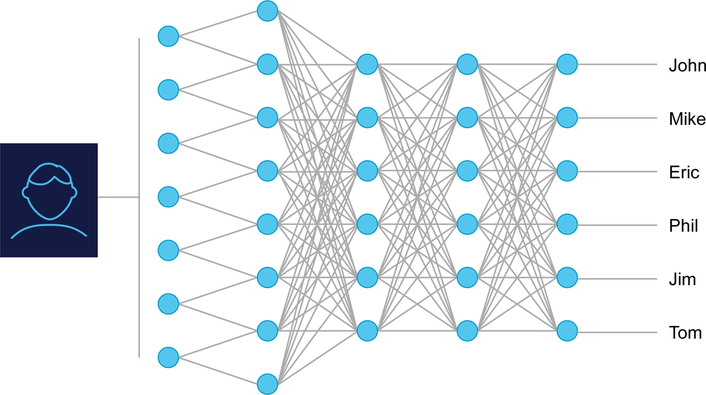
Figure 7-2. A neural network

The neurons of the output layer can be stored as vectors (one row/vector per output neuron) in a table. The following example illustrates how to evaluate the output layer of a neural network in a real-time database for facial recognition. We need to send a query to the database to determine which neurons in the output layer have a high output. The neurons with a high output determine which faces would match the input.

In the code example that follows, the output of the last hidden layer of the facial recognition neural network is passed in as a vector using json_array_pack:

SELECT
dot_product(neuron_vector,
  json_array_pack('[0, 0.4, 0.6 0,...]') as dot,
id
FROM
neurons
HAVING dot > 0.75;

You can use publicly available neural networks for facial recognition (one such example can be found at http://www.robots.ox.ac.uk/~vgg/software/vgg_face/).

Using a database to store the neurons provides the strong advantage that the model can be incrementally and transactionally updated concurrently with evaluation of the model. If no good match was found in the preceding example, the following code illustrates how to insert a neuron in the output layer to recognize this pattern if it were to come again:

INSERT INTO neurons (id, neuron_vector)
SELECT 'descriptor for this face',
  json_array_pack('[0, 0.4, 0.6 0,...]');

If the algorithm was to see the face again, it would know it has seen it before. This example demonstrates the role that infrastructure plays in allowing ML applications to operate in real time. There are countless ways in which you might implement a neural network for facial recognition, or any of the ML techniques discussed in this section. The examples have focused on pushing computation to a database in order to take advantage of distributed computation, data locality, and the power of SQL. The next chapter discusses considerations for building your application and data analytics stack on top of a distributed database.