Chapter 8. Building the Ideal Stack for Machine Learning
Building an effective machine learning (ML) pipeline requires balance between two natural but competing impulses. On one hand, you want to use existing software systems and libraries in order to move quickly and maximize performance. However, most likely there is not a preexisting piece of software that provides the exact utility you require. The competing impulse, then, is to eschew existing software tools and to build your system from scratch. The challenge is that this option requires greater expertise, is more time-consuming, and can ultimately be more expensive.
This tension echoes the classic “build versus buy” debate, which comes up at some stage of every business venture. ML is unique in that both extremes of the spectrum can seem reasonable in the appropriate light. For example, there are plenty of powerful analytics solutions on the market and you can probably get something off the ground without writing too much code. Conversely, at the end of the day ML is just math, not magic, and there is nothing stopping you from cracking a linear algebra textbook and starting from scratch. However, in the context of nearly any other engineering problem, both extremes raise obvious red flags. For example, if you are building a bridge, you would be skeptical if someone tried to sell you a one-size-fits-all bridge in a box. Similarly, it probably does not bode well for any construction project if you also plan to source and manufacture all the raw materials.
ML pipelines are not bridges, but should not be treated as totally dissimilar. As businesses further realize the promises of “big data,” ML pipelines take on a more central role as critical business infrastructure. As a result, ML pipelines demonstrate value not only by the accuracy of the models they employ, but the reliability, speed, and versatility of the system as a whole.
Example of an ML Data Pipeline
There is no limit to the number of different permutations of ML pipelines that a business can employ (not to mention different ways of rendering them graphically). This example focuses on a simple pipeline that employs a supervised learning model (classification or regression).
New Data and Historical Data
Figure 8-1 shows an ML pipeline applied to a real-time business problem. The top row of the diagram represents the operational component of the application, where the model is applied to automate real-time decision making. For instance, a user accesses a web page and the application must choose a targeted advertisement to display in the time it takes the page to load. When applied to real-time business problems, the operational component of the application always has restrictive latency requirement.

Figure 8-1. Data pipeline leading to real-time scoring
Model Training
The bottom row in Figure 8-1 represents the learning component of the application. It creates the model that the operational component applies to make decisions. Depending on the application, the training component might have less-stringent latency requirements because training is a one-time cost—scoring multiple data points does not require retraining. That being said, many applications can benefit from reduced training latency by enabling more frequent retraining as the dynamics of the underlying system change.
Scoring in Production
When we talk about supervised learning, we need to distinguish the way we think about scoring in development versus in production. Scoring latency in a development environment is generally just an annoyance. In production, the reduction or elimination of latency is a source of competitive advantage. This means that, when considering techniques and algorithms for predictive analytics, you need to evaluate not only the bias and variance of the model, but how the model will actually be used for scoring in production.
Scoring with supervised learning models presents another opportunity to push computation to a real-time database (Figure 8-2).

Figure 8-2. ML model expressed in SQL, computation pushed directly to database
Even though it can be tempting to perform scoring in the same interactive environment in which you developed the model, in most cases this will not satisfy the latency requirements of real-time use cases. Depending on the type of model, often the scoring function can be implemented in pure SQL. Then, instead of using separate systems for scoring and transaction processing, you do both in the database (Figure 8-3).
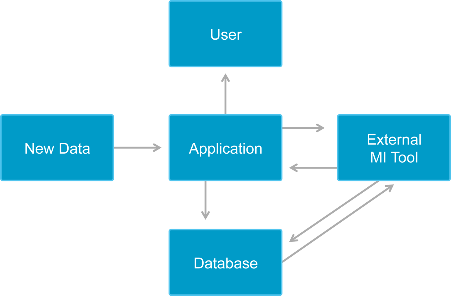
Figure 8-3. ML model expressed in an external tool, more data transfer and computation
Technologies That Power ML
The notion of a “stack” refers to the fact that there are generally several layers to any production software system. At the very least, there is an interface layer with which the users interact, and then there is the layer “below” that one that stores and manipulates the data that users access through the interface layer. In practice, an ML “stack” is not one dimensional. There is a production system that predicts, recommends, or detects anomalies, and makes this information available to end users, who might be customers or decision makers within an organization.
Adding data scientists, who build and modify the models that power the user-facing production system, adds another dimension to the “stack.” Depending on your interpretation of the stack metaphor, the tools used by a data scientist on a given day likely does not fit anywhere on the spectrum from “frontend” to “backend,” at least with respect to the user-facing production stack. However, there can, and often should, be overlap between the two toolchains.
Programming Stack: R, Matlab, Python, and Scala
When developing a model, data scientists generally work in a development environment tailored for statistics and ML like Python, R, Matlab, or Scala. These tools allow data scientists to train and test models all in one place and offer powerful abstractions for building models and making predictions while writing relatively little code. Every tool offers different features and performance characteristics suited to different tasks, but the good news is that your choice of development language likely will not make or break your project. Each of the tools discussed is extremely powerful and continually being improved. Figure 8-4 shows interactive data analysis in Python.
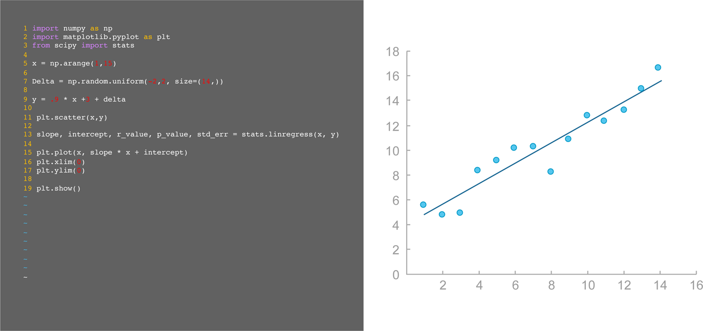
Figure 8-4. Interactive data analysis in Python
The programming languages and environments mentioned so far share (at least) one common design feature: interactivity. Each of these languages have Read-Evaluate-Print Loop (REPL) shell environments that allow the user to manipulate variables and functions interactively.
Beyond what they share, these languages fall into two general categories. R and Matlab (as well as SAS, Octave, and many others) are designed for numerical and statistical computation, modeling, data visualization, and ease of use for scientists and analysts who might not have a background in software engineering. The trade-off in design choices is that these are not general-purpose languages, and you generally do not write user-facing applications in them.
Python and Scala are more general-purpose languages, commonly used to write user-facing applications, in addition to being used interactively for data science. They share further characteristics in common, including support for both functional and object-oriented programming. While Python and Scala are relatively “high-level” languages, in that they do not require the programmer to delve too deeply into tricky areas like memory management and concurrency, both languages offer sufficiently good performance for many types of services and applications.
The popularity of infrastructure like Apache Kafka and Apache Spark contributed significantly to Scala’s growing prominence in recent years, whereas Python has been widely used at leading technology companies, including Google, for everything from web services to applications for managing distributed systems and datacenter resources.
Analytics Stack: Numpy/Scipy, TensorFlow, Theano, and MLlib
When building a new ML application, you should almost never start from scratch. If you wanted, you could spend a lifetime just building and optimizing linear algebra operators and completely lose sight of ML altogether, let alone any concrete business objective. For example, most ML libraries use at least some functionality from LAPACK, a numerical linear algebra library written in Fortran that has been used and continually improved since the 1970s.
The popular Python libraries Numpy and Scipy, for instance, both make calls out to LAPACK functions. In fact, these libraries make calls out to many external (non-Python) functions from libraries written in lower-level languages like Fortran or C. This is part of what make Python so versatile: in addition to offering an interpreter with good performance, it is relatively easy to call out to external libraries (and with relatively little overhead), so you get the usability of Python but the scientific computing performance of Fortran and C.
On the Scala side, adoption of Apache Spark has made the library MLlib widely used, as well. One of the biggest advantages of MLlib, and Spark more generally, is that programs execute in a distributed environment. Where many ML libraries run on a single machine, MLlib was always designed to run in a distributed environment.
Visualization Tools: Business Intelligence, Graphing Libraries, and Custom Dashboards
If it seems to you like there is an “abundance” of tools, systems, and libraries for data processing, there also might appear to be an overabundance of data visualization options. Lots of data visualization software, especially traditional business intelligence (BI), comes packaged with its own internal tools for data storage and processing. The trend more recently, as discussed in Chapter 5, is toward “thinner” clients for visualization and pushing more computation to databases and other “backend” systems. Many of the most widely used BI tools now provide a web interface.
Widespread adoption of HTML5, with features like Canvas and SVG support, and powerful JavaScript engines like Google’s V8 and Mozilla’s SpiderMonkey have transformed the notion of what can and should run in the browser. Emscripten, an LLVM-to-JavaScript, enables you to translate, for instance, C and C++ programs into extremely optimized JavaScript programs. WebAssembly is a low-level bytecode that makes it possible to create more expressive programming and more efficient execution of JavaScript now, and whatever JavaScript becomes or is replaced by in the future.
There is an interesting, and not coincidental, parallel between the advances in web and data processing technologies: both have been changed dramatically by low-level languages that enable new, faster methods of code compilation that preserve or even improve the efficiency of the compiled program versus old methods. When your database writes and compiles distributed query execution plans, and you can crunch the final numbers with low-level, optimized bytecode in the browser, there is less need for additional steps between the browser and your analytics backend.
Top Considerations
As with any production software system, success in deploying ML models depends, over time, on know-how and familiarity with your own system. The following sections will cover specific areas to focus on when designing and monitoring ML and data processing pipelines.
Ingest Performance
It might seem odd to mention ingest as a top consideration given that training ML models is frequently done offline. However, there are many reasons to care about ingest performance, and you want to avoid choosing a tool early on in your building process that prevents you from building a real-time system later on. For instance, Hadoop Distributed File System (HDFS) is great for cheaply storing enormous volumes of data, and it works just fine as a data source for a data scientist developing a model. That being said, it is not designed for executing queries and ingesting data simultaneously and would likely not be the ideal datastore for a real-time analytics platform. By starting out with the proper database or data warehouse, you prepare yourself to build a versatile platform that powers applications, serves data scientists, and can mix analytics with ingest and data processing workloads.
Analytics Performance
In addition to considering performance while ingesting data, you also should think about “pure” analytics performance, namely how quickly can the system execute a query or job. Analytics performance is a function of the system’s ability to generate and optimize a plan, and then to execute that plan efficiently. A good execution plan will minimize the amount of data that needs to be scanned and transferred and might be the product of logical query “rewrites” that transform the user’s query into a logically equivalent query that reduces computation or another resource.
In addition, databases designed for analytics performance implement a number of optimizations allowing them to speed up analytical queries. Modern databases implement a column-store engine, which lays out the data one column at a time rather than one row at a time. This has a number of benefits: first, it allows the data to be efficiently compressed by using the properties of the column. For example, if a VARCHAR(255) column only takes a few distinct values, the database will compress the column by using dictionary encoding and will only store the index of the value in the dictionary rather than the full value. This reduces the size of the data and reduces the input/output (I/O) bandwidth required to process data in real time. Further, this data layout allows a well-implemented columnar engine to take advantage of modern single instruction, multiple data (SIMD) instructions sets. This enables the database to process multiple rows per clock cycles of the microprocessor, as demonstrated in Figure 8-5.

Figure 8-5. Scalar versus SIMD computation
The AVX2 instruction set, present on most modern Intel microprocessors, is used by modern databases to speed up the scanning of data, the filtering of data, and the aggregation of data. The following query is a good example of a query benefiting heavily from a well-optimized columnar engine running on a microprocessor supporting the AVX2 instruction set:
SELECT key, COUNT(*) as count FROM table t GROUP BY key;
When the number of distinct values of “key” is small, a modern data warehouse needs as little as two clock cycles for each record processed. As such, it is recommended to use microprocessors supporting those instructions sets in your real-time analytics stack.
Distributed Data Processing
This chapter’s final topic has been touched on previously, but bears repeating. In many cases, distributed data processing is crucial to building real-time applications. Although many ML algorithms are not (or not easily) parallelizable, this is only a single step in your pipeline. Distributed message queues, databases, data warehouses, and many other data processing systems are now widely available and, in many cases, the industry standard. If there is any chance that you will need to scale a particular step in a data pipeline, it is probably worth it to begin by using a distributed, fault-tolerant system for that step.