Scalable BI

The size of datasets and the tools needed to process them has exceeded what can be done on a single machine. Even when operating on a dataset that can fit on a laptop hard drive, this might not be the most efficient way of accessing information. Transferring large amounts of data over a network adds latency. In addition, BI tools are generally designed to work with databases, and the BI datastores themselves might not be equipped to handle especially large datasets (Figure 5-1).

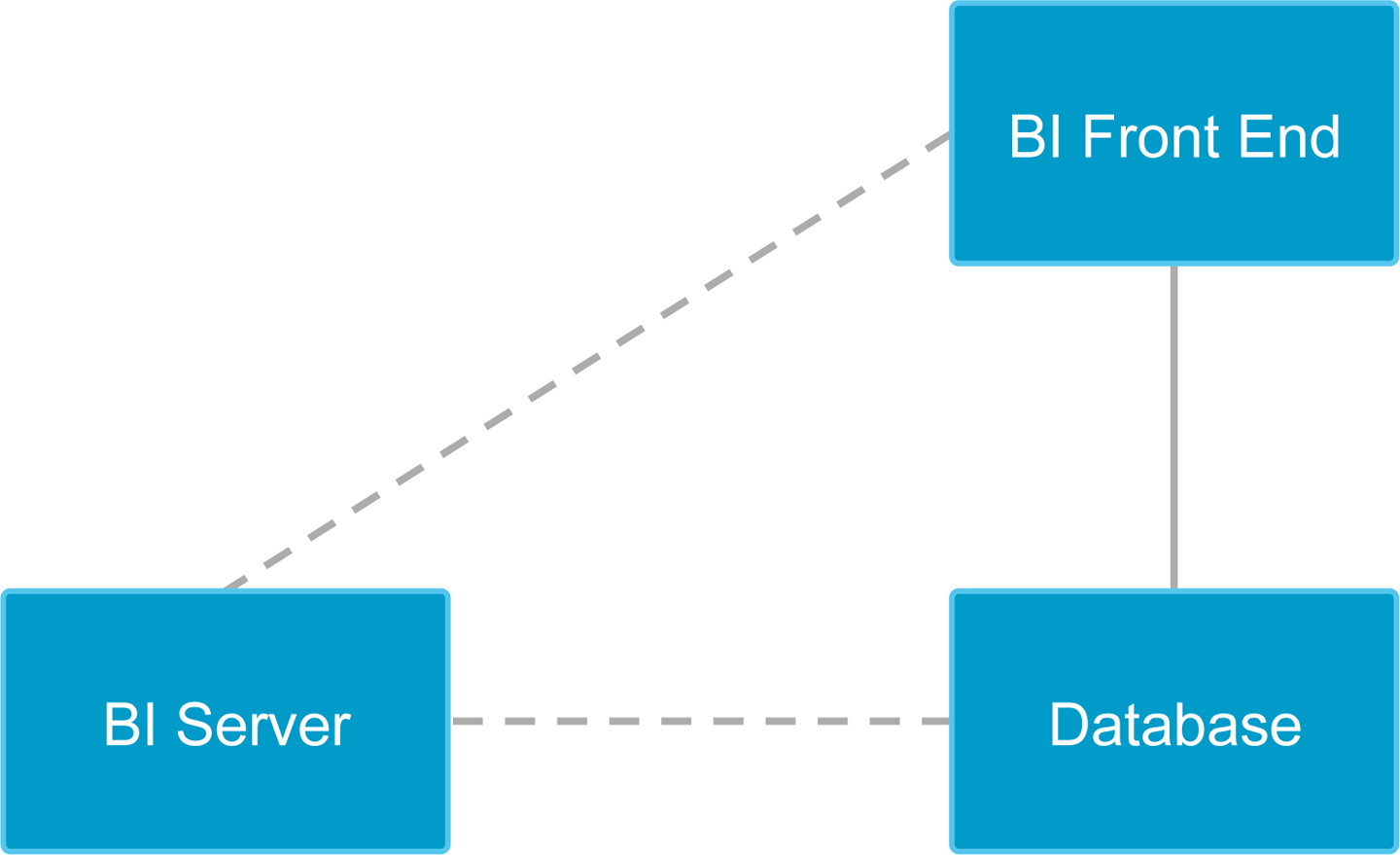
Figure 5-1. Typical BI architecture

Many modern BI tools employ a “thin” client, through which an analyst can run queries and generate diagrams and reports. Increasingly, these BI clients run in a web browser. The client is “thin” in the sense that it serves primarily as a user interface, and the user’s queries “pass through” to a separate BI server or directly to a database.

Query Optimization for Distributed Data Warehouses

One of the core technologies in a distributed data warehouse is distributed query execution. How the database draws up and runs a query execution plan makes or breaks fast query response times. The plan is a sequence of suboperations that the database will go through in order to process a query as a whole and return a result.

All databases do some query planning, but it takes on much greater importance in a distributed system. The plan, for instance, determines which and how much data needs to be transferred between machines, which can be, and often is, the primary bottleneck in distributed query execution.

Example 5-1 shows a query optimization done by a distributed database. The sample query is based on one from a well-known database benchmark called TPC-H. After the initial query, which would be supplied by a user or an application, everything else happens within the database. Although this discussion is intended for a more technical audience, all readers are encouraged to at least skim the example to appreciate how much theory goes into distributed query optimization. If nothing else, this example should demonstrate the value of a database with a good optimizer and distributed query execution!

SELECT Sum(l_extendedprice) / 7.0 AS avg_yearly
FROM   lineitem,
       part
WHERE  p_partkey = l_partkey
       AND p_brand = 'Brand#43'
       AND p_container = 'LG PACK'
       AND l_quantity < (SELECT 0.2 * Avg(l_quantity)
                         FROM   lineitem
                         WHERE  l_partkey = p_partkey)

Example 5-1 demonstrates running the query on two tables, part and lineitem, that are partitioned along the columns p_partkey and l_orderkey, respectively.

This query computes the average annual revenue that would be lost if the company were to stop filling small orders of certain parts. The query is (arguably) written in a way that makes intuitive sense to an analyst: compute the sum of prices of parts from some brand, in some bin, where the quantity sold is less than the result of a subquery. The subquery computes the average quantity of the part that is sold and then multiplies by .2.

This version of the query, although readable, likely will not execute efficiently without some manipulation. You may recall that part and lineitem are partitioned on p_partkey and l_orderkey, but the query is joining on p_partkey = l_partkey, where l_partkey is not a shard key. The subquery is “correlated” on p_partkey, meaning that the subquery does not actually select from part, and the p_partkey in the inner query refers to the same p_partkey from the outer query. Because the correlating condition of the inner query joins on a nonshard key, there are two (naive) options: first, you could trigger a remote query for every line of part that is scanned (very bad idea); or you could repartition lineitem on l_partkey. However, lineitem represents a large fact table, so repartitioning the entire table would be very expensive (time-consuming). Neither option is attractive.

Fortunately, there is an alternative. The optimizers of modern databases contain a component that rewrites SQL queries into other SQL queries that are logically equivalent, but easier for the database to execute in practice. Example 5-2 shows how a database might rewrite the query from Example 5-1.

SELECT Sum(l_extendedprice) / 7.0 AS avg_yearly
FROM   lineitem,
       (SELECT 0.2 * Avg(l_quantity) AS s_avg,
               l_partkey             AS s_partkey
        FROM   lineitem,
               part
        WHERE  p_brand = 'Brand#43'
               AND p_container = 'LG PACK'
               AND p_partkey = l_partkey
        GROUP  BY l_partkey) sub
WHERE  s_partkey = l_partkey
       AND l_quantity < s_avg

This rewritten query is logically equivalent to the one shown in Example 5-1, which is to say that it can prove that the two queries will always return the same result regardless of the underlying data. The latter formulation rewrites what was originally a join between two tables into a join between a table and a subquery, for which the outer query depends on the “inner” subquery. The advantage of this rewrite is that the inner query can execute first and return a small enough result that it can be “broadcast” across the cluster to the other nodes. The problem with the naive executions of the query from Example 5-1 is that it either requires moving too much data because lineitem is a fact table and would need to be repartitioned, or required executing too many subqueries, because the correlating condition did not match the sharding pattern. The formulation in Example 5-2 circumvents these problems because the subquery filters a smaller table (part) and then inexpensively joins it with a larger table (lineitem) by broadcasting the filtered results from the smaller table and only “seeking into” the larger table when necessary. In addition, the GROUP BY can be performed in parallel. The result of the subquery is itself small and can be broadcast to execute the join with lineitem in the outer query.

Example 5-3 explains the entire process more precisely.

Project [s2 / 7.0 AS avg_yearly]
Aggregate [SUM(1) AS s2]
Gather partitions:all
Aggregate [SUM(lineitem_1.l_extendedprice) AS s1]
Filter [lineitem_1.l_quantity < s_avg]
NestedLoopJoin
|---IndexRangeScan lineitem AS lineitem_1,
| KEY (l_partkey) scan:[l_partkey = p_partkey]
Broadcast
HashGroupBy [AVG(l_quantity) AS s_avg]
groups:[l_partkey]
NestedLoopJoin |---IndexRangeScan lineitem,
| KEY (l_partkey) scan:[l_partkey = p_partkey]
Broadcast
Filter [p_container = 'LG PACK' AND p_brand = 'Brand#43']
TableScan part, PRIMARY KEY (p_partkey)

Again, there is no need to worry if you do not understand every step of this query rewriting and planning process. Distributed query optimization is an area of active research in computer science, and it is not reasonable to expect business analysts or even most software engineers to be experts in this area. One of the advantages of a distributed SQL database with a good optimizer and query planner is that users do not need to understand the finer points of distributed query execution, but they can still reap the benefits of distributed computing.

Scale-Out Architecture

As your analytics infrastructure grows more sophisticated, the amount of data that it both generates and captures will increase dramatically. For this reason, it is important to build around distributed systems with scale-out architectures.

Columnstore Query Execution

A columnstore is a class of database that employs a modern, analytics-friendly storage format that stores columns, or segments of columns, together on the storage medium. This allows for faster columns scans and aggregations. In addition, some databases will store metadata about the contents of column segments to help with even more efficient data scanning. For example, a columnstore database can store metadata like the minimum and maximum values in a column segment. Then, when computing a query with a WHERE condition involving values in that column, the database can use the column segment metadata to determine whether to “open up” a column segment to search for matching data inside, or whether to skip over the column segment entirely.

Intelligent Data Distribution

Although distributed computing can speed up data processing, a poorly designed system can negate or even invert the performance benefits of having multiple machines. Parallelism adds CPUs, but many of those CPUs are on separate machines, connected by a network. Efficient distribution of data makes it possible to manage concurrent workloads and limit bottlenecks.

Rise of Data Capture for Analytics

In a short span, entire industries have been born that didn’t exist previously. Each of these areas is supported by one or more of the world’s largest companies:

• App stores from Apple and Google

• Online music, video, and books: Apple, Google, and Amazon

• Seller marketplaces from Amazon.com

• Social networks from Facebook

Each of these services share a couple of common characteristics that drive their data processing workloads:

• Incredibly large end-user bases, numbering hundreds of millions

• A smaller (but still large) base of creators or sellers

These businesses provide analytics for a variety of audiences including content providers, advertisers, and end users, as well as many within the company itself, including product managers, business analysts, and executives. All of these characteristics culminate in a stack that starts with the platform provider, extends up to the creators or sellers, and ends with consumers. At each level, there is a unique analytics requirement.

App Store Example

Some of the aforementioned large, successful companies do significant business through digital commerce platforms known as app stores. We will use app stores as an example to explore analytics architectures across this type of stack. App stores are also an ideal example of new workloads that require a fresh approach to data engineering.

The largest app stores share the following characteristics:

• Hundreds of millions of end users

• Millions of application developers

• Dozens of app segments

• One primary platform provider (e.g., Apple, Google)

In addition, the backend data systems powering the largest app stores process many types of data:

• The distribution of apps to end users

• App data coming from each app from each end user

• Transactional data

• Log data

All of these different types of data from a platform with many users results in large and rapidly growing datasets. Managing and making sense of these large data volumes requires the following capabilities:

Low-latency query execution

Even when the data is not “new,” query execution latency determines the speed of analytics applications and dramatically affects the speed and productivity of data scientists.

High concurrency

Data systems with many users can become bogged down if it does not manage concurrency well. As with query execution, concurrency can affect the performance of both applications and data scientists.

Fast data capture

In the interest of unifying historical with real-time analytics, it is crucial that your database have good ingest speed. Even for systems that do not yet incorporate real-time operations, fast data ingest saves both time and compute resources that can be dedicated to other analytics processes.

The final point, fast data capture, might seem unusual in the context of a discussion about historical data. However, the capability enables you to unify analytics on historical data with the real-time systems that power your business. Whether you subscribe to the metaphors of lakes or warehouses, building intelligent real-time applications requires rethinking the role historical data plays in shaping business decisions. Historical data itself might not be changing, but the applications, powered by models built using historical data, will create data that needs to be captured and analyzed. Moreover, new historical data is created every second your business operates. With these concerns in mind, we need another data architecture metaphor that conveys constant movement of data.