19

TensorFlow 2 Ecosystem

In this chapter, we will learn about the different components of the TensorFlow ecosystem. The chapter will elaborate upon TensorFlow Hub – a repository for pretrained deep learning models – and TensorFlow Datasets – a collection of ready-to-use datasets for ML tasks. TensorFlow JS, the solution for training and deploying ML models on the web, will be introduced. We will also learn about TensorFlow Lite, an open-source deep learning framework for mobile and edge devices. Some examples of Android, iOS, and Raspberry Pi applications will be discussed, together with examples of deploying pretrained models such as MobileNet v1, v2, v3 (image classification models designed for mobile and embedded vision applications), PoseNet for pose estimation (a vision model that estimates the poses of people in image or video), DeepLab segmentation (an image segmentation model that assigns semantic labels (for example, dog, cat, and car) to every pixel in the input image), and MobileNet SSD object detection (an image classification model that detects multiple objects with bounding boxes). The chapter will conclude with an example of federated learning, a decentralized machine learning framework that is thought to respect user privacy. The chapter includes:

• TensorFlow Hub
• TensorFlow Datasets
• TensorFlow Lite and using it for mobile and edge applications
• Federated learning at edge
• TensorFlow JS
• Using Node.js with TensorFlow models

Let’s begin with TensorFlow Hub.

TensorFlow Hub

Even if you have a powerful computer, training a machine learning model can take days or weeks. And once you’ve trained the model, deploying it to different devices can be difficult and time-consuming. Depending upon the platform you want to deploy, you might need it in different formats.

You can think of TensorFlow Hub as a library with many pretrained models. It contains hundreds of trained, ready-to-deploy deep learning models. TensorFlow Hub provides pretrained models for image classification, image segmentation, object detection, text embedding, text classification, video classification and generation, and much more. The models in TF Hub are available in SavedModel, TFLite, and TF.js formats. We can use these pretrained models directly for inference or fine-tune them. With its growing community of users and developers, TensorFlow Hub is the go-to place for finding and sharing machine learning models. To use TensorFlow Hub, we first need to install it:

pip install tensorflow_hub

Once installed, we can import it simply using:

import tensorflow_hub as hub

and load the model using the load function:

model = hub.load(handle)

Here handle is a string, which contains the link of the model we wants to use. If we want to use it as part of our existing model, we can wrap it as a Keras layer:

hub.KerasLayer(
    handle,
    trainable=False,
    arguments=None,
    _sentinel=None,
    tags=None,
    signature=None,
    signature_outputs_as_dict=None,
    output_key=None,
    output_shape=None,
    load_options=None,
    **kwargs
)

By changing the parameter trainable to True, we can fine-tune the model for our specific data.

Figure 19.1 shows the easy-to-use web interface to select different models at the tfhub.dev site. Using the filters, we can easily find a model to solve our problem.

We can choose which type and format we need, as well as who published it!

Figure 19.1: The tfhub.dev site showing different filters

Using pretrained models for inference

Let us see how you can leverage pretrained models from TensorFlow Hub. We will consider an example of image classification:

1. Let us import the necessary modules:

   import tensorflow as tf
   import tensorflow_hub as hub
   import requests
   from PIL import Image
   from io import BytesIO
   import matplotlib.pyplot as plt
   import numpy as np
   
2. We define a function for loading an image from a URL. The functions get the image from the web, and we reshape it by adding batch indexes for inference. Also, the image is normalized and resized according to the pretrained model chosen:

   def load_image_from_url(img_url, image_size):
     """Get the image from url. The image return has shape [1, height, width, num_channels]."""
     response = requests.get(img_url, headers={'User-agent': 'Colab Sample (https://tensorflow.org)'})
     image = Image.open(BytesIO(response.content))
     image = np.array(image)
     # reshape image
     img_reshaped = tf.reshape(image, [1, image.shape[0], image.shape[1], image.shape[2]]) 
     # Normalize by convert to float between [0,1]
     image = tf.image.convert_image_dtype(img_reshaped, tf.float32) 
     image_padded = tf.image.resize_with_pad(image, image_size, image_size)
     return image_padded, image
   
3. Another helper function to show the image:

   def show_image(image, title=''):
     image_size = image.shape[1]
     w = (image_size * 6) // 320
     plt.figure(figsize=(w, w))
     plt.imshow(image[0], aspect='equal')
     plt.axis('off')
     plt.title(title)
     plt.show()
   
4. The model we are using is EfficientNet-B2 (https://arxiv.org/abs/1905.11946) trained on the ImageNet dataset. It gives better accuracy, is smaller in size, and gives faster inference. For convenience, we choose images to be resized to 330 x 330 pixels. We use the helper function defined in step 2 to download the image from Wikimedia:

   image_size = 330
   print(f"Images will be converted to {image_size}x{image_size}")
   img_url =  "https://upload.wikimedia.org/wikipedia/commons/c/c6/Okonjima_Lioness.jpg"
   image, original_image = load_image_from_url(img_url, image_size) 
   show_image(image, 'Scaled image')
   

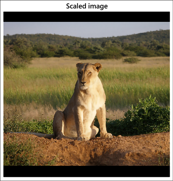
Figure 19.2: The image taken from the web for classification, scaled to size 330 x 330 pixels

5. For completeness, we also get all the labels of ImageNet data so that we can infer the label from the model prediction; we download it from a public repository of TensorFlow:

   labels_file = "https://storage.googleapis.com/download.tensorflow.org/data/ImageNetLabels.txt"
   #download labels and creates a maps
   downloaded_file = tf.keras.utils.get_file("labels.txt", origin=labels_file)
   classes = []
   with open(downloaded_file) as f:
     labels = f.readlines()
     classes = [l.strip() for l in labels]
   
6. Now that all the ingredients are ready, we download the model from tfhub.dev:

   classifier = hub.load("https://tfhub.dev/tensorflow/efficientnet/b2/classification/1")
   
7. We get the softmax probabilities for all the classes for the image downloaded in step 5:

   probabilities = tf.nn.softmax(classifier(image)).numpy()
   
8. Let us see the top prediction:

   top_5 = tf.argsort(probabilities, axis=-1, direction="DESCENDING")[0][:5].numpy()
   show_image(image, f'{classes[top_5[0]+1]}: {probabilities[0][top_5][0]:.4f}')
   

Figure 19.3: The image with the label prediction of lion

So, as we can see, in a few lines of code we get a perfect inference – the image is of a lioness, and the closest label for it in the ImageNet dataset is that of a lion, which the model has correctly predicted. By using the pretrained models of TF Hub, we can focus on our product workflow, and get better models and faster production.

TensorFlow Datasets

TensorFlow Datasets (TFDS) is a powerful tool for anyone working with machine learning. It provides a collection of ready-to-use datasets that can be easily used with TensorFlow or any other Python ML framework. All datasets are exposed as tf.data.Datasets, making it easy to use them in your input pipeline.

With TFDS, you can quickly get started with your machine learning projects and save time by not having to collect and prepare your own data. The library currently contains a wide variety of datasets, including image classification, object detection, text classification, and more. In addition, the library provides tools for creating new datasets from scratch, which can be useful for researchers or developers who need to create custom datasets for their own projects. TFDS is open source and released under the Apache 2.0 license. To be able to use TFDS, you will need to install it:

pip install tensorflow-datasets

Once installed, you can import it as:

import tensorflow_datasets as tfds

At the time of writing this book, TFDS contained 224 public datasets for a large range of tasks:

datasets = tfds.list_builders()
print(f"TFDS contains {len(datasets)} datasets")

### Output
TFDS contains 224 datasets

In this section, we will introduce you to TFDS and show how it can simplify your training process by exploring its underlying structure as well as providing some best practices for loading large amounts into machine learning models efficiently.

Load a TFDS dataset

Each dataset in TFDS is identified by its unique name, and associated with each dataset is also a publisher and dataset version. To get the data, you can use the TFDS load function (it is a powerful function with a lot of flexibility; you can read more about the function at https://www.tensorflow.org/datasets/api_docs/python/tfds/load):

tfds.load(
    name: str,
    *,
    split: Optional[Tree[splits_lib.SplitArg]] = None,
    data_dir: Optional[str] = None,
    batch_size: tfds.typing.Dim = None,
    shuffle_files: bool = False,
    download: bool = True,
    as_supervised: bool = False,
    decoders: Optional[TreeDict[decode.partial_decode.DecoderArg]] =
None,
    read_config: Optional[tfds.ReadConfig] = None,
    with_info: bool = False,
    builder_kwargs: Optional[Dict[str, Any]] = None,
    download_and_prepare_kwargs: Optional[Dict[str, Any]] = None,
    as_dataset_kwargs: Optional[Dict[str, Any]] = None,
    try_gcs: bool = False
)

You only need to specify the dataset name; the rest of the parameters are optional. You can read more about the optional arguments from TFDS docs. For example, below, we are downloading the famous MNIST dataset:

data, info = tfds.load(name="mnist", as_supervised=True, split=['train', 'test'], with_info=True)

The preceding statement downloads both the training and test dataset of MNIST into the variable data. Since the as_supervised flag is set to True, the labels are downloaded with the data, and the detailed information about the dataset is downloaded in info.

Let us first check the info:

print(info)

### output
tfds.core.DatasetInfo(
    name='mnist',
    version=3.0.1,
    description='The MNIST database of handwritten digits.',
    homepage='http://yann.lecun.com/exdb/mnist/',
    features=FeaturesDict({
        'image': Image(shape=(28, 28, 1), dtype=tf.uint8),
        'label': ClassLabel(shape=(), dtype=tf.int64, num_classes=10),
    }),
    total_num_examples=70000,
    splits={
        'test': 10000,
        'train': 60000,
    },
    supervised_keys=('image', 'label'),
    citation="""@article{lecun2010mnist,
      title={MNIST handwritten digit database},
      author={LeCun, Yann and Cortes, Corinna and Burges, CJ},
      journal={ATT Labs [Online]. Available: http://yann.lecun.com/exdb/mnist},
      volume={2},
      year={2010}
    }""",
    redistribution_info=,
)

So, we can see that the information is quite extensive. It tells us about the splits and the total number of samples in each split, the keys available if used for supervised learning, the citation details, and so on. The variable data here is a list of two TFDS dataset objects – the first one corresponding to the test dataset and the second one corresponding to the train dataset. TFDS dataset objects are dict by default. Let us take one single sample from the train dataset and explore:

data_train = data[1].take(1)
for sample, label in data_train:
  print(sample.shape)
  print(label)

### output
(28, 28, 1)
tf.Tensor(2, shape=(), dtype=int64)

You can see that the sample is an image of handwritten digits of the shape 28 x 28 x 1 and its label is 2. For image data, TFDS also has a method show_examples, which you can use to view the sample images from the dataset:

fig = tfds.show_examples(data[0], info)

Figure 19.4: Sample from test dataset of MNIST dataset

Building data pipelines using TFDS

Let us build a complete end-to-end example using the TFDS data pipeline:

1. As always, we start with importing the necessary modules. Since we will be using TensorFlow to build the model, and TFDS for getting the dataset, we are including only these two for now:

   import tensorflow as tf
   import tensorflow_datasets as tfds
   
2. Using the Keras Sequential API, we build a simple convolutional neural network with three convolutional layers and two dense layers:

   model = tf.keras.models.Sequential([ 
     tf.keras.layers.Conv2D(16, (3,3), activation='relu', input_shape=(300, 300, 3)), 
     tf.keras.layers.MaxPooling2D(2, 2),
     tf.keras.layers.Conv2D(32, (3,3), activation='relu'), 
     tf.keras.layers.MaxPooling2D(2,2), 
     tf.keras.layers.Conv2D(64, (3,3), activation='relu'), 
     tf.keras.layers.MaxPooling2D(2,2), 
     tf.keras.layers.Flatten(), 
     tf.keras.layers.Dense(256, activation='relu'), 
     tf.keras.layers.Dense(1, activation='sigmoid')
   ])
   
3. We will be building a binary classifier, so we choose binary cross entropy as the loss function, and Adam as the optimizer:

   model.compile(optimizer='Adam', loss='binary_crossentropy',metrics=['accuracy'])
   
4. Next, we come to the dataset. We are using the horses_or_humans dataset, so we use the tfds.load function to get the training and validation data:

   data = tfds.load('horses_or_humans', split='train', as_supervised=True) 
   val_data = tfds.load('horses_or_humans', split='test', as_supervised=True)
   
5. The images need to be normalized; additionally, for better performance, we will augment the images while training:

   def normalize_img(image, label):
     """Normalizes images: 'uint8' -> 'float32'."""
     return tf.cast(image, tf.float32) / 255., label
   def augment_img(image, label):
     image, label = normalize_img(image, label)
     image = tf.image.random_flip_left_right(image)
     return image, label
   
6. So now we build the pipeline; we start with cache for better memory efficiency, apply the pre-processing steps (normalization and augmentation), ensure that data is shuffled while training, define the batch size, and use prefetch so that the next batch is brought in as the present batch is being trained on. We repeat the same steps for the validation data. The difference is that validation data need not be augmented or shuffled:

   data = data.cache()
   data = data.map(augment_img, num_parallel_calls=tf.data.AUTOTUNE)
   train_data = data.shuffle(1024).batch(32)
   train_data = train_data.prefetch(tf.data.AUTOTUNE)
   val_data = val_data.map(normalize_img, num_parallel_calls=tf.data.AUTOTUNE)
   val_data = val_data.batch(32)
   val_data = val_data.cache()
   val_data = val_data.prefetch(tf.data.AUTOTUNE)
   
7. And finally, we train the model:

   %time history = model.fit(train_data, epochs=10, validation_data=val_data, validation_steps=1)
   

Play around with different parameters of the data pipeline and see how it affects the training time. For example, try removing prefetch and cache and not specifying num_parallel_calls.

TensorFlow Lite

TensorFlow Lite is a lightweight platform designed by TensorFlow. This platform is focused on mobile and embedded devices such as Android, iOS, and Raspberry Pi. The main goal is to enable machine learning inference directly on the device by putting a lot of effort into three main characteristics: (1) a small binary and model size to save on memory, (2) low energy consumption to save on the battery, and (3) low latency for efficiency. It goes without saying that battery and memory are two important resources for mobile and embedded devices. To achieve these goals, Lite uses a number of techniques such as quantization, FlatBuffers, mobile interpreter, and mobile converter, which we are going to review briefly in the following sections.

Quantization

Quantization refers to a set of techniques that constrains an input made of continuous values (such as real numbers) into a discrete set (such as integers). The key idea is to reduce the space occupancy of Deep Learning (DL) models by representing the internal weight with integers instead of real numbers. Of course, this implies trading space gains for some amount of performance of the model. However, it has been empirically shown in many situations that a quantized model does not suffer from a significant decay in performance. TensorFlow Lite is internally built around a set of core operators supporting both quantized and floating-point operations.

Model quantization is a toolkit for applying quantization. This operation is applied to the representations of weights and, optionally, to the activations for both storage and computation. There are two types of quantization available:

• Post-training quantization quantizes weights and the result of activations post-training.
• Quantization-aware training allows for the training of networks that can be quantized with minimal accuracy drop (only available for specific CNNs). Since this is a relatively experimental technique, we are not going to discuss it in this chapter, but the interested reader can find more information in [1].

TensorFlow Lite supports reducing the precision of values from full floats to half-precision floats (float16) or 8-bit integers. TensorFlow reports multiple trade-offs in terms of accuracy, latency, and space for selected CNN models (see Figure 19.5, source: https://www.tensorflow.org/lite/performance/model_optimization):

Figure 19.5: Trade-offs for various quantized CNN models

FlatBuffers

FlatBuffers (https://google.github.io/flatbuffers/) is an open-source format optimized to serialize data on mobile and embedded devices. The format was originally created at Google for game development and other performance-critical applications. FlatBuffers supports access to serialized data without parsing/unpacking for fast processing. The format is designed for memory efficiency and speed by avoiding unnecessary multiple copies in memory. FlatBuffers works across multiple platforms and languages such as C++, C#, C, Go, Java, JavaScript, Lobster, Lua, TypeScript, PHP, Python, and Rust.

Mobile converter

A model generated with TensorFlow needs to be converted into a TensorFlow Lite model. The converter can introduce optimizations for improving the binary size and performance. For instance, the converter can trim away all the nodes in a computational graph that are not directly related to inference but instead are needed for training.

Mobile optimized interpreter

TensorFlow Lite runs on a highly optimized interpreter that is used to optimize the underlying computational graphs, which in turn are used to describe the machine learning models. Internally, the interpreter uses multiple techniques to optimize the computational graph by inducing a static graph order and by ensuring better memory allocation. The interpreter core takes ~100 kb alone or ~300 kb with all supported kernels.

Supported platforms

On Android, the TensorFlow Lite inference can be performed using either Java or C++. On iOS, TensorFlow Lite inference can run in Swift and Objective-C. On Linux platforms (such as Raspberry Pi), inferences run in C++ and Python. TensorFlow Lite for microcontrollers is an experimental port of TensorFlow Lite designed to run machine learning models on microcontrollers based on Arm Cortex-M (https://developer.arm.com/ip-products/processors/cortex-m) and series processors, including Arduino Nano 33 BLE Sense (https://store.arduino.cc/nano-33-ble-sense-with-headers), SparkFun Edge (https://www.sparkfun.com/products/15170), and the STM32F746 Discovery kit (https://www.st.com/en/evaluation-tools/32f746gdiscovery.html). These microcontrollers are frequently used for IoT applications.

Architecture

The architecture of TensorFlow Lite is described in Figure 19.6 (from https://www.tensorflow.org/lite/convert/index). As you can see, both tf.keras (for example, TensorFlow 2.x) and low-Level APIs are supported. A standard TensorFlow 2.x model can be converted by using TFLite Converter and then saved in a TFLite FlatBuffer format (named .tflite), which is then executed by the TFLite interpreter on available devices (GPUs and CPUs) and on native device APIs. The concrete function in Figure 19.6 defines a graph that can be converted to a TensorFlow Lite model or be exported to a SavedModel:

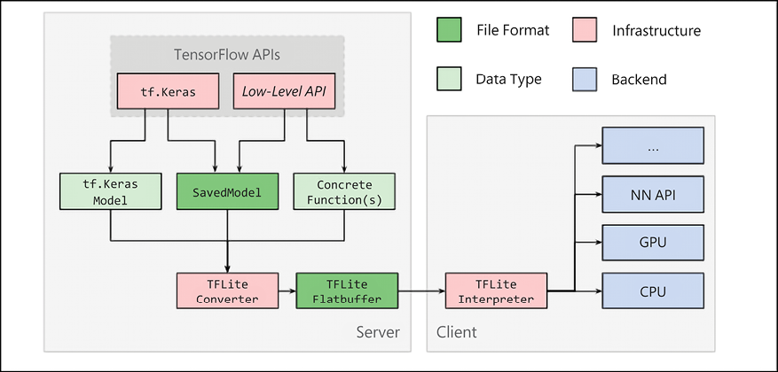
Figure 19.6: TensorFlow Lite internal architecture

Using TensorFlow Lite

Using TensorFlow Lite involves the following steps:

1. Model selection: A standard TensorFlow 2.x model is selected for solving a specific task. This can be either a custom-built model or a pretrained model.
2. Model conversion: The selected model is converted with the TensorFlow Lite converter, generally invoked with a few lines of Python code.
3. Model deployment: The converted model is deployed on the chosen device, either a phone or an IoT device, and then run by using the TensorFlow Lite interpreter. As discussed, APIs are available for multiple languages.
4. Model optimization: The model can be optionally optimized by using the TensorFlow Lite optimization framework.

A generic example of an application

In this section, we are going to see how to convert a model to TensorFlow Lite and then run it. Note that training can still be performed by TensorFlow in the environment that best fits your needs. However, inference runs on the mobile device. Let’s see how with the following code fragment in Python:

import tensorflow as tf
converter = tf.lite.TFLiteConverter.from_saved_model(saved_model_dir)
tflite_model = converter.convert()
open("converted_model.tflite", "wb").write(tflite_model)

The code is self-explanatory. A standard TensorFlow 2.x model is opened and converted by using tf.lite.TFLiteConverter.from_saved_model(saved_model_dir). Pretty simple! Note that no specific installation is required. We simply use the tf.lite API (https://www.tensorflow.org/api_docs/python/tf/lite). It is also possible to apply a number of optimizations. For instance, post-training quantization can be applied by default:

import tensorflow as tf
converter = tf.lite.TFLiteConverter.from_saved_model(saved_model_dir)
converter.optimizations = [tf.lite.Optimize.DEFAULT]
tflite_quant_model = converter.convert()
open("converted_model.tflite", "wb").write(tflite_quant_model)

Once the model is converted, it can be copied onto the specific device. Of course, this step is different for each different device. Then the model can run by using the language you prefer. For instance, in Java the invocation happens with the following code snippet:

try (Interpreter interpreter = new Interpreter(tensorflow_lite_model_file)) {
  interpreter.run(input, output);
}

Again, pretty simple! What is very useful is that the same steps can be followed for a heterogeneous collection of mobile and IoT devices.

Using GPUs and accelerators

Modern phones frequently have accelerators on board that allow floating-point matrix operations to be performed faster. In this case, the interpreter can use the concept of Delegate, and specifically, GpuDelegate(), to use GPUs. Let’s look at an example in Java:

GpuDelegate delegate = new GpuDelegate();
Interpreter.Options options = (new Interpreter.Options()).addDelegate(delegate);
Interpreter interpreter = new Interpreter(tensorflow_lite_model_file, options);
try {
  interpreter.run(input, output);
}

Again, the code is self-commenting. A new GpuDelegate() is created and then it is used by the interpreter to run the model on a GPU.

An example of an application

In this section, we are going to use TensorFlow Lite for building an example application that is later deployed on Android. We will use Android Studio (https://developer.android.com/studio/) to compile the code. The first step is to clone the repo with:

git clone https://github.com/tensorflow/examples

Then we open an existing project (see Figure 19.7) with the path examples/lite/examples/image_classification/android.

Then you need to install Android Studio from https://developer.android.com/studio/install and an appropriate distribution of Java. In my case, I selected the Android Studio macOS distribution and installed Java via brew with the following command:

brew tap adoptopenjdk/openjdk
brew cask install  homebrew/cask-versions/adoptopenjdk8

After that, you can launch the sdkmanager and install the required packages. In my case, I decided to use the internal emulator and deploy the application on a virtual device emulating a Google Pixel 3 XL. The required packages are reported in Figure 19.7:

Figure 19.7: Required packages to use a Google Pixel 3 XL emulator

Then, start Android Studio and select Open an existing Android Studio project, as shown in Figure 19.8:

Figure 19.8: Opening a new Android project

Open Adv Manager (under the Tool menu) and follow the instructions for how to create a virtual device, like the one shown in Figure 19.9:

Figure 19.9: Creating a virtual device

Now that you have the virtual device ready, let us dive into the TensorFlow Lite models and see how we can use them.

Pretrained models in TensorFlow Lite

For many interesting use cases, it is possible to use a pretrained model that is already suitable for mobile computation. This is a field of active research with new proposals coming pretty much every month. Pretrained TensorFlow Lite models are available on TensorFlow Hub; these models are ready to use (https://www.tensorflow.org/lite/models/). As of August 2022, these include:

• Image classification: Used to identify multiple classes of objects such as places, plants, animals, activities, and people.
• Object detection: Used to detect multiple objects with bounding boxes.
• Audio speech synthesis: Used to generate speech from text.
• Text embedding: Used to embed textual data.
• Segmentations: Identifies the shape of objects together with semantic labels for people, places, animals, and many additional classes.
• Style transfers: Used to apply artistic styles to any given image.
• Text classification: Used to assign different categories to textual content.
• Question and answer: Used to provide answers to questions provided by users.

In this section, we will discuss some of the optimized pretrained models available in TensorFlow Lite out of the box as of August 2022. These models can be used for a large number of mobile and edge computing use cases. Compiling the example code is pretty simple.

You just import a new project from each example directory and Android Studio will use Gradle (https://gradle.org/) for synching the code with the latest version in the repo and for compiling.

If you compile all the examples, you should be able to see them in the emulator (see Figure 19.10). Remember to select Build | Make Project, and Android Studio will do the rest:

Figure 19.10: Emulated Google Pixel 3 XL with TensorFlow Lite example applications

Image classification

As of August 2022, the list of available models for pretrained classification is rather large, and it offers the opportunity to trade space, accuracy, and performance as shown in Figure 19.11 (source: https://www.tensorflow.org/lite/models/trained):

Figure 19.11: Space, accuracy, and performance trade-offs for various mobile models

MobileNet V1 is a quantized CNN model described in Benoit Jacob [2]. MobileNet V2 is an advanced model proposed by Google [3]. Online, you can also find floating-point models, which offer the best balance between model size and performance. Note that GPU acceleration requires the use of floating-point models. Note that recently, AutoML models for mobile have been proposed based on an automated mobile neural architecture search (MNAS) approach [4], beating the models handcrafted by humans.

We discussed AutoML in Chapter 13, An Introduction to AutoML, and the interested reader can refer to MNAS documentation in the references [4] for applications to mobile devices.

Object detection

TensorFlow Lite format models are included in TF Hub. There is a large number of pretrained models that can detect multiple objects within an image, with bounding boxes. Eighty different classes of objects are recognized. The network is based on a pretrained quantized COCO SSD MobileNet V1 model. For each object, the model provides the class, the confidence of detection, and the vertices of the bounding boxes (https://tfhub.dev/s?deployment-format=lite&module-type=image-object-detection).

Pose estimation

TF Hub has a TensorFlow Lite format pretrained model for detecting parts of human bodies in an image or a video. For instance, it is possible to detect noses, left/right eyes, hips, ankles, and many other parts. Each detection comes with an associated confidence score (https://tfhub.dev/s?deployment-format=lite&module-type=image-pose-detection).

Smart reply

TF Hub also has a TensorFlow Lite format pretrained model for generating replies to chat messages. These replies are contextualized and similar to what is available on Gmail (https://tfhub.dev/tensorflow/lite-model/smartreply/1/default/1).

Segmentation

There are pretrained models (https://tfhub.dev/s?deployment-format=lite&module-type=image-segmentation) for image segmentation, where the goal is to decide what the semantic labels (for example, person, dog, and cat) assigned to every pixel in the input image are. Segmentation is based on the DeepLab algorithm [5].

Style transfer

TensorFlow Lite also supports artistic style transfer (see Chapter 20, Advanced Convolutional Neural Networks) via a combination of a MobileNet V2-based neural network, which reduces the input style image to a 100-dimension style vector, and a style transform model, which applies the style vector to a content image to create the stylized image (https://tfhub.dev/s?deployment-format=lite&module-type=image-style-transfer).

Text classification

There are models for text classification and sentiment analysis (https://tfhub.dev/s?deployment-format=lite&module-type=text-classification) trained on the Large Movie Review Dataset v1.0 (http://ai.stanford.edu/~amaas/data/sentiment/) with IMDb movie reviews that are positive or negative. An example of text classification is given in Figure 19.12:

Figure 19.12: An example of text classification on Android with TensorFlow Lite

Large language models

There are pretrained large language models based on transformer architecture (https://tfhub.dev/s?deployment-format=lite&q=bert). The models are based on a compressed variant of BERT [6] (see Chapter 6, Transformers) called MobileBERT [7], which runs 4x faster and has a 4x smaller size. An example of Q&A is given in Figure 19.13:

Figure 19.13: An example of Q&A on Android with TensorFlow Lite and BERT

A note about using mobile GPUs

This section concludes the overview of pretrained models for mobile devices and IoT. Note that modern phones are equipped with internal GPUs. For instance, on Pixel 3, TensorFlow Lite GPU inference accelerates inference to 2–7x faster than CPUs for many models (see Figure 19.14, source: https://blog.tensorflow.org/2019/01/tensorflow-lite-now-faster-with-mobile.html):

Figure 19.14: GPU speed-up over CPU for various learning models running on various phones

An overview of federated learning at the edge

As discussed, edge computing is a distributed computing model that brings computation and data closer to the location where it is needed.

Now, let’s introduce Federated Learning (FL) [8] at the edge, starting with two use cases.

Suppose you built an app for playing music on mobile devices and then you want to add recommendation features aimed at helping users to discover new songs they might like. Is there a way to build a distributed model that leverages each user’s experience without disclosing any private data?

Suppose you are a car manufacturer producing millions of cars connected via 5G networks, and then you want to build a distributed model for optimizing each car’s fuel consumption. Is there a way to build such a model without disclosing the driving behavior of each user?

Traditional machine learning requires you to have a centralized repository for training data either on your desktop, in your data center, or in the cloud. Federated learning pushes the training phase at the edge by distributing the computation among millions of mobile devices. These devices are ephemeral in that they are not always available for the learning process, and they can disappear silently (for instance, a mobile phone can be switched off all of a sudden). The key idea is to leverage the CPUs and the GPU of each mobile phone that is made available for an FL computation. Each mobile device that is part of the distributed FL training downloads a (pretrained) model from a central server, and it performs local optimization based on the local training data collected on each specific mobile device. This process is similar to the transfer learning process (see Chapter 20, Advanced Convolutional Neural Networks), but it is distributed at the edge. Each locally updated model is then sent back by millions of edge devices to a central server to build an averaged shared model.

Of course, there are many issues to be considered. Let’s review them:

• Battery usage: Each mobile device that is part of an FL computation should save as much as possible on local battery usage.
• Encrypted communication: Each mobile device belonging to an FL computation has to use encrypted communication with the central server to update the locally built model.
• Efficient communication: Typically, deep learning models are optimized with optimization algorithms such as SGD (see Chapter 1, Neural Network Foundations with TF, and Chapter 14, The Math Behind Deep Learning). However, FL works with millions of devices and there is, therefore, a strong need to minimize the communication patterns. Google introduced a Federated Averaging algorithm [8], which is reported to reduce the amount of communication 10x–100x when compared with vanilla SGD. Plus, compression techniques [9] reduce communication costs by an additional 100x with random rotations and quantization.
• Ensure user privacy: This is probably the most important point. All local training data acquired at the edge must stay at the edge. This means that the training data acquired on a mobile device cannot be sent to a central server. Equally important, any user behavior learned in locally trained models must be anonymized so that it is not possible to understand any specific action performed by specific individuals.

Figure 19.15 shows a typical FL architecture [10]. An FL server sends a model and a training plan to millions of devices. The training plan includes information on how frequently updates are expected and other metadata.

Each device runs the local training and sends a model update back to the global services. Note that each device has an FL runtime providing federated learning services to an app process that stores data in a local example store. The FL runtime fetches the training examples from the example store:

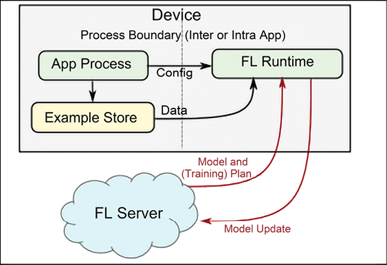
Figure 19.15: An example of federated learning architecture

TensorFlow FL APIs

The TensorFlow Federated (TTF) platform has two layers:

• Federated learning (FL), as discussed earlier, is a high-level interface that works well with tf.keras and non-tf.keras models. In the majority of situations, we will use this API for distributed training that is privacy-preserving.
• Federated core (FC), a low-level interface that is highly customizable and allows you to interact with low-level communications and with federated algorithms. You will need this API only if you intend to implement new and sophisticated distributed learning algorithms. This topic is rather advanced, and we are not going to cover it in this book. If you wish to learn more, you can find more information online (https://www.tensorflow.org/federated/federated_core).

The FL API has three key parts:

1. Models: Used to wrap existing models for enabling federating learning. This can be achieved via the tff.learning.from_keras_model(), or via the subclassing of tff.learning.Model(). For instance, you can have the following code fragment:

   keras_model = …
   keras_model.compile(...)
   keras_federated_model = tff.learning.from_compiled_keras_model(keras_model, ..)
   
2. Builders: This is the layer where the federated computation happens. There are two phases: compilation, where the learning algorithm is serialized into an abstract representation of the computation, and execution, where the represented computation is run.
3. Datasets: This is a large collection of data that can be used to simulate federated learning locally – a useful step for initial fine-tuning.

We conclude this overview by mentioning that you can find a detailed description of the APIs online and also a number of coding examples (https://www.tensorflow.org/federated/federated_learning). Start by using the Colab notebook made available by Google (https://colab.research.google.com/github/tensorflow/federated/blob/v0.10.1/docs/tutorials/federated_learning_for_image_classification.ipynb). The framework allows us to simulate the distributed training before running it in a real environment. The library in charge of FL learning is tensorflow_federated. Figure 19.16 discusses all the steps used in federated learning with multiple nodes, and it might be useful to better understand what has been discussed in this section:

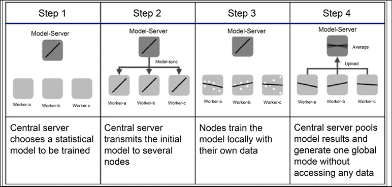
Figure 19.16: An example of federated learning with multiple nodes (source: https://upload.wikimedia.org/wikipedia/commons/e/e2/Federated_learning_process_central_case.png)

The next section will introduce TensorFlow.js, a variant of TensorFlow that can be used natively in JavaScript.

TensorFlow.js

TensorFlow.js is a JavaScript library for machine learning models that can work either in vanilla mode or via Node.js. In this section, we are going to review both of them.

Vanilla TensorFlow.js

TensorFlow.js is a JavaScript library for training and using machine learning models in a browser. It is derived from deeplearn.js, an open-source, hardware-accelerated library for doing deep learning in JavaScript, and is now a companion library to TensorFlow.

The most common use of TensorFlow.js is to make pretrained ML/DL models available on the browser. This can help in situations where it may not be feasible to send client data back to the server due to network bandwidth or security concerns. However, TensorFlow.js is a full-stack ML platform, and it is possible to build and train an ML/DL model from scratch, as well as fine-tune an existing pretrained model with new client data.

An example of a TensorFlow.js application is the TensorFlow Projector (https://projector.tensorflow.org), which allows a client to visualize their own data (as word vectors) in 3-dimensional space, using one of several dimensionality reduction algorithms provided. There are a few other examples of TensorFlow.js applications listed on the TensorFlow.js demo page (https://www.tensorflow.org/js/demos).

Similar to TensorFlow, TensorFlow.js also provides two main APIs – the Ops API, which exposes low-level tensor operations such as matrix multiplication, and the Layers API, which exposes Keras-style high-level building blocks for neural networks.

At the time of writing, TensorFlow.js runs on three different backends. The fastest (and also the most complex) is the WebGL backend, which provides access to WebGL’s low-level 3D graphics APIs and can take advantage of GPU hardware acceleration. The other popular backend is the Node.js backend, which allows the use of TensorFlow.js in server-side applications. Finally, as a fallback, there is the CPU-based implementation in plain JavaScript that will run in any browser.

In order to gain a better understanding of how to write a TensorFlow.js application, we will walk through an example of classifying MNIST digits using a CNN provided by the TensorFlow.js team (https://storage.googleapis.com/tfjs-examples/mnist/dist/index.html).

The steps here are similar to a normal supervised model development pipeline – load the data, define, train, and evaluate the model.

JavaScript works inside a browser environment, within an HTML page. The HTML file (named index.html) below represents this HTML page. Notice the two imports for TensorFlow.js (tf.min.js) and the TensorFlow.js visualization library (tfjs-vis.umd.min.js) – these provide library functions that we will use in our application. The JavaScript code for our application comes from data.js and script.js files, located in the same directory as our index.html file:

<!DOCTYPE html>
<html>
<head>
  <meta charset="utf-8">
  <meta http-equiv="X-UA-Compatible" content="IE=edge">
  <meta name="viewport" content="width=device-width, initial-scale=1.0">
  <!-- Import TensorFlow.js -->
  <script src="https://cdn.jsdelivr.net/npm/@tensorflow/[email protected]/dist/tf.min.js"></script>
  <!-- Import tfjs-vis -->
  <script src="https://cdn.jsdelivr.net/npm/@tensorflow/[email protected]/dist/tfjs-vis.umd.min.js"></script>
  <!-- Import the data file -->
  <script src="data.js" type="module"></script>
  <!-- Import the main script file -->
  <script src="script.js" type="module"></script>
</head>
<body>
</body>
</html>

For deployment, we will deploy these three files (index.html, data.js, and script.js) on a web server, but for development, we can start a web server up by calling a simple one bundled with the Python distribution. This will start up a web server on port 8000 on localhost, and the index.html file can be rendered on the browser at http://localhost:8000:

python -m http.server

The next step is to load the data. Fortunately, Google provides a JavaScript script that we have called directly from our index.html file. It downloads the images and labels from GCP storage and returns shuffled and normalized batches of image and label pairs for training and testing. We can download this to the same folder as the index.html file using the following command:

wget -cO - https://storage.googleapis.com/tfjs-tutorials/mnist_data.js > data.js

Model definition, training, and evaluation code is all specified inside the script.js file. The function to define and build the network is shown in the following code block. As you can see, it is very similar to the way you would build a sequential model with tf.keras. The only difference is the way you specify the arguments, as a dictionary of name-value pairs instead of a list of parameters. The model is a sequential model, that is, a list of layers. Finally, the model is compiled with the Adam optimizer:

function getModel() {
  const IMAGE_WIDTH = 28;
  const IMAGE_HEIGHT = 28;
  const IMAGE_CHANNELS = 1;  
  const NUM_OUTPUT_CLASSES = 10;
  
  const model = tf.sequential();
  model.add(tf.layers.conv2d({
    inputShape: [IMAGE_WIDTH, IMAGE_HEIGHT, IMAGE_CHANNELS],
    kernelSize: 5,
    filters: 8,
    strides: 1,
    activation: 'relu',
    kernelInitializer: 'varianceScaling'
  }));
  model.add(tf.layers.maxPooling2d({
    poolSize: [2, 2], strides: [2, 2]
  }));
  model.add(tf.layers.conv2d({
    kernelSize: 5,
    filters: 16,
    strides: 1,
    activation: 'relu',
    kernelInitializer: 'varianceScaling'
  }));
  model.add(tf.layers.maxPooling2d({
    poolSize: [2, 2], strides: [2, 2]
  }));
  model.add(tf.layers.flatten());
  model.add(tf.layers.dense({
    units: NUM_OUTPUT_CLASSES,
    kernelInitializer: 'varianceScaling',
    activation: 'softmax'
  }));
  const optimizer = tf.train.adam();
  model.compile({
    optimizer: optimizer,
    loss: 'categoricalCrossentropy',
    metrics: ['accuracy'],
  });
  return model;
}

The model is then trained for 10 epochs with batches from the training dataset and validated inline using batches from the test dataset. A best practice is to create a separate validation dataset from the training set. However, to keep our focus on the more important aspect of showing how to use TensorFlow.js to design an end-to-end DL pipeline, we are using the external data.js file provided by Google, which provides functions to return only a training and test batch. In our example, we will use the test dataset for validation as well as evaluation later.

This is likely to give us better accuracies compared to what we would have achieved with an unseen (during training) test set, but that is unimportant for an illustrative example such as this one:

async function train(model, data) {
  const metrics = ['loss', 'val_loss', 'acc', 'val_acc'];
  const container = {
    name: 'Model Training', tab: 'Model', styles: { height: '1000px' }
  };
  const fitCallbacks = tfvis.show.fitCallbacks(container, metrics);
  
  const BATCH_SIZE = 512;
  const TRAIN_DATA_SIZE = 5500;
  const TEST_DATA_SIZE = 1000;
  const [trainXs, trainYs] = tf.tidy(() => {
    const d = data.nextTrainBatch(TRAIN_DATA_SIZE);
    return [
      d.xs.reshape([TRAIN_DATA_SIZE, 28, 28, 1]),
      d.labels
    ];
  });
  const [testXs, testYs] = tf.tidy(() => {
    const d = data.nextTestBatch(TEST_DATA_SIZE);
    return [
      d.xs.reshape([TEST_DATA_SIZE, 28, 28, 1]),
      d.labels
    ];
  });
  return model.fit(trainXs, trainYs, {
    batchSize: BATCH_SIZE,
    validationData: [testXs, testYs],
    epochs: 10,
    shuffle: true,
    callbacks: fitCallbacks
  });
}

Once the model finishes training, we want to make predictions and evaluate the model on its predictions. The following functions will do the predictions and compute the overall accuracy for each of the classes over all the test set examples, as well as produce a confusion matrix across all the test set samples:

const classNames = [
  'Zero', 'One', 'Two', 'Three', 'Four', 
  'Five', 'Six', 'Seven', 'Eight', 'Nine'];
function doPrediction(model, data, testDataSize = 500) {
  const IMAGE_WIDTH = 28;
  const IMAGE_HEIGHT = 28;
  const testData = data.nextTestBatch(testDataSize);
  const testxs = testData.xs.reshape(
    [testDataSize, IMAGE_WIDTH, IMAGE_HEIGHT, 1]);
  const labels = testData.labels.argMax([-1]);
  const preds = model.predict(testxs).argMax([-1]);
  testxs.dispose();
  return [preds, labels];
}
async function showAccuracy(model, data) {
  const [preds, labels] = doPrediction(model, data);
  const classAccuracy = await tfvis.metrics.perClassAccuracy(
    labels, preds);
  const container = {name: 'Accuracy', tab: 'Evaluation'};
  tfvis.show.perClassAccuracy(container, classAccuracy, classNames);
  labels.dispose();
}
async function showConfusion(model, data) {
  const [preds, labels] = doPrediction(model, data);
  const confusionMatrix = await tfvis.metrics.confusionMatrix(
    labels, preds);
  const container = {name: 'Confusion Matrix', tab: 'Evaluation'};
  tfvis.render.confusionMatrix(
      container, {values: confusionMatrix}, classNames);
  labels.dispose();
}

Finally, the run() function will call all these functions in sequence to build an end-to-end ML pipeline:

import {MnistData} from './data.js';
async function run() { 
  const data = new MnistData();
  await data.load();
  await showExamples(data);
  const model = getModel();
  tfvis.show.modelSummary({name: 'Model Architecture', tab: 'Model'}, model);
  await train(model, data);
  await showAccuracy(model, data);
  await showConfusion(model, data);
}
document.addEventListener('DOMContentLoaded', run);

Refreshing the browser location, http://localhost:8000/index.html, will invoke the run() method above. Figure 19.17 shows the model architecture and the plots of the progress of the training.

On the left are the loss and accuracy values on the validation dataset observed at the end of each batch, and on the right are the same loss and accuracy values observed on the training dataset (blue) and validation dataset (red) at the end of each epoch:

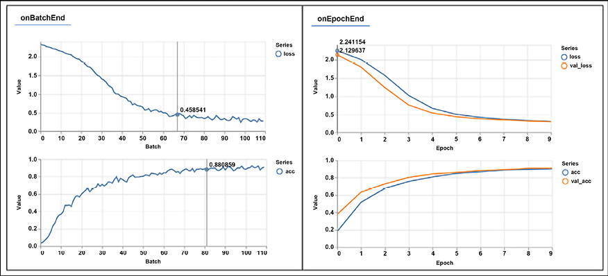
Figure 19.17: Model loss and accuracy as it is being trained

In addition, the following figure shows the accuracies across different classes for predictions from our trained model on the test dataset, as well as the confusion matrix of predicted versus actual classes for test dataset samples:

Figure 19.18: Confusion metrics and accuracy for each class as obtained by the trained model

Readers might enjoy seeing this live example from the TensorFlow team training a TFJS model on the MNIST dataset: https://storage.googleapis.com/tfjs-examples/mnist/dist/index.html.

We have seen how to use TensorFlow.js within the browser. The next section will explain how to convert a model from Keras into TensorFlow.js.

Converting models

Sometimes it is convenient to convert a model that has already been created with tf.keras. This is very easy and can be done offline with the following command, which takes a Keras model from /tmp/model.h5 and outputs a JavaScript model into /tmp/tfjs_model:

tensorflowjs_converter --input_format=keras /tmp/model.h5 /tmp/tfjs_model

To be able to use this command, you will need a Python environment with TensorFlow JS installed using:

pip install tensorflowjs

This will install the above converter. The next section will explain how to use pretrained models in TensorFlow.js.

Pretrained models

TensorFlow.js comes with a significant number of pretrained models for deep learning with image, video, and text. The models are hosted on npm, so it’s very simple to use them if you are familiar with Node.js development.

Table 19.1 summarizes some of the pretrained models available as of August 2022 (source: https://github.com/tensorflow/tfjs-models):

Table 19.1: A list of some of the pretrained models on TensorFlow.js

Each pretrained model can be directly used from HTML. For instance, this is an example with the KNN classifier:

<html>
  <head>
    <!-- Load TensorFlow.js -->
    <script src="https://cdn.jsdelivr.net/npm/@tensorflow/tfjs"></script>
    <!-- Load MobileNet -->
    <script src="https://cdn.jsdelivr.net/npm/@tensorflow-models/mobilenet"></script>
    <!-- Load KNN Classifier -->
    <script src="https://cdn.jsdelivr.net/npm/@tensorflow-models/knn-classifier"></script>
  </head>

The next section will explain how to use pretrained models in Node.js.

Node.js

In this section, we will give an overview of how to use TensorFlow with Node.js. Let’s start.

The CPU package is imported with the following line of code, which will work for all macOS, Linux, and Windows platforms:

import * as tf from '@tensorflow/tfjs-node'

The GPU package is imported with the following line of code (as of November 2019, this will work only on a GPU in a CUDA environment):

import * as tf from '@tensorflow/tfjs-node-gpu'

An example of Node.js code for defining and compiling a simple dense model is reported below. The code is self-explanatory:

const model = tf.sequential();
model.add(tf.layers.dense({ units: 1, inputShape: [400] }));
model.compile({
  loss: 'meanSquaredError',
  optimizer: 'sgd',
  metrics: ['MAE']
});

Training can then start with the typical Node.js asynchronous invocation:

const xs = tf.randomUniform([10000, 400]);
const ys = tf.randomUniform([10000, 1]);
const valXs = tf.randomUniform([1000, 400]);
const valYs = tf.randomUniform([1000, 1]);
async function train() {
  await model.fit(xs, ys, {
    epochs: 100,
    validationData: [valXs, valYs],
  });
}
train();

In this section, we have discussed how to use TensorFlow.js with both vanilla JavaScript and Node.js using sample applications for both the browser and backend computation.

Summary

In this chapter, we have discussed different components of the TensorFlow ecosystem. We started with TensorFlow Hub, the place where many pretrained models are available. Next, we talked about the TensorFlow Datasets and learned how to build a data pipeline using TFDS. We learned how to use TensorFlow Lite for mobile devices and IoT and deployed real applications on Android devices. Then, we also talked about federated learning for distributed learning across thousands (millions) of mobile devices, taking into account privacy concerns. The last section of the chapter was devoted to TensorFlow.js for using TensorFlow with vanilla JavaScript or with Node.js.

The next chapter is about advanced CNNs, where you will learn some advanced CNN architectures and their applications.

References

1. Quantization-aware training: https://github.com/tensorflow/tensorflow/tree/r1.13/tensorflow/contrib/quantize
2. Jacob, B., Kligys, S., Chen, B., Zhu, M., Tang, M., Howard, A., Adam, H., and Kalenichenko, D. (Submitted on 15 Dec 2017). Quantization and Training of Neural Networks for Efficient Integer-Arithmetic-Only Inference. https://arxiv.org/abs/1712.05877
3. Sandler, M., Howard, A., Zhu, M., Zhmoginov, A., Chen, L-C. (Submitted on 13 Jan 2018 (v1), last revised 21 Mar 2019 (v4)). MobileNetV2: Inverted Residuals and Linear Bottlenecks. https://arxiv.org/abs/1806.08342
4. Tan, M., Chen, B., Pang, R., Vasudevan, V., Sandler, M., Howard, A., and Le, Q. V. MnasNet: Platform-Aware Neural Architecture Search for Mobile. https://arxiv.org/abs/1807.11626
5. Chen, L-C., Papandreou, G., Kokkinos, I., Murphy, K., and Yuille, A. L. (May 2017). DeepLab: Semantic Image Segmentation with Deep Convolutional Nets, Atrous Convolution, and Fully Connected CRFs. https://arxiv.org/pdf/1606.00915.pdf
6. Devlin, J., Chang, M-W., Lee, K., and Toutanova, K. (Submitted on 11 Oct 2018 (v1), last revised 24 May 2019 v2). BERT: Pre-training of Deep Bidirectional Transformers for Language Understanding. https://arxiv.org/abs/1810.04805
7. Anonymous authors, Paper under double-blind review. (modified: 25 Sep 2019). MOBILEBERT: TASK-AGNOSTIC COMPRESSION OF BERT BY PROGRESSIVE KNOWLEDGE TRANSFER. ICLR 2020 Conference Blind Submission Readers: Everyone. https://openreview.net/pdf?id=SJxjVaNKwB
8. McMahan, H. B., Moore, E., Ramage, D., Hampson, and S., Arcas, B. A. y. (Submitted on 17 Feb 2016 (v1), last revised 28 Feb 2017 (this version, v3)). Communication-Efficient Learning of Deep Networks from Decentralized Data. https://arxiv.org/abs/1602.05629
9. Konečný, J., McMahan, H. B., Yu, F. X., Richtárik, P., Suresh, A. T., and Bacon, D. (Submitted on 18 Oct 2016 (v1), last revised 30 Oct 2017 (this version, v2)). Federated Learning: Strategies for Improving Communication Efficiency. https://arxiv.org/abs/1610.05492
10. Bonawitz, K. et al. (22 March 2019). TOWARDS FEDERATED LEARNING AT SCALE: SYSTEM DESIGN. https://arxiv.org/pdf/1902.01046.pdf

Join our book’s Discord space

Join our Discord community to meet like-minded people and learn alongside more than 2000 members at: https://packt.link/keras