2
Regression and Classification
Regression and classification are two fundamental tasks ubiquitously present in almost all machine learning applications. They find application in varied fields ranging from engineering, physical science, biology, and the financial market, to the social sciences. They are the fundamental tools in the hands of statisticians and data scientists. In this chapter, we will cover the following topics:
- Regression
- Classification
- Difference between classification and regression
- Linear regression
- Different types of linear regression
- Classification using the TensorFlow Keras API
- Applying linear regression to estimate the price of a house
- Applying logistic regression to identify handwritten digits
All the code files for this chapter can be found at https://packt.link/dltfchp2
Let us first start with understanding what regression really is.
What is regression?
Regression is normally the first algorithm that people in machine learning work with. It allows us to make predictions from data by learning about the relationship between a given set of dependent and independent variables. It has its use in almost every field; anywhere that has an interest in drawing relationships between two or more things will find a use for regression.
Consider the case of house price estimation. There are many factors that can have an impact on the house price: the number of rooms, the floor area, the locality, the availability of amenities, the parking space, and so on. Regression analysis can help us in finding the mathematical relationship between these factors and the house price.
Let us imagine a simpler world where only the area of the house determines its price. Using regression, we could determine the relationship between the area of the house (independent variable: these are the variables that do not depend upon any other variables) and its price (dependent variable: these variables depend upon one or more independent variables). Later, we could use this relationship to predict the price of any house, given its area. To learn more about dependent and independent variables and how to identify them, you can refer to this post: https://medium.com/deeplearning-concepts-and-implementation/independent-and-dependent-variables-in-machine-learning-210b82f891db. In machine learning, the independent variables are normally input into the model and the dependent variables are output from our model.
Depending upon the number of independent variables, the number of dependent variables, and the relationship type, we have many different types of regression. There are two important components of regression: the relationship between independent and dependent variables, and the strength of impact of different independent variables on dependent variables. In the following section, we will learn in detail about the widely used linear regression technique.
Prediction using linear regression
Linear regression is one of the most widely known modeling techniques. Existing for more than 200 years, it has been explored from almost all possible angles. Linear regression assumes a linear relationship between the input variable (X) and the output variable (Y). The basic idea of linear regression is building a model, using training data that can predict the output given the input, such that the predicted output ![]() is as near the observed training output Y for the input X. It involves finding a linear equation for the predicted value
is as near the observed training output Y for the input X. It involves finding a linear equation for the predicted value ![]() of the form:
of the form:
![]()
where ![]() are the n input variables, and
are the n input variables, and  are the linear coefficients, with b as the bias term. We can also expand the preceding equation to:

The bias term allows our regression model to provide an output even in the absence of any input; it provides us with an option to shift our data for a better fit. The error between the observed values (Y) and predicted values (![]() ) for an input sample i is:
) for an input sample i is:

The goal is to find the best estimates for the coefficients W and bias b, such that the error between the observed values Y and the predicted values ![]() is minimized. Let’s go through some examples to better understand this.
is minimized. Let’s go through some examples to better understand this.
Simple linear regression
If we consider only one independent variable and one dependent variable, what we get is a simple linear regression. Consider the case of house price prediction, defined in the preceding section; the area of the house (A) is the independent variable, and the price (Y) of the house is the dependent variable. We want to find a linear relationship between predicted price ![]() and A, of the form:
and A, of the form:
![]()
where b is the bias term. Thus, we need to determine W and b, such that the error between the price Y and the predicted price ![]() is minimized. The standard method used to estimate W and b is called the method of least squares, that is, we try to minimize the sum of the square of errors (S). For the preceding case, the expression becomes:
is minimized. The standard method used to estimate W and b is called the method of least squares, that is, we try to minimize the sum of the square of errors (S). For the preceding case, the expression becomes:

We want to estimate the regression coefficients, W and b, such that S is minimized. We use the fact that the derivative of a function is 0 at its minima to get these two equations:
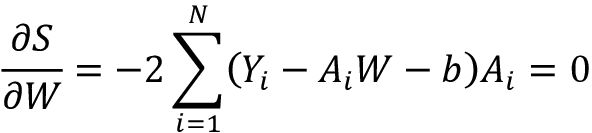
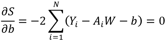
These two equations can be solved to find the two unknowns. To do so, we first expand the summation in the second equation:

Take a look at the last term on the left-hand side; it just sums up a constant N time. Thus, we can rewrite it as:

Reordering the terms, we get:

The two terms on the right-hand side can be replaced by ![]() , the average price (output), and
, the average price (output), and ![]() , the average area (input), respectively, and thus we get:
, the average area (input), respectively, and thus we get:
![]()
In a similar fashion, we expand the partial differential equation of S with respect to weight W:

Substitute the expression for the bias term b:

Reordering the equation:

Playing around with the mean definition, we can get from this the value of weight W as:

where ![]() and
and ![]() are the average price and area, respectively. Let us try this on some simple sample data:
are the average price and area, respectively. Let us try this on some simple sample data:
- We import the necessary modules. It is a simple example, so we’ll be using only NumPy, pandas, and Matplotlib:
import tensorflow as tf import numpy as np import matplotlib.pyplot as plt import pandas as pd - Next, we generate random data with a linear relationship. To make it more realistic, we also add a random noise element. You can see the two variables (the cause,
area, and the effect,price) follow a positive linear dependence:#Generate a random data np.random.seed(0) area = 2.5 * np.random.randn(100) + 25 price = 25 * area + 5 + np.random.randint(20,50, size = len(area)) data = np.array([area, price]) data = pd.DataFrame(data = data.T, columns=['area','price']) plt.scatter(data['area'], data['price']) plt.show()

Figure 2.1: Scatter plot between the area of the house and its price
- Now, we calculate the two regression coefficients using the equations we defined. You can see the result is very much near the linear relationship we have simulated:
W = sum(price*(area-np.mean(area))) / sum((area-np.mean(area))**2) b = np.mean(price) - W*np.mean(area) print("The regression coefficients are", W,b)----------------------------------------------- The regression coefficients are 24.815544052284988 43.4989785533412 - Let us now try predicting the new prices using the obtained weight and bias values:
y_pred = W * area + b - Next, we plot the predicted prices along with the actual price. You can see that predicted prices follow a linear relationship with the area:
plt.plot(area, y_pred, color='red',label="Predicted Price") plt.scatter(data['area'], data['price'], label="Training Data") plt.xlabel("Area") plt.ylabel("Price") plt.legend()
Figure 2.2: Predicted values vs the actual price
From Figure 2.2, we can see that the predicted values follow the same trend as the actual house prices.
Multiple linear regression
The preceding example was simple, but that is rarely the case. In most problems, the dependent variables depend upon multiple independent variables. Multiple linear regression finds a linear relationship between the many independent input variables (X) and the dependent output variable (Y), such that they satisfy the predicted Y value of the form:
![]()
where  are the n independent input variables, and are the linear coefficients, with b as the bias term.
As before, the linear coefficients Ws are estimated using the method of least squares, that is, minimizing the sum of squared differences between predicted values (![]() ) and observed values (Y). Thus, we try to minimize the loss function (also called squared error, and if we divide by n, it is the mean squared error):
) and observed values (Y). Thus, we try to minimize the loss function (also called squared error, and if we divide by n, it is the mean squared error):

where the sum is over all the training samples.
As you might have guessed, now, instead of two, we will have n+1 equations, which we will need to simultaneously solve. An easier alternative will be to use the TensorFlow Keras API. We will learn shortly how to use the TensorFlow Keras API to perform the task of regression.
Multivariate linear regression
There can be cases where the independent variables affect more than one dependent variable. For example, consider the case where we want to predict a rocket’s speed and its carbon dioxide emission – these two will now be our dependent variables, and both will be affected by the sensors reading the fuel amount, engine type, rocket body, and so on. This is a case of multivariate linear regression. Mathematically, a multivariate regression model can be represented as:

where ![]() and
and  . The term
 ![]() represents the jth predicted output value corresponding to the ith input sample, w represents the regression coefficients, and xik is the kth feature of the ith input sample. The number of equations needed to solve in this case will now be n x m. While we can solve these equations using matrices, the process will be computationally expensive as it will involve calculating the inverse and determinants. An easier way would be to use the gradient descent with the sum of least square error as the loss function and to use one of the many optimizers that the TensorFlow API includes.
represents the jth predicted output value corresponding to the ith input sample, w represents the regression coefficients, and xik is the kth feature of the ith input sample. The number of equations needed to solve in this case will now be n x m. While we can solve these equations using matrices, the process will be computationally expensive as it will involve calculating the inverse and determinants. An easier way would be to use the gradient descent with the sum of least square error as the loss function and to use one of the many optimizers that the TensorFlow API includes.
In the next section, we will delve deeper into the TensorFlow Keras API, a versatile higher-level API to develop your model with ease.
Neural networks for linear regression
In the preceding sections, we used mathematical expressions for calculating the coefficients of a linear regression equation. In this section, we will see how we can use the neural networks to perform the task of regression and build a neural network model using the TensorFlow Keras API.
Before performing regression using neural networks, let us first review what a neural network is. Simply speaking, a neural network is a network of many artificial neurons. From Chapter 1, Neural Network Foundations with TF, we know that the simplest neural network, the (simple) perceptron, can be mathematically represented as:

where f is the activation function. Consider, if we have f as a linear function, then the above expression is similar to the expression of linear regression that we learned in the previous section. In other words, we can say that a neural network, which is also called a function approximator, is a generalized regressor. Let us try to build a neural network simple regressor next using the TensorFlow Keras API.
Simple linear regression using TensorFlow Keras
In the first chapter, we learned about how to build a model in TensorFlow Keras. Here, we will use the same Sequential API to build a single-layered perceptron (fully connected neural network) using the Dense class. We will continue with the same problem, that is, predicting the price of a house given its area:
- We start with importing the packages we will need. Notice the addition of the
Kerasmodule and theDenselayer in importing packages:import tensorflow as tf import numpy as np import matplotlib.pyplot as plt import pandas as pd import tensorflow.keras as K from tensorflow.keras.layers import Dense - Next, we generate the data, as in the previous case:
#Generate a random data np.random.seed(0) area = 2.5 * np.random.randn(100) + 25 price = 25 * area + 5 + np.random.randint(20,50, size = len(area)) data = np.array([area, price]) data = pd.DataFrame(data = data.T, columns=['area','price']) plt.scatter(data['area'], data['price']) plt.show() - The input to neural networks should be normalized; this is because input gets multiplied with weights, and if we have very large numbers, the result of multiplication will be large, and soon our metrics may cross infinity (the largest number your computer can handle):
data = (data - data.min()) / (data.max() - data.min()) #Normalize - Let us now build the model; since it is a simple linear regressor, we use a
Denselayer with only one unit:model = K.Sequential([ Dense(1, input_shape = [1,], activation=None) ]) model.summary()Model: "sequential" ____________________________________________________________ Layer (type) Output Shape Param # ============================================================ dense (Dense) (None, 1) 2 ============================================================ Total params: 2 Trainable params: 2 Non-trainable params: 0 ____________________________________________________________ - To train a model, we will need to define the loss function and optimizer. The loss function defines the quantity that our model tries to minimize, and the optimizer decides the minimization algorithm we are using. Additionally, we can also define metrics, which is the quantity we want to log as the model is trained. We define the loss function,
optimizer(see Chapter 1, Neural Network Foundations with TF), and metrics using thecompilefunction:model.compile(loss='mean_squared_error', optimizer='sgd') - Now that model is defined, we just need to train it using the
fitfunction. Observe that we are using abatch_sizeof 32 and splitting the data into training and validation datasets using thevalidation_spiltargument of thefitfunction:model.fit(x=data['area'],y=data['price'], epochs=100, batch_size=32, verbose=1, validation_split=0.2)model.fit(x=data['area'],y=data['price'], epochs=100, batch_size=32, verbose=1, validation_split=0.2) Epoch 1/100 3/3 [==============================] - 0s 78ms/step - loss: 1.2643 - val_loss: 1.4828 Epoch 2/100 3/3 [==============================] - 0s 13ms/step - loss: 1.0987 - val_loss: 1.3029 Epoch 3/100 3/3 [==============================] - 0s 13ms/step - loss: 0.9576 - val_loss: 1.1494 Epoch 4/100 3/3 [==============================] - 0s 16ms/step - loss: 0.8376 - val_loss: 1.0156 Epoch 5/100 3/3 [==============================] - 0s 15ms/step - loss: 0.7339 - val_loss: 0.8971 Epoch 6/100 3/3 [==============================] - 0s 16ms/step - loss: 0.6444 - val_loss: 0.7989 Epoch 7/100 3/3 [==============================] - 0s 14ms/step - loss: 0.5689 - val_loss: 0.7082 . . . Epoch 96/100 3/3 [==============================] - 0s 22ms/step - loss: 0.0827 - val_loss: 0.0755 Epoch 97/100 3/3 [==============================] - 0s 17ms/step - loss: 0.0824 - val_loss: 0.0750 Epoch 98/100 3/3 [==============================] - 0s 14ms/step - loss: 0.0821 - val_loss: 0.0747 Epoch 99/100 3/3 [==============================] - 0s 21ms/step - loss: 0.0818 - val_loss: 0.0740 Epoch 100/100 3/3 [==============================] - 0s 15ms/step - loss: 0.0815 - val_loss: 0.0740 <keras.callbacks.History at 0x7f7228d6a790> - Well, you have successfully trained a neural network to perform the task of linear regression. The mean squared error after training for 100 epochs is 0.0815 on training data and 0.074 on validation data. We can get the predicted value for a given input using the
predictfunction:y_pred = model.predict(data['area']) - Next, we plot a graph of the predicted and the actual data:
plt.plot(data['area'], y_pred, color='red',label="Predicted Price") plt.scatter(data['area'], data['price'], label="Training Data") plt.xlabel("Area") plt.ylabel("Price") plt.legend() - Figure 2.3 shows the plot between the predicted data and the actual data. You can see that, just like the linear regressor, we have got a nice linear fit:

Figure 2.3: Predicted price vs actual price
- In case you are interested in knowing the coefficients
Wandb, we can do it by printing the weights of the model usingmodel.weights:[<tf.Variable 'dense/kernel:0' shape=(1, 1) dtype=float32, numpy=array([[-0.33806288]], dtype=float32)>, <tf.Variable 'dense/bias:0' shape=(1,) dtype=float32, numpy=array([0.68142694], dtype=float32)>]
We can see from the result above that our coefficients are W= 0.69 and bias b= 0.127. Thus, using linear regression, we can find a linear relationship between the house price and its area. In the next section, we explore multiple and multivariate linear regression using the TensorFlow Keras API.
Multiple and multivariate linear regression using the TensorFlow Keras API
The example in the previous section had only one independent variable, the area of the house, and one dependent variable, the price of the house. However, problems in real life are not that simple; we may have more than one independent variable, and we may need to predict more than one dependent variable. As you must have realized from the discussion on multiple and multivariate regression, they involve solving multiple equations. We can make our tasks easier by using the Keras API for both tasks.
Additionally, we can have more than one neural network layer, that is, we can build a deep neural network. A deep neural network is like applying multiple function approximators:

with ![]() being the function at layer L. From the expression above, we can see that if f was a linear function, adding multiple layers of a neural network was not useful; however, using a non-linear activation function (see Chapter 1, Neural Network Foundations with TF, for more details) allows us to apply neural networks to the regression problems where dependent and independent variables are related in some non-linear fashion. In this section, we will use a deep neural network, built using TensorFlow Keras, to predict the fuel efficiency of a car, given its number of cylinders, displacement, acceleration, and so on. The data we use is available from the UCI ML repository (Blake, C., & Merz, C. (1998), the UCI repository of machine learning databases (http://www.ics.uci.edu/~mlearn/MLRepository.html):
being the function at layer L. From the expression above, we can see that if f was a linear function, adding multiple layers of a neural network was not useful; however, using a non-linear activation function (see Chapter 1, Neural Network Foundations with TF, for more details) allows us to apply neural networks to the regression problems where dependent and independent variables are related in some non-linear fashion. In this section, we will use a deep neural network, built using TensorFlow Keras, to predict the fuel efficiency of a car, given its number of cylinders, displacement, acceleration, and so on. The data we use is available from the UCI ML repository (Blake, C., & Merz, C. (1998), the UCI repository of machine learning databases (http://www.ics.uci.edu/~mlearn/MLRepository.html):
- We start by importing the modules that we will need. In the previous example, we normalized our data using the DataFrame operations. In this example, we will make use of the Keras
Normalizationlayer. TheNormalizationlayer shifts the data to a zero mean and one standard deviation. Also, since we have more than one independent variable, we will use Seaborn to visualize the relationship between different variables:import tensorflow as tf import numpy as np import matplotlib.pyplot as plt import pandas as pd import tensorflow.keras as K from tensorflow.keras.layers import Dense, Normalization import seaborn as sns - Let us first download the data from the UCI ML repo.
url = 'https://archive.ics.uci.edu/ml/machine-learning-databases/auto-mpg/auto-mpg.data' column_names = ['mpg', 'cylinders', 'displacement', 'horsepower', 'weight', 'acceleration', 'model_year', 'origin'] data = pd.read_csv(url, names=column_names, na_values='?', comment=' ', sep=' ', skipinitialspace=True) - The data consists of eight features: mpg, cylinders, displacement, horsepower, weight, acceleration, model year, and origin. Though the origin of the vehicle can also affect the fuel efficiency “mpg” (miles per gallon), we use only seven features to predict the mpg value. Also, we drop any rows with NaN values:
data = data.drop('origin', 1) print(data.isna().sum()) data = data.dropna() - We divide the dataset into training and test datasets. Here, we are keeping 80% of the 392 datapoints as training data and 20% as test dataset:
train_dataset = data.sample(frac=0.8, random_state=0) test_dataset = data.drop(train_dataset.index) - Next, we use Seaborn’s
pairplotto visualize the relationship between the different variables:sns.pairplot(train_dataset[['mpg', 'cylinders', 'displacement','horsepower', 'weight', 'acceleration', 'model_year']], diag_kind='kde') - We can see that mpg (fuel efficiency) has dependencies on all the other variables, and the dependency relationship is non-linear, as none of the curves are linear:

Figure 2.4: Relationship among different variables of auto-mpg data
- For convenience, we also separate the variables into input variables and the label that we want to predict:
train_features = train_dataset.copy() test_features = test_dataset.copy() train_labels = train_features.pop('mpg') test_labels = test_features.pop('mpg') - Now, we use the Normalization layer of Keras to normalize our data. Note that while we normalized our inputs to a value with mean 0 and standard deviation 1, the output prediction
'mpg'remains as it is:#Normalize data_normalizer = Normalization(axis=1) data_normalizer.adapt(np.array(train_features)) - We build our model. The model has two hidden layers, with 64 and 32 neurons, respectively. For the hidden layers, we have used Rectified Linear Unit (ReLU) as our activation function; this should help in approximating the non-linear relation between fuel efficiency and the rest of the variables:
model = K.Sequential([ data_normalizer, Dense(64, activation='relu'), Dense(32, activation='relu'), Dense(1, activation=None) ]) model.summary() - Earlier, we used stochastic gradient as the optimizer; this time, we try the Adam optimizer (see Chapter 1, Neural Network Foundations with TF, for more details). The loss function for the regression we chose is the mean squared error again:
model.compile(optimizer='adam', loss='mean_squared_error') - Next, we train the model for 100 epochs:
history = model.fit(x=train_features,y=train_labels, epochs=100, verbose=1, validation_split=0.2) - Cool, now that the model is trained, we can check if our model is overfitted, underfitted, or properly fitted by plotting the loss curve. Both validation loss and training loss are near each other as we increase the training epochs; this suggests that our model is properly trained:
plt.plot(history.history['loss'], label='loss')
plt.plot(history.history['val_loss'], label='val_loss')
plt.xlabel('Epoch')
plt.ylabel('Error [MPG]')
plt.legend()
plt.grid(True)

Figure 2.5: Model error
- Let us finally compare the predicted fuel efficiency and the true fuel efficiency on the test dataset. Remember that the model has not seen a test dataset ever, thus this prediction is from the model’s ability to generalize the relationship between inputs and fuel efficiency. If the model has learned the relationship well, the two should form a linear relationship:
y_pred = model.predict(test_features).flatten()
a = plt.axes(aspect='equal')
plt.scatter(test_labels, y_pred)
plt.xlabel('True Values [MPG]')
plt.ylabel('Predictions [MPG]')
lims = [0, 50]
plt.xlim(lims)
plt.ylim(lims)
plt.plot(lims, lims)

Figure 2.6: Plot between predicted fuel efficiency and actual values
- Additionally, we can also plot the error between the predicted and true fuel efficiency:
error = y_pred - test_labels
plt.hist(error, bins=30)
plt.xlabel('Prediction Error [MPG]')
plt.ylabel('Count')
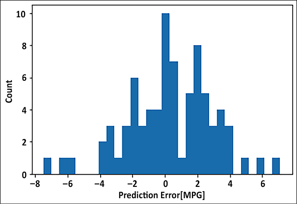
Figure 2.7: Prediction error
In case we want to make more than one prediction, that is, dealing with a multivariate regression problem, the only change would be that instead of one unit in the last dense layer, we will have as many units as the number of variables to be predicted. Consider, for example, we want to build a model which takes into account a student’s SAT score, attendance, and some family parameters, and wants to predict the GPA score for all four undergraduate years; then we will have the output layer with four units. Now that you are familiar with regression, let us move toward the classification tasks.
Classification tasks and decision boundaries
Till now, the focus of the chapter was on regression. In this section, we will talk about another important task: the task of classification. Let us first understand the difference between regression (also sometimes referred to as prediction) and classification:
- In classification, the data is grouped into classes/categories, while in regression, the aim is to get a continuous numerical value for given data. For example, identifying the number of handwritten digits is a classification task; all handwritten digits will belong to one of the ten numbers lying between 0-9. The task of predicting the price of the house depending upon different input variables is a regression task.
- In a classification task, the model finds the decision boundaries separating one class from another. In the regression task, the model approximates a function that fits the input-output relationship.
- Classification is a subset of regression; here, we are predicting classes. Regression is much more general.
Figure 2.8 shows how classification and regression tasks differ. In classification, we need to find a line (or a plane or hyperplane in multidimensional space) separating the classes. In regression, the aim is to find a line (or plane or hyperplane) that fits the given input points:
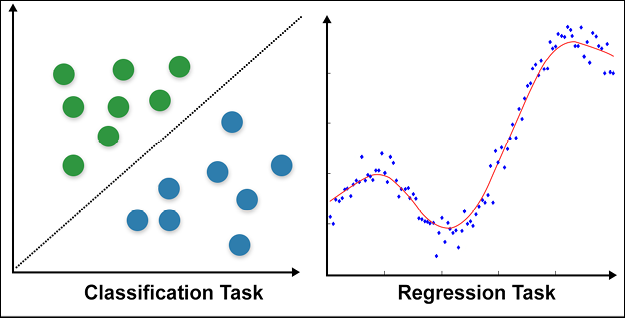
Figure 2.8: Classification vs regression
In the following section, we will explain logistic regression, which is a very common and useful classification technique.
Logistic regression
Logistic regression is used to determine the probability of an event. Conventionally, the event is represented as a categorical dependent variable. The probability of the event is expressed using the sigmoid (or “logit”) function:

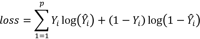
The goal now is to estimate weights and bias term b. In logistic regression, the coefficients are estimated using either the maximum likelihood estimator or stochastic gradient descent. If p is the total number of input data points, the loss is conventionally defined as a cross-entropy term given by:
Logistic regression is used in classification problems. For example, when looking at medical data, we can use logistic regression to classify whether a person has cancer or not. If the output categorical variable has two or more levels, we can use multinomial logistic regression. Another common technique used for two or more output variables is one versus all.
For multiclass logistic regression, the cross-entropy loss function is modified as:
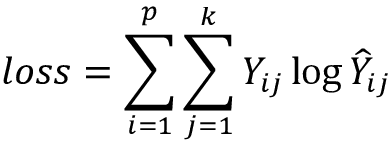
where K is the total number of classes. You can read more about logistic regression at https://en.wikipedia.org/wiki/Logistic_regression.
Now that you have some idea about logistic regression, let us see how we can apply it to any dataset.
Logistic regression on the MNIST dataset
Next, we will use TensorFlow Keras to classify handwritten digits using logistic regression. We will be using the MNIST (Modified National Institute of Standards and Technology) dataset. For those working in the field of deep learning, MNIST is not new, it is like the ABC of machine learning. It contains images of handwritten digits and a label for each image, indicating which digit it is. The label contains a value lying between 0-9 depending on the handwritten digit. Thus, it is a multiclass classification.
To implement the logistic regression, we will make a model with only one dense layer. Each class will be represented by a unit in the output, so since we have 10 classes, the number of units in the output would be 10. The probability function used in the logistic regression is similar to the sigmoid activation function; therefore, we use sigmoid activation.
Let us build our model:
- The first step is, as always, importing the modules needed. Notice that here we are using another useful layer from the Keras API, the
Flattenlayer. TheFlattenlayer helps us to resize the 28 x 28 two-dimensional input images of the MNIST dataset into a 784 flattened array:import tensorflow as tf import numpy as np import matplotlib.pyplot as plt import pandas as pd import tensorflow.keras as K from tensorflow.keras.layers import Dense, Flatten - We take the input data of MNIST from the
tensorflow.kerasdataset:((train_data, train_labels),(test_data, test_labels)) = tf.keras.datasets.mnist.load_data() - Next, we preprocess the data. We normalize the images; the MNIST dataset images are black and white images with the intensity value of each pixel lying between 0-255. We divide it by 255, so that now the values lie between 0-1:
train_data = train_data/np.float32(255) train_labels = train_labels.astype(np.int32) test_data = test_data/np.float32(255) test_labels = test_labels.astype(np.int32) - Now, we define a very simple model; it has only one
Denselayer with10units, and it takes an input of size 784. You can see from the output of the model summary that only theDenselayer has trainable parameters:model = K.Sequential([ Flatten(input_shape=(28, 28)), Dense(10, activation='sigmoid') ]) model.summary()Model: "sequential" ____________________________________________________________ Layer (type) Output Shape Param # ============================================================ flatten (Flatten) (None, 784) 0 dense (Dense) (None, 10) 7850 ============================================================ Total params: 7,850 Trainable params: 7,850 Non-trainable params: 0 ____________________________________________________________ - Since the test labels are integral values, we will use
SparseCategoricalCrossentropyloss withlogitsset toTrue. The optimizer selected is Adam. Additionally, we also define accuracy as metrics to be logged as the model is trained. We train our model for 50 epochs, with a train-validation split of 80:20:model.compile(optimizer='adam', loss=tf.keras.losses.SparseCategoricalCrossentropy(from_logits=True), metrics=['accuracy']) history = model.fit(x=train_data,y=train_labels, epochs=50, verbose=1, validation_split=0.2) - Let us see how our simple model has fared by plotting the loss plot. You can see that since the validation loss and training loss are diverging, as the training loss is decreasing, the validation loss increases, thus the model is overfitting. You can improve the model performance by adding hidden layers:
plt.plot(history.history['loss'], label='loss')
plt.plot(history.history['val_loss'], label='val_loss')
plt.xlabel('Epoch')
plt.ylabel('Loss')
plt.legend()
plt.grid(True)

Figure 2.9: Loss plot
- To better understand the result, we build two utility functions; these functions help us in visualizing the handwritten digits and the probability of the 10 units in the output:
def plot_image(i, predictions_array, true_label, img): true_label, img = true_label[i], img[i] plt.grid(False) plt.xticks([]) plt.yticks([]) plt.imshow(img, cmap=plt.cm.binary) predicted_label = np.argmax(predictions_array) if predicted_label == true_label: color ='blue' else: color ='red' plt.xlabel("Pred {} Conf: {:2.0f}% True ({})".format(predicted_label, 100*np.max(predictions_array), true_label), color=color) def plot_value_array(i, predictions_array, true_label): true_label = true_label[i] plt.grid(False) plt.xticks(range(10)) plt.yticks([]) thisplot = plt.bar(range(10), predictions_array, color"#777777") plt.ylim([0, 1]) predicted_label = np.argmax(predictions_array) thisplot[predicted_label].set_color('red') thisplot[true_label].set_color('blue') - Using these utility functions, we plot the predictions:
predictions = model.predict(test_data) i = 56 plt.figure(figsize=(10,5)) plt.subplot(1,2,1) plot_image(i, predictions[i], test_labels, test_data) plt.subplot(1,2,2) plot_value_array(i, predictions[i], test_labels) plt.show() - The plot on the left is the image of the handwritten digit, with the predicted label, the confidence in the prediction, and the true label. The image on the right shows the probability (logistic) output of the 10 units; we can see that the unit which represents the number 4 has the highest probability:
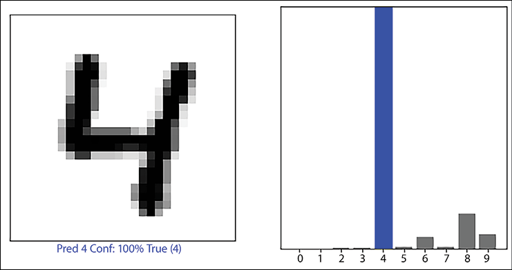
Figure 2.10: Predicted digit and confidence value of the prediction
- In this code, to stay true to logistic regression, we used a sigmoid activation function and only one
Denselayer. For better performance, adding dense layers and using softmax as the final activation function will be helpful. For example, the following model gives 97% accuracy on the validation dataset:better_model = K.Sequential([ Flatten(input_shape=(28, 28)), Dense(128, activation='relu'), Dense(10, activation='softmax') ]) better_model.summary()
You can experiment by adding more layers, or by changing the number of neurons in each layer, and even changing the optimizer. This will give you a better understanding of how these parameters influence the model performance.
Summary
This chapter dealt with different types of regression algorithms. We started with linear regression and used it to predict house prices for a simple one-input variable case. We built simple and multiple linear regression models using the TensorFlow Keras API. The chapter then moved toward logistic regression, which is a very important and useful technique for classifying tasks. The chapter explained the TensorFlow Keras API and used it to implement both linear and logistic regression for some classical datasets. The next chapter will introduce you to convolutional neural networks, the most commercially successful neural network models for image data.
References
Here are some good resources if you are interested in knowing more about the concepts we’ve covered in this chapter:
- TensorFlow website: https://www.tensorflow.org/
- Exploring bivariate numerical data: https://www.khanacademy.org/math/statistics-probability/describing-relationships-quantitative-data
- Murphy, K. P. (2022). Probabilistic Machine Learning: An introduction, MIT Press.
- Blake, C., & Merz, C. (1998). UCI repository of machine learning databases: http://www.ics.uci.edu/~mlearn/MLRepository.html
Join our book’s Discord space
Join our Discord community to meet like-minded people and learn alongside more than 2000 members at: https://packt.link/keras