4

Word Embeddings

In the previous chapter, we talked about convolutional networks, which have been very successful against image data. Over the next few chapters, we will switch tracks to focus on strategies and networks to handle text data.

In this chapter, we will first look at the idea behind word embeddings, and then cover the two earliest implementations – Word2Vec and GloVe. We will learn how to build word embeddings from scratch using the popular library Gensim on our own corpus and navigate the embedding space we create.

We will also learn how to use pretrained third-party embeddings as a starting point for our own NLP tasks, such as spam detection, that is, learning to automatically detect unsolicited and unwanted emails. We will then learn about various ways to leverage the idea of word embeddings for unrelated tasks, such as constructing an embedded space for making item recommendations.

We will then look at extensions to these foundational word embedding techniques that have occurred in the last decade since Word2Vec – adding syntactic similarity with fastText, adding the effect of context using neural networks such as ELMo and Google Universal Sentence Encoder, sentence encodings such as InferSent and skip-thoughts, and the introduction of language models such as ULMFiT and BERT.

In this chapter, we’ll learn about the following:

• Word embeddings – origins and fundamentals
• Distributed representations
• Static embeddings
• Creating your own embedding with Gensim
• Exploring the embedding space with Gensim
• Using word embedding for spam detection
• Neural embedding – not just for words
• Character and subword embedding
• Dynamic embeddings
• Sentence and paragraph embeddings
• Language-based model embeddings

Let’s begin!

Word embedding ‒ origins and fundamentals

Wikipedia defines word embedding as the collective name for a set of language modeling and feature learning techniques in natural language processing (NLP) where words or phrases from a vocabulary are mapped to vectors of real numbers.

Deep learning models, like other machine learning models, typically don’t work directly with text; the text needs to be converted to numbers instead. The process of converting text to numbers is a process called vectorization. An early technique for vectorizing words was one-hot encoding, which you learned about in Chapter 1, Neural Network Foundations with TF. As you will recall, a major problem with one-hot encoding is that it treats each word as completely independent from all the others, since the similarity between any two words (measured by the dot product of the two word vectors) is always zero.

The dot product is an algebraic operation that operates on two vectors and of equal length and returns a number. It is also known as the inner product or scalar product:

Why is the dot product of one-hot vectors of two words always 0? Consider two words w_i and w_j. Assuming a vocabulary size of V, their corresponding one-hot vectors are a zero vector of rank V with positions i and j set to 1. When combined using the dot product operation, the 1 in a[i] is multiplied by 0 in b[i], and 1 in b[j] is multiplied by 0 in a[j], and all other elements in both vectors are 0, so the resulting dot product is also 0.

To overcome the limitations of one-hot encoding, the NLP community has borrowed techniques from Information Retrieval (IR) to vectorize text using the document as the context. Notable techniques are Term Frequency-Inverse Document Frequency (TF-IDF) [35], Latent Semantic Analysis (LSA) [36], and topic modeling [37]. These representations attempt to capture a document-centric idea of semantic similarity between words. Of these, one-hot and TF-IDF are relatively sparse embeddings, since vocabularies are usually quite large, and a word is unlikely to occur in more than a few documents in the corpus.

The development of word embedding techniques began around 2000. These techniques differ from previous IR-based techniques in that they use neighboring words as their context, leading to a more natural semantic similarity from a human understanding perspective. Today, word embedding is a foundational technique for all kinds of NLP tasks, such as text classification, document clustering, part-of-speech tagging, named entity recognition, sentiment analysis, and many more. Word embeddings result in dense, low-dimensional vectors, and along with LSA and topic models can be thought of as a vector of latent features for the word.

Word embeddings are based on the distributional hypothesis, which states that words that occur in similar contexts tend to have similar meanings. Hence the class of word embedding-based encodings is also known as distributed representations, which we will talk about next.

Distributed representations

Distributed representations attempt to capture the meaning of a word by considering its relations with other words in its context. The idea behind the distributed hypothesis is captured in this quote from J. R. Firth, a linguist, who first proposed this idea:

You shall know a word by the company it keeps.

How does this work? By way of example, consider the following pair of sentences:

Paris is the capital of France.

Berlin is the capital of Germany.

Even assuming no knowledge of world geography, the sentence pair implies some sort of relationship between the entities Paris, France, Berlin, and Germany that could be represented as:

"Paris" is to "France" as "Berlin" is to "Germany."

Distributed representations are based on the idea that there exists some transformation, as follows:

Paris : France :: Berlin : Germany

In other words, a distributed embedding space is one where words that are used in similar contexts are close to one another. Therefore, the similarity between the word vectors in this space would roughly correspond to the semantic similarity between the words.

Figure 4.1 shows a TensorBoard visualization of word embedding of words around the word “important” in the embedding space. As you can see, the neighbors of the word tend to be closely related, or interchangeable with the original word.

For example, “crucial” is virtually a synonym, and it is easy to see how the words “historical” or “valuable” could be substituted in certain situations:

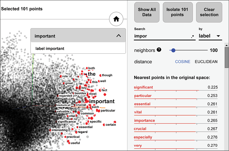
Figure 4.1: Visualization of nearest neighbors of the word “important” in a word embedding dataset, from the TensorFlow Embedding Guide (https://www.tensorflow.org/guide/embedding)

In the next section, we will look at various types of distributed representations (or word embeddings).

Static embeddings

Static embeddings are the oldest type of word embedding. The embeddings are generated against a large corpus but the number of words, though large, is finite. You can think of a static embedding as a dictionary, with words as the keys and their corresponding vector as the value. If you have a word whose embedding needs to be looked up that was not in the original corpus, then you are out of luck. In addition, a word has the same embedding regardless of how it is used, so static embeddings cannot address the problem of polysemy, that is, words with multiple meanings. We will explore this issue further when we cover non-static embeddings later in this chapter.

Word2Vec

The models known as Word2Vec were first created in 2013 by a team of researchers at Google led by Tomas Mikolov [1, 2, 3]. The models are self-supervised, that is, they are supervised models that depend on the structure of natural language to provide labeled training data.

The two architectures for Word2Vec are as follows:

• Continuous Bag of Words (CBOW)
• Skip-gram

Figure 4.2: Architecture of the CBOW and Skip-gram Word2Vec models

In the CBOW architecture, the model predicts the current word given a window of surrounding words. The order of context words does not influence the prediction (that is, the bag of words assumption, hence the name). In the skip-gram architecture, the model predicts the surrounding words given the context word. According to the Word2Vec website, CBOW is faster, but skip-gram does a better job at predicting infrequent words.

Figure 4.2 summarizes the CBOW and skip-gram architectures. To understand the inputs and outputs, consider the following example sentence:

The Earth travels around the Sun once per year.

Assuming a window size of 5, that is, two context words to the left and right of the content word, the resulting context windows are shown as follows. The word in bold is the word under consideration, and the other words are the context words within the window:

[_, _, The, Earth, travels]

[_, The, Earth, travels, around]

[The, Earth, travels, around, the]

[Earth, travels, around, the, Sun]

[travels, around, the, Sun, once]

[around, the, Sun, once, per]

[the, Sun, once, per, year]

[Sun, once, per, year, _]

[once, per, year, _, _]

For the CBOW model, the input and label tuples for the first three context windows are as follows. In the following first example, the CBOW model would learn to predict the word “The” given the set of words (“Earth,” “travels”), and so on. More correctly, the input of sparse vectors for the words “Earth” and “travels.” The model will learn to predict a dense vector whose highest value, or probability, corresponds to the word “The”:

([Earth, travels], The)

([The, travels, around], Earth)

([The, Earth, around, the], travels)

For the skip-gram model, the first three context windows correspond to the following input and label tuples. We can simplify the skip-gram model objective of predicting a context word given a target word to basically predicting if a pair of words are contextually related. Contextually related means that a pair of words within a context window are somehow related. That is, the input to the skip-gram model for the following first example would be the sparse vectors for the context words “The” and “Earth,” and the output would be the value 1:

([The, Earth], 1)

([The, travels], 1)

([Earth, The], 1)

([Earth, travels], 1)

([Earth, around], 1)

([travels, The], 1)

([travels, Earth], 1)

([travels, around], 1)

([travels, the], 1)

We also need negative samples to train a model properly, so we generate additional negative samples by pairing each input word with some random word in the vocabulary. This process is called negative sampling and might result in the following additional inputs:

([Earth, aardvark], 0)

([Earth, zebra], 0)

A model trained with all of these inputs is called a Skip-Gram with Negative Sampling (SGNS) model.

It is important to understand that we are not interested in the ability of these models to classify; rather, we are interested in the side effect of training – the learned weights. These learned weights are what we call the embedding.

While it may be instructive to implement the models on your own as an academic exercise, at this point Word2Vec is so commoditized, you are unlikely to ever need to do this. For the curious, you will find code to implement the CBOW and skip-gram models in the files tf2_cbow_model.py and tf2_cbow_skipgram.py in the source code accompanying this chapter.

The Word2Vec model was trained in a self-supervised manner by Google on roughly 100 billion words from the Google News dataset and contains a vocabulary of 3 million words. Google then released the pretrained model for anyone to download and use. The pretrained Word2Vec model is available here (https://drive.google.com/file/d/0B7XkCwpI5KDYNlNUTTlSS21pQmM/edit). The output vector dimensionality is 300. It is available as a BIN file and can be opened using Gensim by using gensim.models.Word2Vec.load_word2vec_format() or using the gensim() data downloader.

The other early implementation of word embedding is GloVe, which we will talk about next.

GloVe

The Global vectors for word representation (GloVe) embeddings were created by Jeffrey Pennington, Richard Socher, and Christopher Manning [4]. The authors describe GloVe as an unsupervised learning algorithm for obtaining vector representations for words. Training is performed on aggregated global word-word co-occurrence statistics from a corpus, and the resulting representations show similar clustering behavior between similar words as seen in Word2Vec.

GloVe differs from Word2Vec in that Word2Vec is a predictive model while GloVe is a count-based model. The first step is to construct a large matrix of (word, context) pairs that co-occur in the training corpus. Rows correspond to words and columns correspond to contexts, usually a sequence of one or more words. Each element of the matrix represents how often the word co-occurs in the context.

The GloVe process factorizes this co-occurrence matrix into a pair of (word, feature) and (feature, context) matrices. The process is known as matrix factorization and is done using Stochastic Gradient Descent (SGD), an iterative numerical method. For example, consider that we want to factorize a matrix R into its factors P and Q:

The SGD process will start with P and Q composed of random values and attempt to reconstruct the matrix R’ by multiplying them. The difference between the matrices R and R’ represents the loss and is usually computed as the mean-squared error between the two matrices. The loss dictates how much the values of P and Q need to change for R’ to move closer to R to minimize the reconstruction loss. This process is repeated multiple times until the loss is within some acceptable threshold. At that point, the (word, feature) matrix P is the GloVe embedding.

The GloVe process is much more resource-intensive than Word2Vec. This is because Word2Vec learns the embedding by training over batches of word vectors, while GloVe factorizes the entire co-occurrence matrix in one shot. In order to make the process scalable, SGD is often used in parallel mode, as outlined in the HOGWILD! paper [5].

Levy and Goldberg have also pointed out equivalences between the Word2Vec and GloVe approaches in their paper [6], showing that the Word2Vec SGNS model implicitly factorizes a word-context matrix.

As with Word2Vec, you are unlikely to ever need to generate your own GloVe embedding, and far more likely to use embeddings pre-generated against large corpora and made available for download. If you are curious, you will find code to implement matrix factorization in tf2_matrix_factorization.py in the source code download accompanying this chapter.

GloVe vectors trained on various large corpora (number of tokens ranging from 6 billion to 840 billion, vocabulary size from 400 thousand to 2.2 million) and of various dimensions (50, 100, 200, 300) are available from the GloVe project download page (https://nlp.stanford.edu/projects/glove/). It can be downloaded directly from the site or using Gensim or spaCy data downloaders.

Creating your own embeddings using Gensim

We will create an embedding using Gensim and a small text corpus, called text8.

Gensim is an open-source Python library designed to extract semantic meaning from text documents. One of its features is an excellent implementation of the Word2Vec algorithm, with an easy-to-use API that allows you to train and query your own Word2Vec model. To learn more about Gensim, see https://radimrehurek.com/gensim/index.html. To install Gensim, please follow the instructions at https://radimrehurek.com/gensim/install.html.

The text8 dataset is the first 10⁸ bytes of the Large Text Compression Benchmark, which consists of the first 10⁹ bytes of English Wikipedia [7]. The text8 dataset is accessible from within the Gensim API as an iterable of tokens, essentially a list of tokenized sentences. To download the text8 corpus, create a Word2Vec model from it, and save it for later use, run the following few lines of code (available in create_embedding_with_text8.py in the source code for this chapter):

import gensim.downloader as api
from gensim.models import Word2Vec
dataset = api.load("text8")
model = Word2Vec(dataset)
model.save("data/text8-word2vec.bin")

This will train a Word2Vec model on the text8 dataset and save it as a binary file. The Word2Vec model has many parameters, but we will just use the defaults. In this case, it trains a CBOW model (sg=0) with window size 5 (window=5) and will produce 100 dimensional embeddings (size=100). The full set of parameters is described on the Word2Vec documentation page [8]. To run this code, execute the following commands at the command line:

$ mkdir data
$ python create_embedding_with_text8.py

The code should run for 5-10 minutes, after which it will write out a trained model into the data folder. We will examine this trained model in the next section.

Exploring the embedding space with Gensim

Let us reload the Word2Vec model we just built and explore it using the Gensim API. The actual word vectors can be accessed as a custom Gensim class from the model’s wv attribute:

from gensim.models import KeyedVectors
model = KeyedVectors.load("data/text8-word2vec.bin")
word_vectors = model.wv

We can take a look at the first few words in the vocabulary and check to see if specific words are available:

words = word_vectors.vocab.keys()
print([x for i, x in enumerate(words) if i < 10])
assert("king" in words)

The preceding snippet of code produces the following output:

['anarchism', 'originated', 'as', 'a', 'term', 'of', 'abuse', 'first', 'used', 'against']

We can look for similar words to a given word (“king”), shown as follows:

def print_most_similar(word_conf_pairs, k):
   for i, (word, conf) in enumerate(word_conf_pairs):
       print("{:.3f} {:s}".format(conf, word))
       if i >= k-1:
           break
   if k < len(word_conf_pairs):
       print("...")
print_most_similar(word_vectors.most_similar("king"), 5)

The most_similar() method with a single parameter produces the following output. Here, the floating-point score is a measure of the similarity, higher values being better than lower values. As you can see, the similar words seem to be mostly accurate:

0.760 prince
0.701 queen
0.700 kings
0.698 emperor
0.688 throne
...

You can also do vector arithmetic similar to the country-capital example we described earlier. Our objective is to see if the relation Paris : France :: Berlin : Germany holds true. This is equivalent to saying that the distance in embedding space between Paris and France should be the same as that between Berlin and Germany. In other words, France - Paris + Berlin should give us Germany. In code, then, this would translate to:

print_most_similar(word_vectors.most_similar(
   positive=["france", "berlin"], negative=["paris"]), 1
)

This returns the following result, as expected:

0.803 germany

The preceding similarity value reported is cosine similarity, but a better measure of similarity was proposed by Levy and Goldberg [9], which is also implemented in the Gensim API. This measure essentially computes the distance on a log scale thereby amplifying the difference between shorter distances and reducing the difference between longer ones.

print_most_similar(word_vectors.most_similar_cosmul(
   positive=["france", "berlin"], negative=["paris"]), 1
)

And this also yields the expected result, but with higher similarity:

0.984 germany

Gensim also provides a doesnt_match() function, which can be used to detect the odd one out of a list of words:

print(word_vectors.doesnt_match(["hindus", "parsis", "singapore", "christians"]))

This gives us singapore as expected, since it is the only country among a set of words identifying religions.

We can also calculate the similarity between two words. Here we demonstrate that the distance between related words is less than that of unrelated words:

for word in ["woman", "dog", "whale", "tree"]:
   print("similarity({:s}, {:s}) = {:.3f}".format(
       "man", word,
       word_vectors.similarity("man", word)
   ))

This gives the following interesting result:

similarity(man, woman) = 0.759
similarity(man, dog) = 0.474
similarity(man, whale) = 0.290
similarity(man, tree) = 0.260

The similar_by_word() function is functionally equivalent to similar() except that the latter normalizes the vector before comparing by default. There is also a related similar_by_vector() function, which allows you to find similar words by specifying a vector as input. Here we try to find words that are similar to “singapore”:

print(print_most_similar(
   word_vectors.similar_by_word("singapore"), 5)
)

And we get the following output, which seems to be mostly correct, at least from a geographical point of view:

0.882 malaysia
0.837 indonesia
0.826 philippines
0.825 uganda
0.822 thailand
...

We can also compute the distance between two words in the embedding space using the distance() function. This is really just 1 - similarity():

print("distance(singapore, malaysia) = {:.3f}".format(
   word_vectors.distance("singapore", "malaysia")
))

We can also look up vectors for a vocabulary word either directly from the word_vectors object, or by using the word_vec() wrapper, shown as follows:

vec_song = word_vectors["song"]
vec_song_2 = word_vectors.word_vec("song", use_norm=True)

There are a few other functions that you may find useful depending on your use case. The documentation page for KeyedVectors contains a list of all the available functions [10].

The code shown here can be found in the explore_text8_embedding.py file in the code accompanying this book.

Using word embeddings for spam detection

Because of the widespread availability of various robust embeddings generated from large corpora, it has become quite common to use one of these embeddings to convert text input for use with machine learning models. Text is treated as a sequence of tokens. The embedding provides a dense fixed dimension vector for each token. Each token is replaced with its vector, and this converts the sequence of text into a matrix of examples, each of which has a fixed number of features corresponding to the dimensionality of the embedding.

This matrix of examples can be used directly as input to standard (non-neural network based) machine learning programs, but since this book is about deep learning and TensorFlow, we will demonstrate its use with a one-dimensional version of the Convolutional Neural Network (CNN) that you learned about in Chapter 3, Convolutional Neural Networks. Our example is a spam detector that will classify Short Message Service (SMS) or text messages as either “ham” or “spam.” The example is very similar to a sentiment analysis example we’ll cover in Chapter 20, Advanced Convolutional Neural Networks, that uses a one-dimensional CNN, but our focus here will be on the embedding layer.

Specifically, we will see how the program learns an embedding from scratch that is customized to the spam detection task. Next, we will see how to use an external third-party embedding like the ones we have learned about in this chapter, a process similar to transfer learning in computer vision. Finally, we will learn how to combine the two approaches, starting with a third-party embedding and letting the network use that as a starting point for its custom embedding, a process similar to fine-tuning in computer vision.

As usual, we will start with our imports:

import argparse
import gensim.downloader as api
import numpy as np
import os
import shutil
import tensorflow as tf
from sklearn.metrics import accuracy_score, confusion_matrix

Getting the data

The data for our model is available publicly and comes from the SMS spam collection dataset from the UCI Machine Learning Repository [11]. The following code will download the file and parse it to produce a list of SMS messages and their corresponding labels:

def download_and_read(url):
   local_file = url.split('/')[-1]
   p = tf.keras.utils.get_file(local_file, url,
       extract=True, cache_dir=".")
   labels, texts = [], []
   local_file = os.path.join("datasets", "SMSSpamCollection")
   with open(local_file, "r") as fin:
       for line in fin:
           label, text = line.strip().split('	')
           labels.append(1 if label == "spam" else 0)
           texts.append(text)
   return texts, labels
DATASET_URL = "https://archive.ics.uci.edu/ml/machine-learning-databases/00228/smsspamcollection.zip"
texts, labels = download_and_read(DATASET_URL)

The dataset contains 5,574 SMS records, 747 of which are marked as “spam” and the other 4,827 are marked as “ham” (not spam). The text of the SMS records is contained in the variable texts, and the corresponding numeric labels (0 = ham, 1 = spam) are contained in the variable labels.

Making the data ready for use

The next step is to process the data so it can be consumed by the network. The SMS text needs to be fed into the network as a sequence of integers, where each word is represented by its corresponding ID in the vocabulary. We will use the Keras tokenizer to convert each SMS text into a sequence of words, and then create the vocabulary using the fit_on_texts() method on the tokenizer.

We then convert the SMS messages to a sequence of integers using texts_to_sequences(). Finally, since the network can only work with fixed-length sequences of integers, we call the pad_sequences() function to pad the shorter SMS messages with zeros.

The longest SMS message in our dataset has 189 tokens (words). In many applications where there may be a few outlier sequences that are very long, we would restrict the length to a smaller number by setting the maxlen flag. In that case, sentences longer than maxlen tokens would be truncated, and sentences shorter than maxlen tokens would be padded:

# tokenize and pad text
tokenizer = tf.keras.preprocessing.text.Tokenizer()
tokenizer.fit_on_texts(texts)
text_sequences = tokenizer.texts_to_sequences(texts)
text_sequences = tf.keras.preprocessing.sequence.pad_sequences(
    text_sequences)
num_records = len(text_sequences)
max_seqlen = len(text_sequences[0])
print("{:d} sentences, max length: {:d}".format(
    num_records, max_seqlen))

We will also convert our labels to categorical or one-hot encoding format, because the loss function we would like to choose (categorical cross-entropy) expects to see the labels in that format:

# labels
NUM_CLASSES = 2
cat_labels = tf.keras.utils.to_categorical(
    labels, num_classes=NUM_CLASSES)

The tokenizer allows access to the vocabulary created through the word_index attribute, which is basically a dictionary of vocabulary words to their index positions in the vocabulary. We also build the reverse index that enables us to go from index position to the word itself. In addition, we create entries for the PAD character:

# vocabulary
word2idx = tokenizer.word_index
idx2word = {v:k for k, v in word2idx.items()}
word2idx["PAD"] = 0
idx2word[0] = "PAD"
vocab_size = len(word2idx)
print("vocab size: {:d}".format(vocab_size))

Finally, we create the dataset object that our network will work with. The dataset object allows us to set up some properties, such as the batch size, declaratively. Here, we build up a dataset from our padded sequence of integers and categorical labels, shuffle the data, and split it into training, validation, and test sets. Finally, we set the batch size for each of the three datasets:

# dataset
dataset = tf.data.Dataset.from_tensor_slices(
    (text_sequences, cat_labels))
dataset = dataset.shuffle(10000)
test_size = num_records // 4
val_size = (num_records - test_size) // 10
test_dataset = dataset.take(test_size)
val_dataset = dataset.skip(test_size).take(val_size)
train_dataset = dataset.skip(test_size + val_size)
BATCH_SIZE = 128
test_dataset = test_dataset.batch(BATCH_SIZE, drop_remainder=True)
val_dataset = val_dataset.batch(BATCH_SIZE, drop_remainder=True)
train_dataset = train_dataset.batch(BATCH_SIZE, drop_remainder=True)

Building the embedding matrix

The Gensim toolkit provides access to various trained embedding models, as you can see from running the following command at the Python prompt:

>>> import gensim.downloader as api
>>> api.info("models").keys()

This will return (at the time of writing this book) the following trained word embeddings:

• Word2Vec: Two flavors, one trained on Google news (3 million word vectors based on 3 billion tokens), and one trained on Russian corpora (word2vec-ruscorpora-300, word2vec-google-news-300).
• GloVe: Two flavors, one trained on the Gigawords corpus (400,000 word vectors based on 6 billion tokens), available as 50d, 100d, 200d, and 300d vectors, and one trained on Twitter (1.2 million word vectors based on 27 billion tokens), available as 25d, 50d, 100d, and 200d vectors (glove-wiki-gigaword-50, glove-wiki-gigaword-100, glove-wiki-gigaword-200, glove-wiki-gigaword-300, glove-twitter-25, glove-twitter-50, glove-twitter-100, glove-twitter-200). Smaller embedding sizes would result in greater compression of the input and consequently a greater degree of approximation.
• fastText: One million word vectors trained with subword information on Wikipedia 2017, the UMBC web corpus, and statmt.org news dataset (16B tokens) (fastText-wiki-news-subwords-300).
• ConceptNet Numberbatch: An ensemble embedding that uses the ConceptNet semantic network, the paraphrase database (PPDB), Word2Vec, and GloVe as input. Produces 600d vectors [12, 13].

For our example, we chose the 300d GloVe embeddings trained on the Gigaword corpus.

In order to keep our model size small, we want to only consider embeddings for words that exist in our vocabulary. This is done using the following code, which creates a smaller embedding matrix for each word in the vocabulary. Each row in the matrix corresponds to a word, and the row itself is the vector corresponding to the embedding for the word:

def build_embedding_matrix(sequences, word2idx, embedding_dim,
       embedding_file):
   if os.path.exists(embedding_file):
       E = np.load(embedding_file)
   else:
       vocab_size = len(word2idx)
       E = np.zeros((vocab_size, embedding_dim))
       word_vectors = api.load(EMBEDDING_MODEL)
       for word, idx in word2idx.items():
           try:
               E[idx] = word_vectors.word_vec(word)
           except KeyError:   # word not in embedding
               pass
       np.save(embedding_file, E)
   return E
EMBEDDING_DIM = 300
DATA_DIR = "data"
EMBEDDING_NUMPY_FILE = os.path.join(DATA_DIR, "E.npy")
EMBEDDING_MODEL = "glove-wiki-gigaword-300"
E = build_embedding_matrix(text_sequences, word2idx, 
   EMBEDDING_DIM,
   EMBEDDING_NUMPY_FILE)
print("Embedding matrix:", E.shape)

The output shape for the embedding matrix is (9010, 300), corresponding to the 9,010 tokens in the vocabulary, and 300 features in the third-party GloVe embeddings.

Defining the spam classifier

We are now ready to define our classifier. We will use a one-dimensional Convolutional Neural Network or ConvNet (1D CNN), similar to the network you have seen already in Chapter 3, Convolutional Neural Networks.

The input is a sequence of integers. The first layer is an embedding layer, which converts each input integer to a vector of size (embedding_dim). Depending on the run mode, that is, whether we will learn the embeddings from scratch, do transfer learning, or do fine-tuning, the embedding layer in the network would be slightly different. When the network starts with randomly initialized embedding weights (run_mode == "scratch") and learns the weights during the training, we set the trainable parameter to True. In the transfer learning case (run_mode == "vectorizer"), we set the weights from our embedding matrix E but set the trainable parameter to False, so it doesn’t train. In the fine-tuning case (run_mode == "finetuning"), we set the embedding weights from our external matrix E, as well as setting the layer to trainable.

The output of the embedding is fed into a convolutional layer. Here, fixed-size 3-token-wide 1D windows (kernel_size=3), also called time steps, are convolved against 256 random filters (num_filters=256) to produce vectors of size 256 for each time step. Thus, the output vector shape is (batch_size, time_steps, num_filters).

The output of the convolutional layer is sent to a 1D spatial dropout layer. Spatial dropout will randomly drop entire feature maps output from the convolutional layer. This is a regularization technique to prevent over-fitting. This is then sent through a global max pool layer, which takes the maximum value from each time step for each filter, resulting in a vector of shape (batch_size, num_filters).

The output of the dropout layer is fed into a pooling layer to flatten it, and then into a dense layer, which converts the vector of shape (batch_size, num_filters) to (batch_size, num_classes). A softmax activation will convert the scores for each of (spam, ham) into a probability distribution, indicating the probability of the input SMS being spam or ham respectively:

class SpamClassifierModel(tf.keras.Model):
   def __init__(self, vocab_sz, embed_sz, input_length,
           num_filters, kernel_sz, output_sz,
           run_mode, embedding_weights,
           **kwargs):
       super(SpamClassifierModel, self).__init__(**kwargs)
       if run_mode == "scratch":
           self.embedding = tf.keras.layers.Embedding(vocab_sz,
               embed_sz,
               input_length=input_length,
               trainable=True)
       elif run_mode == "vectorizer":
           self.embedding = tf.keras.layers.Embedding(vocab_sz,
               embed_sz,
               input_length=input_length,
               weights=[embedding_weights],
               trainable=False)
       else:
           self.embedding = tf.keras.layers.Embedding(vocab_sz,
               embed_sz,
               input_length=input_length,
               weights=[embedding_weights],
               trainable=True)
       self.conv = tf.keras.layers.Conv1D(filters=num_filters,
           kernel_size=kernel_sz,
           activation="relu")
       self.dropout = tf.keras.layers.SpatialDropout1D(0.2)
       self.pool = tf.keras.layers.GlobalMaxPooling1D()
       self.dense = tf.keras.layers.Dense(output_sz,
           activation="softmax")
   def call(self, x):
       x = self.embedding(x)
       x = self.conv(x)
       x = self.dropout(x)
       x = self.pool(x)
       x = self.dense(x)
       return x
# model definition
conv_num_filters = 256
conv_kernel_size = 3
model = SpamClassifierModel(
   vocab_size, EMBEDDING_DIM, max_seqlen,
   conv_num_filters, conv_kernel_size, NUM_CLASSES,
   run_mode, E)
model.build(input_shape=(None, max_seqlen))

Finally, we compile the model using the categorical cross entropy loss function and the Adam optimizer:

# compile
model.compile(optimizer="adam", loss="categorical_crossentropy", metrics=["accuracy"])

Training and evaluating the model

One thing to notice is that the dataset is somewhat imbalanced; there are only 747 instances of spam compared to 4,827 instances of ham. The network could achieve close to 87% accuracy simply by always predicting the majority class. To alleviate this problem, we set class weights to indicate that an error on a spam SMS is eight times as expensive as an error on a ham SMS. This is indicated by the CLASS_WEIGHTS variable, which is passed into the model.fit() call as an additional parameter.

After training for 3 epochs, we evaluate the model against the test set, and report the accuracy and confusion matrix of the model against the test set. However, for imbalance data, even with the use of class weights, the model may end up learning to always predict the majority class. Therefore, it is generally advisable to report accuracy on a per-class basis to make sure that the model learns to distinguish each class effectively. This can be done quite easily using the confusion matrix by dividing the diagonal element for each row by the sum of elements for that row, where each row corresponds to a labeled class:

NUM_EPOCHS = 3
# data distribution is 4827 ham and 747 spam (total 5574), which
# works out to approx 87% ham and 13% spam, so we take reciprocals
# and this works out to being each spam (1) item as being 
# approximately 8 times as important as each ham (0) message.
CLASS_WEIGHTS = { 0: 1, 1: 8 }
# train model
model.fit(train_dataset, epochs=NUM_EPOCHS,
   validation_data=val_dataset,
   class_weight=CLASS_WEIGHTS)
# evaluate against test set
labels, predictions = [], []
for Xtest, Ytest in test_dataset:
   Ytest_ = model.predict_on_batch(Xtest)
   ytest = np.argmax(Ytest, axis=1)
   ytest_ = np.argmax(Ytest_, axis=1)
   labels.extend(ytest.tolist())
   predictions.extend(ytest.tolist())
print("test accuracy: {:.3f}".format(accuracy_score(labels, predictions)))
print("confusion matrix")
print(confusion_matrix(labels, predictions))

Running the spam detector

The three scenarios we want to look at are:

• Letting the network learn the embedding for the task.
• Starting with a fixed external third-party embedding where the embedding matrix is treated like a vectorizer to transform the sequence of integers into a sequence of vectors.
• Starting with an external third-party embedding which is further fine-tuned to the task during the training.

Each scenario can be evaluated by setting the value of the mode argument as shown in the following command:

$ python spam_classifier --mode [scratch|vectorizer|finetune]

The dataset is small, and the model is fairly simple. We were able to achieve very good results (validation set accuracies in the high 90s, and perfect test set accuracy) with only minimal training (3 epochs). In all three cases, the network achieved a perfect score, accurately predicting the 1,111 ham messages, as well as the 169 spam cases.

The change in validation accuracies, shown in Figure 4.3, illustrates the differences between the three approaches:

Figure 4.3: Comparison of validation accuracy across training epochs for different embedding techniques

In the learning from scratch case, at the end of the first epoch, the validation accuracy is 0.93, but over the next two epochs, it rises to 0.98. In the vectorizer case, the network gets something of a head start from the third-party embeddings and ends up with a validation accuracy of almost 0.95 at the end of the first epoch. However, because the embedding weights are not allowed to change, it is not able to customize the embeddings to the spam detection task, and the validation accuracy at the end of the third epoch is the lowest among the three. The fine-tuning case, like the vectorizer, also gets a head start, but can customize the embedding to the task as well, and therefore is able to learn at the most rapid rate among the three cases. The fine-tuning case has the highest validation accuracy at the end of the first epoch and reaches the same validation accuracy at the end of the second epoch that the scratch case achieves at the end of the third.

In the next section, we will see that distributional similarity is not restricted to word embeddings; it applies to other scenarios as well.

Neural embeddings – not just for words

Word embedding technology has evolved in various ways since Word2Vec and GloVe. One such direction is the application of word embeddings to non-word settings, also known as neural embeddings. As you will recall, word embeddings leverage the distributional hypothesis that words occurring in similar contexts tend to have similar meanings, where context is usually a fixed-size (in number of words) window around the target word.

The idea of neural embeddings is very similar; that is, entities that occur in similar contexts tend to be strongly related to each other. The way in which these contexts are constructed is usually situation-dependent. We will describe two techniques here that are foundational and general enough to be applied easily to a variety of use cases.

Item2Vec

The Item2Vec embedding model was originally proposed by Barkan and Koenigstein [14] for the collaborative filtering use case, that is, recommending items to users based on purchases by other users that have similar purchase histories to this user. It uses items in a web-store as the “words” and the itemset (the sequence of items purchased by a user over time) as the “sentence” from which the “word context” is derived.

For example, consider the problem of recommending items to shoppers in a supermarket. Assume that our supermarket sells 5,000 items, so each item can be represented as a sparse one-hot encoded vector of size 5,000. Each user is represented by their shopping cart, which is a sequence of such vectors. Applying a context window similar to the one we saw in the Word2Vec section, we can train a skip-gram model to predict likely item pairs. The learned embedding model maps the items to a dense low-dimensional space where similar items are close together, which can be used to make similar item recommendations.

node2vec

The node2vec embedding model was proposed by Grover and Leskovec [15], as a scalable way to learn features for nodes in a graph. It learns an embedding of the structure of the graph by executing a large number of fixed-length random walks on the graph. The nodes are the “words” and the random walks are the “sentences” from which the “word context” is derived in node2vec.

The Something2Vec page [40] provides a comprehensive list of ways in which researchers have tried to apply the distributional hypothesis to entities other than words. Hopefully, this list will spark ideas for your own “Something2Vec” representation.

To illustrate how easy it is to create your own neural embedding, we will generate a node2vec-like model or, more accurately, a predecessor graph-based embedding called DeepWalk, proposed by Perozzi, et al. [42] for papers presented at the NeurIPS conference from 1987-2015, by leveraging word co-occurrence relationships between them.

The dataset is a 11,463 × 5,812 matrix of word counts, where the rows represent words, and columns represent conference papers. We will use this to construct a graph of papers, where an edge between two papers represents a word that occurs in both of them. Both node2vec and DeepWalk assume that the graph is undirected and unweighted. Our graph is undirected, since a relationship between a pair of papers is bidirectional. However, our edges could have weights based on the number of word co-occurrences between the two documents. For our example, we will consider any number of co-occurrences above 0 to be a valid unweighted edge.

As usual, we will start by declaring our imports:

import gensim
import logging
import numpy as np
import os
import shutil
import tensorflow as tf
from scipy.sparse import csr_matrix
from sklearn.metrics.pairwise import cosine_similarity
logging.basicConfig(format='%(asctime)s : %(levelname)s : %(message)s', level=logging.INFO)

The next step is to download the data from the UCI repository and convert it to a sparse term-document matrix, TD, then construct a document-document matrix E by multiplying the transpose of the term-document matrix by itself. Our graph is represented as an adjacency or edge matrix by the document-document matrix. Since each element represents a similarity between two documents, we will binarize the matrix E by setting any non-zero elements to 1:

DATA_DIR = "./data"
UCI_DATA_URL = "https://archive.ics.uci.edu/ml/machine-learning-databases/00371/NIPS_1987-2015.csv"
def download_and_read(url):
   local_file = url.split('/')[-1]
   p = tf.keras.utils.get_file(local_file, url, cache_dir=".")
   row_ids, col_ids, data = [], [], []
   rid = 0
   f = open(p, "r")
   for line in f:
       line = line.strip()
       if line.startswith(""","):
           # header
           continue
       # compute non-zero elements for current row
       counts = np.array([int(x) for x in line.split(',')[1:]])
       nz_col_ids = np.nonzero(counts)[0]
       nz_data = counts[nz_col_ids]
       nz_row_ids = np.repeat(rid, len(nz_col_ids))
       rid += 1
       # add data to big lists
       row_ids.extend(nz_row_ids.tolist())
       col_ids.extend(nz_col_ids.tolist())
       data.extend(nz_data.tolist())
   f.close()
   TD = csr_matrix((
       np.array(data), (
           np.array(row_ids), np.array(col_ids)
           )
       ),
       shape=(rid, counts.shape[0]))
   return TD
# read data and convert to Term-Document matrix
TD = download_and_read(UCI_DATA_URL)
# compute undirected, unweighted edge matrix
E = TD.T * TD
# binarize
E[E > 0] = 1

Once we have our sparse binarized adjacency matrix, E, we can then generate random walks from each of the vertices. From each node, we construct 32 random walks of a maximum length of 40 nodes. The walks have a random restart probability of 0.15, which means that for any node, the particular random walk could end with a 15% probability. The following code will construct the random walks and write them out to a file given by RANDOM_WALKS_FILE. To give an idea of the input, we have provided a snapshot of the first 10 lines of this file, showing random walks starting from node 0:

0 1405 4845 754 4391 3524 4282 2357 3922 1667
0 1341 456 495 1647 4200 5379 473 2311
0 3422 3455 118 4527 2304 772 3659 2852 4515 5135 3439 1273
0 906 3498 2286 4755 2567 2632
0 5769 638 3574 79 2825 3532 2363 360 1443 4789 229 4515 3014 3683 2967 5206 2288 1615 1166
0 2469 1353 5596 2207 4065 3100
0 2236 1464 1596 2554 4021
0 4688 864 3684 4542 3647 2859
0 4884 4590 5386 621 4947 2784 1309 4958 3314
0 5546 200 3964 1817 845

Note that this is a very slow process. A copy of the output is provided along with the source code for this chapter in case you prefer to skip the random walk generation process:

NUM_WALKS_PER_VERTEX = 32
MAX_PATH_LENGTH = 40
RESTART_PROB = 0.15
RANDOM_WALKS_FILE = os.path.join(DATA_DIR, "random-walks.txt")
def construct_random_walks(E, n, alpha, l, ofile):
   if os.path.exists(ofile):
       print("random walks generated already, skipping")
       return
   f = open(ofile, "w")
   for i in range(E.shape[0]):  # for each vertex
       if i % 100 == 0:
           print("{:d} random walks generated from {:d} vertices"
               .format(n * i, i))
       for j in range(n):       # construct n random walks
           curr = i
           walk = [curr]
           target_nodes = np.nonzero(E[curr])[1]
           for k in range(l):   # each of max length l
               # should we restart?
               if np.random.random() < alpha and len(walk) > 5:
                   break
               # choose one outgoing edge and append to walk
               try:
                   curr = np.random.choice(target_nodes)
                   walk.append(curr)
                   target_nodes = np.nonzero(E[curr])[1]
               except ValueError:
                   continue
           f.write("{:s}
".format(" ".join([str(x) for x in walk])))
   print("{:d} random walks generated from {:d} vertices, COMPLETE"
       .format(n * i, i))
   f.close()
# construct random walks (caution: very long process!)
construct_random_walks(E, NUM_WALKS_PER_VERTEX, RESTART_PROB, MAX_PATH_LENGTH, RANDOM_WALKS_FILE)

A few lines from the RANDOM_WALKS_FILE are shown below. You could imagine that these look like sentences in a language where the vocabulary of words is all the node IDs in our graph. We have learned that word embeddings exploit the structure of language to generate a distributional representation for words. Graph embedding schemes such as DeepWalk and node2vec do the exact same thing with these “sentences” created out of random walks. Such embeddings can capture similarities between nodes in a graph that go beyond immediate neighbors, as we shall see:

0 1405 4845 754 4391 3524 4282 2357 3922 1667
0 1341 456 495 1647 4200 5379 473 2311
0 3422 3455 118 4527 2304 772 3659 2852 4515 5135 3439 1273
0 906 3498 2286 4755 2567 2632
0 5769 638 3574 79 2825 3532 2363 360 1443 4789 229 4515 3014 3683 2967 5206 2288 1615 1166
0 2469 1353 5596 2207 4065 3100
0 2236 1464 1596 2554 4021
0 4688 864 3684 4542 3647 2859
0 4884 4590 5386 621 4947 2784 1309 4958 3314
0 5546 200 3964 1817 845

We are now ready to create our word embedding model. The Gensim package offers a simple API that allows us to declaratively create and train a Word2Vec model, using the following code. The trained model will be serialized to the file given by W2V_MODEL_FILE. The Documents class allows us to stream large input files to train the Word2Vec model without running into memory issues. We will train the Word2Vec model in skip-gram mode with a window size of 10, which means we train it to predict up to five neighboring vertices given a central vertex. The resulting embedding for each vertex is a dense vector of size 128:

W2V_MODEL_FILE = os.path.join(DATA_DIR, "w2v-neurips-papers.model")
class Documents(object):
   def __init__(self, input_file):
       self.input_file = input_file
   def __iter__(self):
       with open(self.input_file, "r") as f:
           for i, line in enumerate(f):
               if i % 1000 == 0:
                   logging.info("{:d} random walks extracted".format(i))
               yield line.strip().split()
def train_word2vec_model(random_walks_file, model_file):
   if os.path.exists(model_file):
       print("Model file {:s} already present, skipping training"
           .format(model_file))
       return
   docs = Documents(random_walks_file)
   model = gensim.models.Word2Vec(
       docs,
       size=128,    # size of embedding vector
       window=10,   # window size
       sg=1,        # skip-gram model
       min_count=2,
       workers=4
   )
   model.train(
       docs,
       total_examples=model.corpus_count,
       epochs=50)
   model.save(model_file)
# train model
train_word2vec_model(RANDOM_WALKS_FILE, W2V_MODEL_FILE)

Our resulting DeepWalk model is just a Word2Vec model, so anything you can do with Word2Vec in the context of words, you can do with this model in the context of vertices. Let us use the model to discover similarities between documents:

def evaluate_model(td_matrix, model_file, source_id):
   model = gensim.models.Word2Vec.load(model_file).wv
   most_similar = model.most_similar(str(source_id))
   scores = [x[1] for x in most_similar]
   target_ids = [x[0] for x in most_similar]
   # compare top 10 scores with cosine similarity 
   # between source and each target
   X = np.repeat(td_matrix[source_id].todense(), 10, axis=0)
   Y = td_matrix[target_ids].todense()
   cosims = [cosine_similarity(X[i], Y[i])[0, 0] for i in range(10)]
   for i in range(10):
       print("{:d} {:s} {:.3f} {:.3f}".format(
           source_id, target_ids[i], cosims[i], scores[i]))
source_id = np.random.choice(E.shape[0])
evaluate_model(TD, W2V_MODEL_FILE, source_id)

The following output is shown. The first and second columns are the source and target vertex IDs. The third column is the cosine similarity between the term vectors corresponding to the source and target documents, and the fourth is the similarity score reported by the Word2Vec model. As you can see, cosine similarity reports a similarity only between 2 of the 10 document pairs, but the Word2Vec model is able to detect latent similarities in the embedding space. This is similar to the behavior we have noticed between one-hot encoding and dense embeddings:

src_id dst_id cosine_sim w2v_score
1971   5443        0.000     0.348
1971   1377        0.000     0.348
1971   3682        0.017     0.328
1971   51          0.022     0.322
1971   857         0.000     0.318
1971   1161        0.000     0.313
1971   4971        0.000     0.313
1971   5168        0.000     0.312
1971   3099        0.000     0.311
1971   462         0.000     0.310

The code for this embedding strategy is available in neurips_papers_node2vec.py in the source code folder accompanying this chapter. Next, we will move on to look at character and subword embeddings.

Character and subword embeddings

Another evolution of the basic word embedding strategy has been to look at character and subword embeddings instead of word embeddings. Character-level embeddings were first proposed by Xiang and LeCun [17] and have some key advantages over word embeddings.

First, a character vocabulary is finite and small – for example, a vocabulary for English would contain around 70 characters (26 characters, 10 numbers, and the rest special characters), leading to character models that are also small and compact. Second, unlike word embeddings, which provide vectors for a large but finite set of words, there is no concept of out-of-vocabulary for character embeddings, since any word can be represented by the vocabulary. Third, character embeddings tend to be better for rare and misspelled words because there is much less imbalance for character inputs than for word inputs.

Character embeddings tend to work better for applications that require the notion of syntactic rather than semantic similarity. However, unlike word embeddings, character embeddings tend to be task-specific and are usually generated inline within a network to support the task. For this reason, third-party character embeddings are generally not available.

Subword embeddings combine the idea of character and word embeddings by treating a word as a bag of character n-grams, that is, sequences of n consecutive words. They were first proposed by Bojanowski, et al. [18] based on research from Facebook AI Research (FAIR), which they later released as fastText embeddings. fastText embeddings are available for 157 languages, including English. The paper has reported state-of-the-art performance on a number of NLP tasks, especially word analogies and language tasks for languages with rich morphologies.

fastText computes embeddings for character n-grams where n is between 3 and 6 characters (default settings can be changed), as well as for the words themselves. For example, character n-grams for n=3 for the word “green” would be “<gr”, “gre”, “ree”, “een”, and “en>”. The beginning and end of words are marked with “<” and “>” characters respectively, to distinguish between short words and their n-grams such as “<cat>” and “cat”.

During lookup, you can look up a vector from the fastText embedding using the word as the key if the word exists in the embedding. However, unlike traditional word embeddings, you can still construct a fastText vector for a word that does not exist in the embedding. This is done by decomposing the word into its constituent trigram subwords as shown in the preceding example, looking up the vectors for the subwords, and then taking the average of these subword vectors. The fastText Python API [19] will do this automatically, but you will need to do this manually if you use other APIs to access fastText word embeddings, such as Gensim or NumPy.

Next up, we will look at dynamic embeddings.

Dynamic embeddings

So far, all the embeddings we have considered have been static; that is, they are deployed as a dictionary of words (and subwords) mapped to fixed dimensional vectors. The vector corresponding to a word in these embeddings is going to be the same regardless of whether it is being used as a noun or verb in the sentence, for example, the word “ensure” (the name of a health supplement when used as a noun, and to make certain when used as a verb). It also provides the same vector for polysemous words or words with multiple meanings, such as “bank” (which can mean different things depending on whether it co-occurs with the word “money” or “river”). In both cases, the meaning of the word changes depending on clues available in its context, the sentence. Dynamic embeddings attempt to use these signals to provide different vectors for words based on their context.

Dynamic embeddings are deployed as trained networks that convert your input (typically a sequence of one-hot vectors) into a lower-dimensional dense fixed-size embedding by looking at the entire sequence, not just individual words. You can either preprocess your input to this dense embedding and then use this as input to your task-specific network, or wrap the network and treat it similar to the tf.keras.layers.Embedding layer for static embeddings. Using a dynamic embedding network in this way is usually much more expensive compared to generating it ahead of time (the first option) or using traditional embeddings.

The earliest dynamic embedding was proposed by McCann, et al. [20], and was called Contextualized Vectors (CoVe). This involved taking the output of the encoder from the encoder-decoder pair of a machine translation network and concatenating it with word vectors for the same word.

You will learn more about seq2seq networks in the next chapter. The researchers found that this strategy improved the performance of a wide variety of NLP tasks.

Another dynamic embedding proposed by Peters, et al. [21], was Embeddings from Language Models (ELMo). ELMo computes contextualized word representations using character-based word representation and bidirectional Long Short-Term Memory (LSTM). You will learn more about LSTMs in the next chapter. In the meantime, a trained ELMo network is available from TensorFlow’s model repository TensorFlow Hub. You can access it and use it for generating ELMo embeddings as follows.

The full set of models available on TensorFlow Hub that are TensorFlow 2.0 compatible can be found on the TensorFlow Hub site for TensorFlow 2.0 [16]. Here I have used an array of sentences, where the model will figure out tokens by using its default strategy of tokenizing on whitespace:

import tensorflow as tf
import tensorflow_hub as hub
 
elmo = hub.load("https://tfhub.dev/google/elmo/3")
embeddings = elmo.signatures["default"](
    tf.constant([
      "i like green eggs and ham",
      "would you eat them in a box"
    ]))["elmo"]
print(embeddings.shape)

The output is (2, 7, 1024). The first index tells us that our input contained 2 sentences. The second index refers to the maximum number of words across all sentences, in this case, 7. The model automatically pads the output to the longest sentence. The third index gives us the size of the contextual word embedding created by ELMo; each word is converted to a vector of size (1024).

You can also integrate the ELMo embedding layer into your TF2 model by wrapping it in a tf.keras.KerasLayer adapter. In this simple model, the model will return the embedding for the entire string:

embed = hub.KerasLayer("https://tfhub.dev/google/elmo/3",input_shape=[], dtype=tf.string)
model = tf.keras.Sequential([embed])
embeddings = model.predict([
    "i i like green eggs and ham",
    "would you eat them in a box"
])
print(embeddings.shape)

Dynamic embeddings such as ELMo are able to provide different embeddings for the same word when used in different contexts and represent an improvement over static embeddings such as Word2Vec or GloVe. A logical next step is embeddings that represent larger units of text, such as sentences and paragraphs. This is what we will look at in the next section.

Sentence and paragraph embeddings

A simple, yet surprisingly effective solution for generating useful sentence and paragraph embeddings is to average the word vectors of their constituent words. Even though we will describe some popular sentence and paragraph embeddings in this section, it is generally always advisable to try averaging the word vectors as a baseline.

Sentence (and paragraph) embeddings can also be created in a task-optimized way by treating them as a sequence of words and representing each word using some standard word vector. The sequence of word vectors is used as input to train a network for some specific task. Vectors extracted from one of the later layers of the network just before the classification layer generally tend to produce a very good vector representation for the sequence. However, they tend to be very task-specific, and are of limited use as a general vector representation.

An idea for generating general vector representations for sentences that could be used across tasks was proposed by Kiros, et al. [22]. They proposed using the continuity of text from books to construct an encoder-decoder model that is trained to predict surrounding sentences given a sentence. The vector representation of a sequence of words constructed by an encoder-decoder network is typically called a “thought vector.” In addition, the proposed model works on a very similar basis to skip-gram, where we try to predict the surrounding words given a word. For these reasons, these sentence vectors were called skip-thought vectors. The project released a Theano-based model that could be used to generate embeddings from sentences. Later, the model was re-implemented with TensorFlow by the Google Research team [23]. The Skip-Thoughts model emits vectors of size (2048) for each sentence. Using the model is not very straightforward, but the README.md file on the repository [23] provides instructions if you would like to use it.

A more convenient source of sentence embeddings is the Google Universal Sentence Encoder, available on TensorFlow Hub. There are two flavors of the encoder in terms of implementation. The first flavor is fast but not so accurate and is based on the Deep Averaging Network (DAN) proposed by Iyer, et al. [24], which combines embeddings for words and bigrams and sends it through a fully connected network. The second flavor is much more accurate but slower and is based on the encoder component of the transformer network proposed by Vaswani, et al. [25]. We will cover the transformer network in more detail in Chapter 6, Transformers.

As with ELMo, the Google Universal Sentence Encoder can also be loaded from TensorFlow Hub into your TF2 code. Here is some code that calls it with two of our example sentences:

embed = hub.load("https://tfhub.dev/google/universal-sentence-encoder-large/4")
embeddings = embed([
"i like green eggs and ham",
"would you eat them in a box"
])["outputs"]
print(embeddings.shape)

The output is (2, 512); that is, each sentence is represented by a vector of size (512). It is important to note that the Google Universal Sentence Encoder can handle any length of word sequence—so you could legitimately use it to get word embeddings on one end as well as paragraph embeddings on the other. However, as the sequence length gets longer, the quality of the embeddings tends to get “diluted.”

A much earlier related line of work in producing embeddings for long sequences such as paragraphs and documents was proposed by Le and Mikolov [26] soon after Word2Vec was proposed. It is now known interchangeably as Doc2Vec or Paragraph2Vec. The Doc2Vec algorithm is an extension of Word2Vec that uses surrounding words to predict a word. In the case of Doc2Vec, an additional parameter, the paragraph ID, is provided during training. At the end of the training, the Doc2Vec network learns an embedding for every word and an embedding for every paragraph. During inference, the network is given a paragraph with some missing words. The network uses the known part of the paragraph to produce a paragraph embedding, then uses this paragraph embedding and the word embeddings to infer the missing words in the paragraph. The Doc2Vec algorithm comes in two flavors—the Paragraph Vectors - Distributed Memory (PV-DM) and Paragraph Vectors - Distributed Bag of Words (PV-DBOW), roughly analogous to CBOW and skip-gram in Word2Vec. We will not look at Doc2Vec further in this book, except to note that the Gensim toolkit provides prebuilt implementations that you can train with your own corpus.

Having looked at the different forms of static and dynamic embeddings, we will now switch gears a bit and look at language model-based embeddings.

Language model-based embeddings

Language model-based embeddings represent the next step in the evolution of word embeddings. A language model is a probability distribution over sequences of words. Once we have a model, we can ask it to predict the most likely next word given a particular sequence of words. Similar to traditional word embeddings, both static and dynamic, they are trained to predict the next word (or previous word as well, if the language model is bidirectional) given a partial sentence from the corpus. Training does not involve active labeling, since it leverages the natural grammatical structure of large volumes of text, so in a sense, this is a self-supervised learning process.

The main difference between a language model as a word embedding and more traditional embeddings is that traditional embeddings are applied as a single initial transformation on the data and are then fine-tuned for specific tasks. In contrast, language models are trained on large external corpora and represent a model of a particular language, say English. This step is called pretraining. The computing cost to pretrain these language models is usually fairly high; however, the people who pretrain these models generally make them available for use by others so we usually do not need to worry about this step. The next step is to fine-tune these general-purpose language models for your particular application domain. For example, if you are working in the travel or healthcare industry, you would fine-tune the language model with text from your own domain. Fine-tuning involves retraining the last few layers with your own text. Once fine-tuned, you can reuse this model for multiple tasks within your domain. The fine-tuning step is generally much less expensive compared to the pretraining step.

Once you have the fine-tuned language model, you remove the last layer of the language model and replace it with a one-to-two-layer fully connected network that converts the language model embedding for your input into the final categorical or regression output that your task needs. The idea is identical to transfer learning, which you learned about in Chapter 3, Convolutional Neural Networks, the only difference here is that you are doing transfer learning on text instead of images. As with transfer learning with images, these language model-based embeddings allow us to get surprisingly good results with very little labeled data. Not surprisingly, language model embeddings have been referred to as the “ImageNet moment” for natural language processing.

The language model-based embedding idea has its roots in the ELMo [21] network, which you have already seen in this chapter. ELMo learns about its language by being trained on a large text corpus to learn to predict the next and previous words given a sequence of words. ELMo is based on a bidirectional LSTM, which you will learn more about in Chapter 8, Autoencoders.

The first viable language model embedding was proposed by Howard and Ruder [27] via their Universal Language Model Fine-Tuning (ULMFiT) model, which was trained on the wikitext-103 dataset consisting of 28,595 Wikipedia articles and 103 million words. ULMFiT provides the same benefits that transfer learning provides for image tasks—better results from supervised learning tasks with comparatively less labeled data.

Meanwhile, the transformer architecture has become the preferred network for machine translation tasks, replacing the LSTM network because it allows for parallel operations and better handling of long-term dependencies. We will learn more about the transformer architecture in Chapter 6, Transformers. The OpenAI team of Radford, et al. [29] proposed using the decoder stack from the standard transformer network instead of the LSTM network used in ULMFiT. Using this, they built a language model embedding called Generative Pretraining (GPT) that achieved state of the art results for many language processing tasks. The paper proposes several configurations for supervised tasks involving single-and multi-sentence tasks such as classification, entailment, similarity, and multiple-choice question answering.

The OpenAI team later followed this up by building even larger language models called GPT-2 and GPT-3 respectively. GPT-2 was initially not released because of fears of misuse of the technology by malicious operators [30].

One problem with the OpenAI transformer architecture is that it is unidirectional whereas its predecessors ELMo and ULMFiT were bidirectional. Bidirectional Encoder Representations for Transformers (BERT), proposed by the Google AI team [28], uses the encoder stack of the Transformer architecture and achieves bidirectionality safely by masking up to 15% of its input, which it asks the model to predict.

As with the OpenAI paper, BERT proposes configurations for using it for several supervised learning tasks such as single- and multiple-sentence classification, question answering, and tagging.

The BERT model comes in two major flavors—BERT-base and BERT-large. BERT-base has 12 encoder layers, 768 hidden units, and 12 attention heads, with 110 million parameters in all. BERT-large has 24 encoder layers, 1,024 hidden units, and 16 attention heads, with 340 million parameters. More details can be found in the BERT GitHub repository [33].

BERT pretraining is an expensive process and can currently only be achieved using Tensor Processing Units (TPUs) or large distributed Graphics Processing Units (GPUs) clusters. TPUs are only available from Google via its Colab network [31] or Google Cloud Platform [32]. However, fine-tuning the BERT-base with custom datasets is usually achievable on GPU instances.

Once the BERT model is fine-tuned for your domain, the embeddings from the last four hidden layers usually produce good results for downstream tasks. Which embedding or combination of embeddings (via summing, averaging, max-pooling, or concatenating) to use is usually based on the type of task.

In the following section, we will look at how to extract embeddings from the BERT language model.

Using BERT as a feature extractor

The BERT project [33] provides a set of Python scripts that can be run from the command line to fine-tune BERT:

$ git clone https://github.com/google-research/bert.git
$ cd bert

We then download the appropriate BERT model we want to fine-tune. As mentioned earlier, BERT comes in two sizes—BERT-base and BERT-large. In addition, each model has a cased and uncased version. The cased version differentiates between upper and lowercase words, while the uncased version does not. For our example, we will use the BERT-base-uncased pretrained model. You can find the download URL for this and the other models further down the README.md page:

$ mkdir data
$ cd data
$ wget  
https://storage.googleapis.com/bert_models/2018_10_18/uncased_L-12_H-768_A-12.zip
$ unzip -a uncased_L-12_H-768_A-12.zip

This will create the following folder under the data directory of your local BERT project. The bert_config.json file is the configuration file used to create the original pretrained model, and the vocab.txt is the vocabulary used for the model, consisting of 30,522 words and word pieces:

uncased_L-12_H-768_A-12/
 ├── bert_config.json
 ├── bert_model.ckpt.data-00000-of-00001
 ├── bert_model.ckpt.index
 ├── bert_model.ckpt.meta
 └── vocab.txt

The pretrained language model can be directly used as a text feature extractor for simple machine learning pipelines. This can be useful for situations where you want to just vectorize your text input, leveraging the distributional property of embeddings to get a denser and richer representation than one-hot encoding.

The input in this case is just a file with one sentence per line. Let us call it sentences.txt and put it into our ${CLASSIFIER_DATA} folder. You can generate the embeddings from the last hidden layers by identifying them as -1 (last hidden layer), -2 (hidden layer before that), and so on. The command to extract BERT embeddings for your input sentences is as follows:

$ export BERT_BASE_DIR=./data/uncased_L-12_H-768_A-12
$ export CLASSIFIER_DATA=./data/my_data
$ export TRAINED_CLASSIFIER=./data/my_classifier
$ python extract_features.py 
    --input_file=${CLASSIFIER_DATA}/sentences.txt 
    --output_file=${CLASSIFIER_DATA}/embeddings.jsonl 
    --vocab_file=${BERT_BASE_DIR}/vocab.txt 
    --bert_config_file=${BERT_BASE_DIR}/bert_config.json 
    --init_checkpoint=${BERT_BASE_DIR}/bert_model.ckpt 
    --layers=-1,-2,-3,-4 
    --max_seq_length=128 
    --batch_size=8

The command will extract the BERT embeddings from the last four hidden layers of the model and write them out into a line-oriented JSON file called embeddings.jsonl in the same directory as the input file. These embeddings can then be used as input to downstream models that specialize in some specific task, such as sentiment analysis. Because BERT was pretrained on large quantities of English text, it learns a lot about the nuances of the language, which turn out to be useful for these downstream tasks. The downstream model does not have to be a neural network, it can be a non-neural model such as SVM or XGBoost as well.

There is much more you can do with BERT. The previous use case corresponds to transfer learning in computer vision. As in computer vision, it is also possible to fine-tune BERT (and other transformer models) for specific tasks, where the appropriate “head” network is attached to BERT, and the combined network is fine-tuned for a specific task. You will learn more about these techniques in Chapter 6, Transformers.

Summary

In this chapter, we have learned about the concepts behind distributional representations of words and their various implementations, starting from static word embeddings such as Word2Vec and GloVe.

We then looked at improvements to the basic idea, such as subword embeddings, sentence embeddings that capture the context of the word in the sentence, and the use of entire language models for generating embeddings. While language model-based embeddings are achieving state-of-the-art results nowadays, there are still plenty of applications where more traditional approaches yield very good results, so it is important to know them all and understand the tradeoffs.

We also looked briefly at other interesting uses of word embeddings outside the realm of natural language, where the distributional properties of other kinds of sequences are leveraged to make predictions in domains such as information retrieval and recommendation systems.

You are now ready to use embeddings, not only for your text-based neural networks, which we will look at in greater depth in the next chapter, but also in other areas of machine learning.

References

1. Mikolov, T., et al. (2013, Sep 7) Efficient Estimation of Word Representations in Vector Space. arXiv:1301.3781v3 [cs.CL].
2. Mikolov, T., et al. (2013, Sep 17). Exploiting Similarities among Languages for Machine Translation. arXiv:1309.4168v1 [cs.CL].
3. Mikolov, T., et al. (2013). Distributed Representations of Words and Phrases and their Compositionality. Advances in Neural Information Processing Systems 26 (NIPS 2013).
4. Pennington, J., Socher, R., Manning, C. (2014). GloVe: Global Vectors for Word Representation. D14-1162, Proceedings of the 2014 Conference on Empirical Methods in Natural Language Processing (EMNLP).
5. Niu, F., et al (2011, 11 Nov). HOGWILD! A Lock-Free Approach to Parallelizing Stochastic Gradient Descent. arXiv:1106.5730v2 [math.OC].
6. Levy, O., Goldberg, Y. (2014). Neural Word Embedding as Implicit Matrix Factorization. Advances in Neural Information Processing Systems 27 (NIPS 2014).
7. Mahoney, M. (2011, 1 Sep). text8 dataset: http://mattmahoney.net/dc/textdata.html
8. Rehurek, R. (2019, 10 Apr). gensim documentation for Word2Vec model: https://radimrehurek.com/gensim/models/word2vec.html
9. Levy, O., Goldberg, Y. (2014, 26-27 June). Linguistic Regularities in Sparse and Explicit Word Representations. Proceedings of the Eighteenth Conference on Computational Language Learning, pp 171-180 (ACL 2014).
10. Rehurek, R. (2019, 10 Apr). gensim documentation for KeyedVectors: https://radimrehurek.com/gensim/models/keyedvectors.html
11. Almeida, T. A., Gamez Hidalgo, J. M., and Yamakami, A. (2011). Contributions to the Study of SMS Spam Filtering: New Collection and Results. Proceedings of the 2011 ACM Symposium on Document Engineering (DOCENG): https://www.dt.fee.unicamp.br/~tiago/smsspamcollection/doceng11.pdf?ref=https://githubhelp.com
12. Speer, R., Chin, J. (2016, 6 Apr). An Ensemble Method to Produce High-Quality Word Embeddings. arXiv:1604.01692v1 [cs.CL].
13. Speer, R. (2016, 25 May). ConceptNet Numberbatch: a new name for the best Word Embeddings you can download: http://blog.conceptnet.io/posts/2016/conceptnet-numberbatch-a-new-name-for-the-best-word-embeddings-you-can-download/
14. Barkan, O., Koenigstein, N. (2016, 13-16 Sep). Item2Vec: Neural Item Embedding for Collaborative Filtering. IEEE 26th International Workshop on Machine Learning for Signal Processing (MLSP 2016).
15. Grover, A., Leskovec, J. (2016, 13-17 Aug). node2vec: Scalable Feature Learning for Networks. Proceedings of the 22nd ACM SIGKDD International Conference on Knowledge Discovery and Data Mining. (KDD 2016).
16. TensorFlow 2.0 Models on TensorFlow Hub: https://tfhub.dev/s?q=tf2-preview
17. Zhang, X., LeCun, Y. (2016, 4 Apr). Text Understanding from Scratch. arXiv 1502.01710v5 [cs.LG].
18. Bojanowski, P., et al. (2017, 19 Jun). Enriching Word Vectors with Subword Information. arXiv: 1607.04606v2 [cs.CL].
19. Facebook AI Research, fastText (2017). GitHub repository: https://github.com/facebookresearch/fastText
20. McCann, B., Bradbury, J., Xiong, C., Socher, R. (2017). Learned in Translation: Contextualized Word Vectors. Neural Information Processing Systems, 2017.
21. Peters, M., et al. (2018, 22 Mar). Deep contextualized word representations. arXiv: 1802.05365v2 [cs.CL].
22. Kiros, R., et al. (2015, 22 June). Skip-Thought Vectors. arXiv: 1506.06727v1 [cs.CL].
23. Kiros, R, et al (2017). GitHub repository: https://github.com/ryankiros/skip-thoughts
24. Iyer, M., Manjunatha, V., Boyd-Graber, J., Daume, H. (2015, July 26-31). Deep Unordered Composition Rivals Syntactic Methods for Text Classification. Proceedings of the 53rd Annual Meeting of the Association for Computational Linguistics and the 7th International Joint Conference on Natural Language Processing (ACL 2015).
25. Vaswani, A., et al. (2017, 6 Dec). Attention Is All You Need. arXiv: 1706.03762v5 [cs.CL].
26. Le, Q., Mikolov, T. (2014) Distributed Representation of Sentences and Documents. arXiv: 1405.4053v2 [cs.CL].
27. Howard, J., Ruder, S. (2018, 23 May). Universal Language Model Fine-Tuning for Text Classification. arXiv: 1801.06146v5 [cs.CL].
28. Devlin, J., Chang, M., Lee, K., Toutanova, K. (2018, 11 Oct). BERT: Pretraining of Deep Bidirectional Transformers for Language Understanding. arXiv: 1810.04805v1 [cs.CL]: https://arxiv.org/pdf/1810.04805.pdf
29. Radford, A., Narasimhan, K., Salimans, T., Sutskever, I. (2018). Improving Language Understanding with Unsupervised Learning: https://openai.com/blog/language-unsupervised/
30. Radford, A., et al. (2019). Language Models are unsupervised Multitask Learners. OpenAI Blog 2019: http://www.persagen.com/files/misc/radford2019language.pdf
31. Google Collaboratory: https://colab.research.google.com
32. Google Cloud Platform. https://cloud.google.com/
33. Google Research, BERT (2019). GitHub repository: https://github.com/google-research/bert
34. Nemeth (2019). Simple BERT using Tensorflow 2.0. Towards Data Science blog: https://towardsdatascience.com/simple-bert-using-tensorflow-2-0-132cb19e9b22
35. TF-IDF. Wikipedia. Retrieved May 2019: https://en.wikipedia.org/wiki/Tf%E2%80%93idf
36. Latent Semantic Analysis. Wikipedia. Retrieved May 2019: https://en.wikipedia.org/wiki/Latent_semantic_analysis
37. Topic Model. Wikipedia. Retrieved May 2019: https://en.wikipedia.org/wiki/Topic_model
38. Warstadt, A., Singh, A., and Bowman, S. (2018). Neural Network Acceptability Judgements. arXiv 1805:12471 [cs.CL]: https://nyu-mll.github.io/CoLA/
39. Microsoft Research Paraphrase Corpus. (2018): https://www.microsoft.com/en-us/download/details.aspx?id=52398
40. Nozawa, K. (2019). Something2Vec papers: https://gist.github.com/nzw0301/333afc00bd508501268fa7bf40cafe4e
41. Perrone, V., et al. (2016). Poisson Random Fields for Dynamic Feature Models: https://archive.ics.uci.edu/ml/datasets/NIPS+Conference+Papers+1987-2015
42. Perozzi, B., Al-Rfou, R., and Skiena, S. (2014). DeepWalk: Online Learning of Social Representations. arXiv 1403.6652v2 [cs.SI].

Join our book’s Discord space

Join our Discord community to meet like-minded people and learn alongside more than 2000 members at: https://packt.link/keras