3

Convolutional Neural Networks

In Chapter 1, Neural Network Foundations with TF, we discussed dense networks, in which each layer is fully connected to the adjacent layers. We looked at one application of those dense networks in classifying the MNIST handwritten characters dataset. In that context, each pixel in the input image has been assigned to a neuron for a total of 784 (28 x 28 pixels) input neurons. However, this strategy does not leverage the spatial structure and relationships between each image. In particular, this piece of code is a dense network that transforms the bitmap representing each written digit into a flat vector where the local spatial structure is removed. Removing the spatial structure is a problem because important information is lost:

#X_train is 60000 rows of 28x28 values --> reshaped in 60000 x 784
X_train = X_train.reshape(60000, 784)
X_test = X_test.reshape(10000, 784)

Convolutional neural networks leverage spatial information, and they are therefore very well-suited for classifying images. These nets use an ad hoc architecture inspired by biological data taken from physiological experiments performed on the visual cortex. Biological studies show that our vision is based on multiple cortex levels, each one recognizing more and more structured information. First, we see single pixels, then from that, we recognize simple geometric forms and then more and more sophisticated elements such as objects, faces, human bodies, animals, and so on.

Convolutional neural networks are a fascinating subject. Over a short period of time, they have shown themselves to be a disruptive technology, breaking performance records in multiple domains from text, to video, to speech, going well beyond the initial image processing domain where they were originally conceived. In this chapter, we will introduce the idea of convolutional neural networks (also known as CNNs, DCNNs, and ConvNets), a particular type of neural network that has large importance for deep learning.

This chapter covers the following topics:

• Deep convolutional neural networks
• An example of a deep convolutional neural network
• Recognizing CIFAR-10 images with deep learning
• Very deep convolutional networks for large-scale image recognition
• Deep Inception V3 networks for transfer learning
• Other CNN architectures
• Style transfer

Let’s begin with deep convolutional neural networks.

Deep convolutional neural networks

A Deep Convolutional Neural Network (DCNN) consists of many neural network layers. Two different types of layers, convolutional and pooling (i.e., subsampling), are typically alternated. The depth of each filter increases from left to right in the network. The last stage is typically made of one or more fully connected layers.

Figure 3.1: An example of a DCNN

There are three key underlying concepts for ConvNets: local receptive fields, shared weights, and pooling. Let’s review them together.

Local receptive fields

If we want to preserve the spatial information of an image or other form of data, then it is convenient to represent each image with a matrix of pixels. Given this, a simple way to encode the local structure is to connect a submatrix of adjacent input neurons into one single hidden neuron belonging to the next layer. That single hidden neuron represents one local receptive field. Note that this operation is named convolution, and this is where the name for this type of network is derived. You can think about convolution as the treatment of a matrix by another matrix, referred to as a kernel.

Of course, we can encode more information by having overlapping submatrices. For instance, let’s suppose that the size of every single submatrix is 5 x 5 and that those submatrices are used with MNIST images of 28 x 28 pixels. Then we will be able to generate 24 x 24 local receptive field neurons in the hidden layer. In fact, it is possible to slide the submatrices by only 23 positions before touching the borders of the images. In TensorFlow, the number of pixels along one edge of the kernel, or submatrix, is the kernel size, and the stride length is the number of pixels by which the kernel is moved at each step in the convolution.

Let’s define the feature map from one layer to another. Of course, we can have multiple feature maps that learn independently from each hidden layer. For example, we can start with 28 x 28 input neurons for processing MNIST images, and then define k feature maps of size 24 x 24 neurons each (again with shape of 5 x 5) in the next hidden layer.

Shared weights and bias

Let’s suppose that we want to move away from the pixel representation in a raw image, by gaining the ability to detect the same feature independently from the location where it is placed in the input image. A simple approach is to use the same set of weights and biases for all the neurons in the hidden layers. In this way, each layer will learn a set of position-independent latent features derived from the image, bearing in mind that a layer consists of a set of kernels in parallel, and each kernel only learns one feature.

A mathematical example

One simple way to understand convolution is to think about a sliding window function applied to a matrix. In the following example, given the input matrix I and the kernel K, we get the convolved output. The 3 x 3 kernel K (sometimes called the filter or feature detector) is multiplied elementwise with the input matrix to get one cell in the output matrix. All the other cells are obtained by sliding the window over I:

In this example, we decided to stop the sliding window as soon as we touch the borders of I (so the output is 3 x 3). Alternatively, we could have chosen to pad the input with zeros (so that the output would have been 5 x 5). This decision relates to the padding choice adopted. Note that kernel depth is equal to input depth (channel).

Another choice is about how far along we slide our sliding windows with each step. This is called the stride and it can be one or more. A larger stride generates fewer applications of the kernel and a smaller output size, while a smaller stride generates more output and retains more information.

The size of the filter, the stride, and the type of padding are hyperparameters that can be fine-tuned during the training of the network.

ConvNets in TensorFlow

In TensorFlow, if we want to add a convolutional layer with 32 parallel features and a filter size of 3x3, we write:

import tensorflow as tf
from tensorflow.keras import datasets, layers, models
model = models.Sequential()
model.add(layers.Conv2D(32, (3, 3), activation='relu', input_shape=(28, 28, 1)))

This means that we are applying a 3x3 convolution on 28x28 images with 1 input channel (or input filters) resulting in 32 output channels (or output filters).

An example of convolution is provided in Figure 3.2:

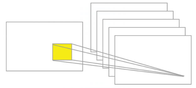
Figure.3.2: An example of convolution

Pooling layers

Let’s suppose that we want to summarize the output of a feature map. Again, we can use the spatial contiguity of the output produced from a single feature map and aggregate the values of a sub-matrix into one single output value synthetically describing the “meaning” associated with that physical region.

Max pooling

One easy and common choice is the so-called max pooling operator, which simply outputs the maximum activation as observed in the region. In Keras, if we want to define a max pooling layer of size 2 x 2, we write:

model.add(layers.MaxPooling2D((2, 2)))

An example of the max-pooling operation is given in Figure 3.3:

Figure 3.3: An example of max pooling

Average pooling

Another choice is average pooling, which simply aggregates a region into the average values of the activations observed in that region.

Note that Keras implements a large number of pooling layers, and a complete list is available online (see https://keras.io/layers/pooling/). In short, all the pooling operations are nothing more than a summary operation on a given region.

ConvNets summary

So far, we have described the basic concepts of ConvNets. CNNs apply convolution and pooling operations in one dimension for audio and text data along the time dimension, in two dimensions for images along the (height x width) dimensions, and in three dimensions for videos along the (height x width x time) dimensions. For images, sliding the filter over an input volume produces a map that provides the responses of the filter for each spatial position.

In other words, a ConvNet has multiple filters stacked together that learn to recognize specific visual features independently from the location in the image itself. Those visual features are simple in the initial layers of the network and become more and more sophisticated deeper in the network. Training of a CNN requires the identification of the right values for each filter so that an input, when passed through multiple layers, activates certain neurons of the last layer so that it will predict the correct values.

An example of DCNN: LeNet

Yann LeCun, who won the Turing Award, proposed [1] a family of ConvNets named LeNet, trained for recognizing MNIST handwritten characters with robustness to simple geometric transformations and distortion. The core idea of LeNet is to have lower layers alternating convolution operations with max-pooling operations. The convolution operations are based on carefully chosen local receptive fields with shared weights for multiple feature maps. Then, higher levels are fully connected based on a traditional MLP with hidden layers and softmax as the output layer.

LeNet code in TF

To define a LeNet in code, we use a convolutional 2D module (note that tf.keras.layers.Conv2D is an alias of tf.keras.layers.Convolution2D, so the two can be used in an interchangeable way – see https://www.tensorflow.org/api_docs/python/tf/keras/layers/Conv2D):

layers.Convolution2D(20, (5, 5), activation='relu', input_shape=input_shape)

where the first parameter is the number of output filters in the convolution and the next tuple is the extension of each filter. An interesting optional parameter is padding. There are two options: padding='valid' means that the convolution is only computed where the input and the filter fully overlap and therefore the output is smaller than the input, while padding='same' means that we have an output that is the same size as the input, for which the area around the input is padded with zeros.

In addition, we use a MaxPooling2D module:

layers.MaxPooling2D(pool_size=(2, 2), strides=(2, 2))

where pool_size=(2, 2) is a tuple of 2 integers representing the factors by which the image is vertically and horizontally downscaled. So (2, 2) will halve the image in each dimension, and strides=(2, 2) is the stride used for processing.

Now, let us review the code. First, we import a number of modules:

import tensorflow as tf
from tensorflow.keras import datasets, layers, models, optimizers
# network and training
EPOCHS = 5
BATCH_SIZE = 128
VERBOSE = 1
OPTIMIZER = tf.keras.optimizers.Adam()
VALIDATION_SPLIT=0.90
IMG_ROWS, IMG_COLS = 28, 28 # input image dimensions
INPUT_SHAPE = (IMG_ROWS, IMG_COLS, 1)
NB_CLASSES = 10  # number of outputs = number of digits

Then we define the LeNet network:

#define the convnet 
def build(input_shape, classes):
    model = models.Sequential()

We have a first convolutional stage with ReLU activations followed by max pooling. Our network will learn 20 convolutional filters, each one of which has a size of 5x5. The output dimension is the same as the input shape, so it will be 28 x 28. Note that since Convolutional2D is the first stage of our pipeline, we are also required to define its input_shape.

The max pooling operation implements a sliding window which slides over the layer and takes the maximum of each region with a step of two pixels both vertically and horizontally:

# CONV => RELU => POOL
model.add(layers.Convolution2D(20, (5, 5), activation='relu',
            input_shape=input_shape))
model.add(layers.MaxPooling2D(pool_size=(2, 2), strides=(2, 2)))

Then there is a second convolutional stage with ReLU activations, followed again by a max pooling layer. In this case, we increase the number of convolutional filters learned to 50 from the previous 20. Increasing the number of filters in deeper layers is a common technique in deep learning:

# CONV => RELU => POOL
model.add(layers.Convolution2D(50, (5, 5), activation='relu'))
model.add(layers.MaxPooling2D(pool_size=(2, 2), strides=(2, 2)))

Then we have a pretty standard flattening and a dense network of 500 neurons, followed by a softmax classifier with 10 classes:

# Flatten => RELU layers
model.add(layers.Flatten())
model.add(layers.Dense(500, activation='relu'))
# a softmax classifier
model.add(layers.Dense(classes, activation="softmax"))
return model

Congratulations, you have just defined your first deep convolutional learning network! Let’s see how it looks visually:

Figure 3.4: Visualization of LeNet

Now we need some additional code for training the network, but this is very similar to what we described in Chapter 1, Neural Network Foundations with TF. This time we also show the code for printing the loss:

# data: shuffled and split between train and test sets
(X_train, y_train), (X_test, y_test) = datasets.mnist.load_data()
# reshape
X_train = X_train.reshape((60000, 28, 28, 1))
X_test = X_test.reshape((10000, 28, 28, 1))
# normalize
X_train, X_test = X_train / 255.0, X_test / 255.0
# cast
X_train = X_train.astype('float32')
X_test = X_test.astype('float32')
# convert class vectors to binary class matrices
y_train = tf.keras.utils.to_categorical(y_train, NB_CLASSES)
y_test = tf.keras.utils.to_categorical(y_test, NB_CLASSES)
# initialize the optimizer and model
model = LeNet.build(input_shape=INPUT_SHAPE, classes=NB_CLASSES)
model.compile(loss="categorical_crossentropy", optimizer=OPTIMIZER,
    metrics=["accuracy"])
model.summary()
# use TensorBoard, princess Aurora!
callbacks = [
  # Write TensorBoard logs to './logs' directory
  tf.keras.callbacks.TensorBoard(log_dir='./logs')
]
# fit 
history = model.fit(X_train, y_train, 
        batch_size=BATCH_SIZE, epochs=EPOCHS, 
        verbose=VERBOSE, validation_split=VALIDATION_SPLIT,
        callbacks=callbacks)
score = model.evaluate(X_test, y_test, verbose=VERBOSE)
print("
Test score:", score[0])
print('Test accuracy:', score[1])

Now let’s run the code. As you can see in Figure 3.5, the time had a significant increase, and each iteration in our deep net now takes ~28 seconds against ~1-2 seconds for the network defined in Chapter 1, Neural Network Foundations with TF. However, the accuracy reached a new peak at 99.991% on training, 99.91% on validation, and 99.15% on test!

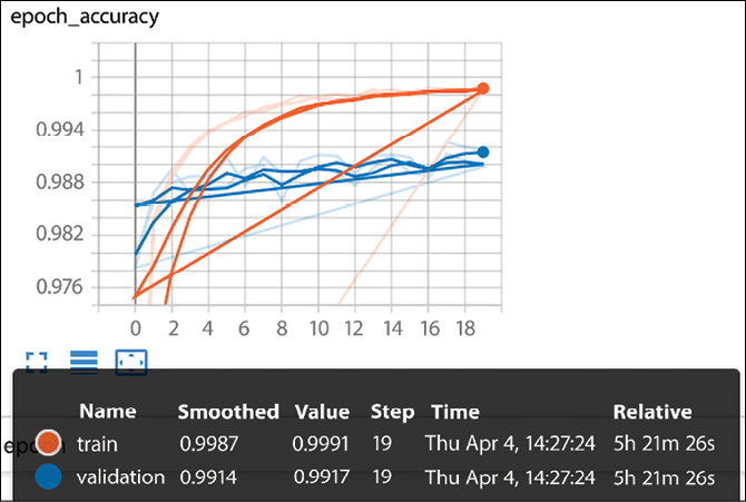
Figure 3.5: LeNet accuracy

Let’s see the execution of a full run for 20 epochs:

Model: "sequential_1"
_____________________________________________________________________
Layer (type)                    Output Shape              Param #    
=====================================================================
conv2d_2 (Conv2D)               (None, 24, 24, 20)        520        
                                                                     
max_pooling2d_2 (MaxPooling  2D) (None, 12, 12, 20)       0          
                                                                     
conv2d_3 (Conv2D)               (None, 8, 8, 50)          25050      
                                                                     
max_pooling2d_3 (MaxPooling  2D) (None, 4, 4, 50)         0          
                                                                     
flatten   (Flatten)             (None, 800)               0          
                                                                     
dense   (Dense)                 (None, 500)               400500     
                                                                     
dense_1 (Dense)                 (None, 10)                5010    
                                                                     
=====================================================================
Total params: 431,080
Trainable params: 431,080
Non-trainable params: 0
_________________________________________________________________
Train on 48000 samples, validate on 12000 samples
Epoch 1/20
[2019-04-04 14:18:28.546158: I tensorflow/core/profiler/lib/profiler_session.cc:164] Profile Session started.
48000/48000 [==============================] - 28s 594us/sample - loss: 0.2035 - accuracy: 0.9398 - val_loss: 0.0739 - val_accuracy: 0.9783
Epoch 2/20
48000/48000 [==============================] - 26s 534us/sample - loss: 0.0520 - accuracy: 0.9839 - val_loss: 0.0435 - val_accuracy: 0.9868
Epoch 3/20
48000/48000 [==============================] - 27s 564us/sample - loss: 0.0343 - accuracy: 0.9893 - val_loss: 0.0365 - val_accuracy: 0.9895
Epoch 4/20
48000/48000 [==============================] - 27s 562us/sample - loss: 0.0248 - accuracy: 0.9921 - val_loss: 0.0452 - val_accuracy: 0.9868
Epoch 5/20
48000/48000 [==============================] - 27s 562us/sample - loss: 0.0195 - accuracy: 0.9939 - val_loss: 0.0428 - val_accuracy: 0.9873
Epoch 6/20
48000/48000 [==============================] - 28s 548us/sample - loss: 0.0585 - accuracy: 0.9820 - val_loss: 0.1038 - val_accuracy: 0.9685
Epoch 7/20
48000/48000 [==============================] - 26s 537us/sample - loss: 0.0134 - accuracy: 0.9955 - val_loss: 0.0388 - val_accuracy: 0.9896
Epoch 8/20
48000/48000 [==============================] - 29s 589us/sample - loss: 0.0097 - accuracy: 0.9966 - val_loss: 0.0347 - val_accuracy: 0.9899
Epoch 9/20
48000/48000 [==============================] - 29s 607us/sample - loss: 0.0091 - accuracy: 0.9971 - val_loss: 0.0515 - val_accuracy: 0.9859
Epoch 10/20
48000/48000 [==============================] - 27s 565us/sample - loss: 0.0062 - accuracy: 0.9980 - val_loss: 0.0376 - val_accuracy: 0.9904
Epoch 11/20
48000/48000 [==============================] - 30s 627us/sample - loss: 0.0068 - accuracy: 0.9976 - val_loss: 0.0366 - val_accuracy: 0.9911
Epoch 12/20
48000/48000 [==============================] - 24s 505us/sample - loss: 0.0079 - accuracy: 0.9975 - val_loss: 0.0389 - val_accuracy: 0.9910
Epoch 13/20
48000/48000 [==============================] - 28s 584us/sample - loss: 0.0057 - accuracy: 0.9978 - val_loss: 0.0531 - val_accuracy: 0.9890
Epoch 14/20
48000/48000 [==============================] - 28s 580us/sample - loss: 0.0045 - accuracy: 0.9984 - val_loss: 0.0409 - val_accuracy: 0.9911
Epoch 15/20
48000/48000 [==============================] - 26s 537us/sample - loss: 0.0039 - accuracy: 0.9986 - val_loss: 0.0436 - val_accuracy: 0.9911
Epoch 16/20
48000/48000 [==============================] - 25s 513us/sample - loss: 0.0059 - accuracy: 0.9983 - val_loss: 0.0480 - val_accuracy: 0.9890
Epoch 17/20
48000/48000 [==============================] - 24s 499us/sample - loss: 0.0042 - accuracy: 0.9988 - val_loss: 0.0535 - val_accuracy: 0.9888
Epoch 18/20
48000/48000 [==============================] - 24s 505us/sample - loss: 0.0042 - accuracy: 0.9986 - val_loss: 0.0349 - val_accuracy: 0.9926
Epoch 19/20
48000/48000 [==============================] - 29s 599us/sample - loss: 0.0052 - accuracy: 0.9984 - val_loss: 0.0377 - val_accuracy: 0.9920
Epoch 20/20
48000/48000 [==============================] - 25s 524us/sample - loss: 0.0028 - accuracy: 0.9991 - val_loss: 0.0477 - val_accuracy: 0.9917
10000/10000 [==============================] - 2s 248us/sample - loss: 0.0383 - accuracy: 0.9915
Test score: 0.03832608199457617
Test accuracy: 0.9915

Let’s plot the model accuracy and the model loss, and we understand that we can train in only 10 iterations to achieve a similar accuracy of 99.1%:

Train on 48000 samples, validate on 12000 samples
Epoch 1/10
[2019-04-04 15:57:17.848186: I tensorflow/core/profiler/lib/profiler_session.cc:164] Profile Session started.
48000/48000 [==============================] - 26s 544us/sample - loss: 0.2134 - accuracy: 0.9361 - val_loss: 0.0688 - val_accuracy: 0.9783
Epoch 2/10
48000/48000 [==============================] - 30s 631us/sample - loss: 0.0550 - accuracy: 0.9831 - val_loss: 0.0533 - val_accuracy: 0.9843
Epoch 3/10
48000/48000 [==============================] - 30s 621us/sample - loss: 0.0353 - accuracy: 0.9884 - val_loss: 0.0410 - val_accuracy: 0.9874
Epoch 4/10
48000/48000 [==============================] - 37s 767us/sample - loss: 0.0276 - accuracy: 0.9910 - val_loss: 0.0381 - val_accuracy: 0.9887
Epoch 5/10
48000/48000 [==============================] - 24s 509us/sample - loss: 0.0200 - accuracy: 0.9932 - val_loss: 0.0406 - val_accuracy: 0.9881
Epoch 6/10
48000/48000 [==============================] - 31s 641us/sample - loss: 0.0161 - accuracy: 0.9950 - val_loss: 0.0423 - val_accuracy: 0.9881
Epoch 7/10
48000/48000 [==============================] - 29s 613us/sample - loss: 0.0129 - accuracy: 0.9955 - val_loss: 0.0396 - val_accuracy: 0.9894
Epoch 8/10
48000/48000 [==============================] - 27s 554us/sample - loss: 0.0107 - accuracy: 0.9965 - val_loss: 0.0454 - val_accuracy: 0.9871
Epoch 9/10
48000/48000 [==============================] - 24s 510us/sample - loss: 0.0082 - accuracy: 0.9973 - val_loss: 0.0388 - val_accuracy: 0.9902
Epoch 10/10
48000/48000 [==============================] - 26s 542us/sample - loss: 0.0083 - accuracy: 0.9970 - val_loss: 0.0440 - val_accuracy: 0.99892
10000/10000 [==============================] - 2s 196us/sample - loss: 0.0327 - accuracy: 0.9910
Test score: 0.03265062951518773
Test accuracy: 0.991

Let us see some of the MNIST images just to understand how good the number 99.1% is! For instance, there are many ways in which humans write a 9, one of them being in Figure 3.6. The same goes for 3, 7, 4, and 5, and number 1 in this figure is so difficult to recognize that even a human would likely have trouble:

Figure 3.6: An example of MNIST handwritten characters

We can summarize all the progress made so far with our different models in the following graph. Our simple net started with an accuracy of 90.71%, meaning that about 9 handwritten characters out of 100 are not correctly recognized. Then, we gained 8% with the deep learning architecture, reaching an accuracy of 99.2%, which means that less than one handwritten character out of one hundred is incorrectly recognized, as shown in Figure 3.7:

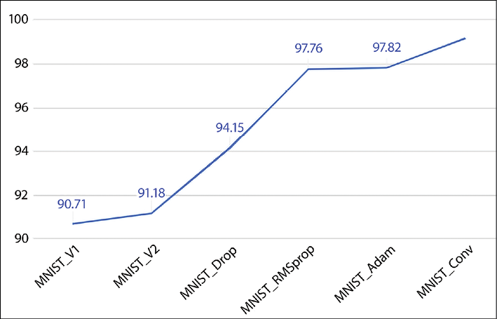
Figure 3.7: Accuracy for different models and optimizers

Understanding the power of deep learning

Another test we can run for a better understanding of the power of deep learning and ConvNets is to reduce the size of the training set and observe the resulting decay in performance. One way to do this is to split the training set of 50,000 examples into two different sets:

• The proper training set used for training our model will progressively reduce in size: 5,900, 3,000, 1,800, 600, and 300 examples.
• The validation set used to estimate how well our model has been trained will consist of the remaining examples. Our test set is always fixed, and it consists of 10,000 examples.

With this setup, we compare the previously defined deep learning ConvNet against the first example neural network defined in Chapter 1, Neural Network Foundations with TF. As we can see in the following graph, our deep network always outperforms the simple network when there is more data available. With 5,900 training examples, the deep learning net had an accuracy of 97.23% against an accuracy of 94% for the simple net.

In general, deep networks require more training data available to fully express their power, as shown in Figure 3.8:

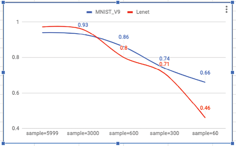
Figure 3.8: Accuracy for different amounts of data

A list of state-of-the-art results (for example, the highest performance available) for MNIST is available online (see http://rodrigob.github.io/are_we_there_yet/build/classification_datasets_results.html). As of March 2019, the best result has an error rate of 0.21% [2].

Recognizing CIFAR-10 images with deep learning

The CIFAR-10 dataset contains 60,000 color images of 32 x 32 pixels in three channels, divided into 10 classes. Each class contains 6,000 images. The training set contains 50,000 images, while the test set provides 10,000 images. This image taken from the CIFAR repository (see https://www.cs.toronto.edu/~kriz/cifar.html) shows a few random examples from the 10 classes:

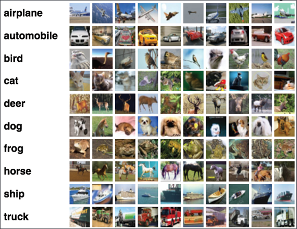
Figure 3.9: An example of CIFAR-10 images

The goal is to recognize previously unseen images and assign them to one of the ten classes. Let us define a suitable deep net.

First of all, we import a number of useful modules and define a few constants and load the dataset (the full code including the load operations is available online):

import tensorflow as tf
from tensorflow.keras import datasets, layers, models, optimizers
# CIFAR_10 is a set of 60K images 32x32 pixels on 3 channels
IMG_CHANNELS = 3
IMG_ROWS = 32
IMG_COLS = 32
#constant
BATCH_SIZE = 128
EPOCHS = 20
CLASSES = 10
VERBOSE = 1
VALIDATION_SPLIT = 0.2
OPTIM = tf.keras.optimizers.RMSprop()

Our net will learn 32 convolutional filters, each of which with a 3 x 3 size. The output dimension is the same as the input shape, so it will be 32 x 32 and the activation function used is a ReLU function, which is a simple way of introducing non-linearity. After that, we have a MaxPooling operation with a pool size of 2 x 2 and dropout at 25%:

#define the convnet 
def build(input_shape, classes):
    model = models.Sequential() 
    model.add(layers.Convolution2D(32, (3, 3), activation='relu',
                        input_shape=input_shape))
    model.add(layers.MaxPooling2D(pool_size=(2, 2)))
    model.add(layers.Dropout(0.25)) 

The next stage in the deep pipeline is a dense network with 512 units and ReLU activation followed by dropout at 50% and by a softmax layer with 10 classes as output, one for each category:

    model.add(layers.Flatten())
    model.add(layers.Dense(512, activation='relu'))
    model.add(layers.Dropout(0.5))
    model.add(layers.Dense(classes, activation='softmax'))
    return model

After defining the network, we can train the model. In this case, we split the data and compute a validation set in addition to the training and testing sets. The training is used to build our models, the validation is used to select the best-performing approach, while the test set is used to check the performance of our best models on fresh unseen data:

# use TensorBoard, princess Aurora!
callbacks = [
  # Write TensorBoard logs to './logs' directory
  tf.keras.callbacks.TensorBoard(log_dir='./logs')
]
# train
model.compile(loss='categorical_crossentropy', optimizer=OPTIM,
    metrics=['accuracy'])
 
model.fit(X_train, y_train, batch_size=BATCH_SIZE,
    epochs=EPOCHS, validation_split=VALIDATION_SPLIT, 
    verbose=VERBOSE, callbacks=callbacks) 
score = model.evaluate(X_test, y_test,
                     batch_size=BATCH_SIZE, verbose=VERBOSE)
print("
Test score:", score[0])
print('Test accuracy:', score[1])

Let’s run the code. Our network reaches a test accuracy of 66.8% with 20 iterations. We also print the accuracy and loss plot and dump the network with model.summary():

Epoch 17/20
40000/40000 [==============================] - 112s 3ms/sample - loss: 0.6282 - accuracy: 0.7841 - val_loss: 1.0296 - val_accuracy: 0.6734
Epoch 18/20
40000/40000 [==============================] - 76s 2ms/sample - loss: 0.6140 - accuracy: 0.7879 - val_loss: 1.0789 - val_accuracy: 0.6489
Epoch 19/20
40000/40000 [==============================] - 74s 2ms/sample - loss: 0.5931 - accuracy: 0.7958 - val_loss: 1.0461 - val_accuracy: 0.6811
Epoch 20/20
40000/40000 [==============================] - 71s 2ms/sample - loss: 0.5724 - accuracy: 0.8042 - val_loss: 0.1.0527 - val_accuracy: 0.6773
10000/10000 [==============================] - 5s 472us/sample - loss: 1.0423 - accuracy: 0.6686
Test score: 1.0423416819572449
Test accuracy: 0.6686

Figure 3.10 shows the accuracy and loss plot:

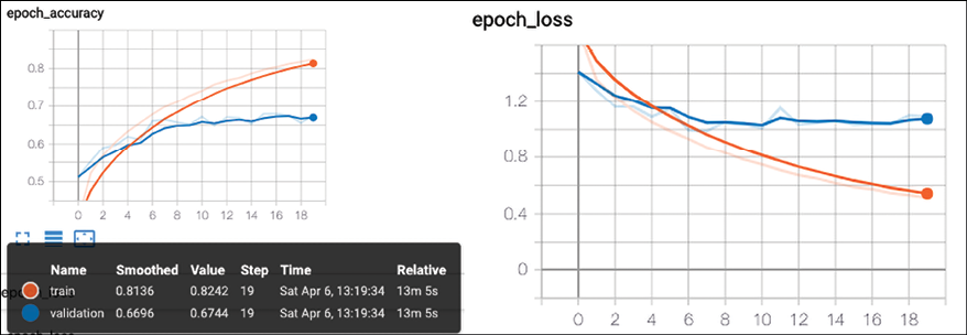
Figure 3.10: Accuracy and loss for the defined network

We have seen how to improve accuracy and how the loss changes for CIFAR-10 datasets. The next section is about improving the current results.

Improving the CIFAR-10 performance with a deeper network

One way to improve the performance is to define a deeper network with multiple convolutional operations. In the following example, we have a sequence of modules:

1st module: (CONV+CONV+MaxPool+DropOut)

2nd module: (CONV+CONV+MaxPool+DropOut)

3rd module: (CONV+CONV+MaxPool+DropOut)

These are followed by a standard dense output layer. All the activation functions used are ReLU functions. There is a new layer that we also discussed in Chapter 1, Neural Network Foundations with TF, BatchNormalization(), used to introduce a form of regularization between modules:

def build_model(): 
    model = models.Sequential()
    
    #1st block
    model.add(layers.Conv2D(32, (3,3), padding='same', 
        input_shape=x_train.shape[1:], activation='relu'))
    model.add(layers.BatchNormalization())
    model.add(layers.Conv2D(32, (3,3), padding='same', activation='relu'))
    model.add(layers.BatchNormalization())
    model.add(layers.MaxPooling2D(pool_size=(2,2)))
    model.add(layers.Dropout(0.2))
    #2nd block
    model.add(layers.Conv2D(64, (3,3), padding='same', activation='relu'))
    model.add(layers.BatchNormalization())
    model.add(layers.Conv2D(64, (3,3), padding='same', activation='relu'))
    model.add(layers.BatchNormalization())
    model.add(layers.MaxPooling2D(pool_size=(2,2)))
    model.add(layers.Dropout(0.3))
    #3d block 
    model.add(layers.Conv2D(128, (3,3), padding='same', activation='relu'))
    model.add(layers.BatchNormalization())
    model.add(layers.Conv2D(128, (3,3), padding='same', activation='relu'))
    model.add(layers.BatchNormalization())
    model.add(layers.MaxPooling2D(pool_size=(2,2)))
    model.add(layers.Dropout(0.4))
    #dense  
    model.add(layers.Flatten())
    model.add(layers.Dense(NUM_CLASSES, activation='softmax'))
    return model
    model.summary()

Congratulations! You have defined a deeper network. Let us run the code for 40 iterations reaching an accuracy of 82%! Let’s add the remaining part of the code for the sake of completeness. The first part is to load and normalize the data:

import tensorflow as tf
from tensorflow.keras import datasets, layers, models, regularizers, optimizers
from tensorflow.keras.preprocessing.image import ImageDataGenerator
import numpy as np
 
EPOCHS=50
NUM_CLASSES = 10
def load_data():
    (x_train, y_train), (x_test, y_test) = datasets.cifar10.load_data()
    x_train = x_train.astype('float32')
    x_test = x_test.astype('float32')
 
    #normalize 
    mean = np.mean(x_train,axis=(0,1,2,3))
    std = np.std(x_train,axis=(0,1,2,3))
    x_train = (x_train-mean)/(std+1e-7)
    x_test = (x_test-mean)/(std+1e-7)
 
    y_train =  tf.keras.utils.to_categorical(y_train,NUM_CLASSES)
    y_test =  tf.keras.utils.to_categorical(y_test,NUM_CLASSES)
    return x_train, y_train, x_test, y_test

Then we need to have a part to train the network:

(x_train, y_train, x_test, y_test) = load_data()
model = build_model()
model.compile(loss='categorical_crossentropy', 
            optimizer='RMSprop', 
            metrics=['accuracy'])
#train
batch_size = 64
model.fit(x_train, y_train, batch_size=batch_size,
    epochs=EPOCHS, validation_data=(x_test,y_test)) 
score = model.evaluate(x_test, y_test,
                     batch_size=batch_size)
print("
Test score:", score[0])
print('Test accuracy:', score[1])

So, we have an improvement of 15.14% with respect to the previous simpler deeper network.

Improving the CIFAR-10 performance with data augmentation

Another way to improve the performance is to generate more images for our training. The idea here is that we can take the standard CIFAR training set and augment this set with multiple types of transformation, including rotation, rescaling, horizontal or vertical flip, zooming, channel shift, and many more. Let’s see the code applied on the same network defined in the previous section:

from tensorflow.keras.preprocessing.image import ImageDataGenerator
#image augmentation
datagen = ImageDataGenerator(
    rotation_range=30,
    width_shift_range=0.2,
    height_shift_range=0.2,
    horizontal_flip=True,
    )
datagen.fit(x_train)

rotation_range is a value in degrees (0-180) for randomly rotating pictures; width_shift and height_shift are ranges for randomly translating pictures vertically or horizontally; zoom_range is for randomly zooming pictures; horizontal_flip is for randomly flipping half of the images horizontally; fill_mode is the strategy used for filling in new pixels that can appear after a rotation or a shift.

After augmentation we have generated many more training images starting from the standard CIFAR-10 set, as shown in Figure 3.11:

Figure.3.11: An example of image augmentation

Now we can apply this intuition directly for training. Using the same ConvNet defined before, we simply generate more augmented images, and then we train. For efficiency, the generator runs in parallel to the model. This allows an image augmentation on a CPU while training in parallel on a GPU. Here is the code:

#train
batch_size = 64
model.fit_generator(datagen.flow(x_train, y_train, batch_size=batch_size),
                    epochs=EPOCHS,
                    verbose=1,validation_data=(x_test,y_test))
#save to disk
model_json = model.to_json()
with open('model.json', 'w') as json_file:
    json_file.write(model_json)
model.save_weights('model.h5') 
#test
scores = model.evaluate(x_test, y_test, batch_size=128, verbose=1)
print('
Test result: %.3f loss: %.3f' % (scores[1]*100,scores[0])) 

Each iteration is now more expensive because we have more training data. Therefore, let’s run for 50 iterations only. We see that by doing this we reach an accuracy of 85.91%:

Epoch 46/50
50000/50000 [==============================] - 36s 722us/sample - loss: 0.2440 - accuracy: 0.9183 - val_loss: 0.4918 - val_accuracy: 0.8546
Epoch 47/50
50000/50000 [==============================] - 34s 685us/sample - loss: 0.2338 - accuracy: 0.9208 - val_loss: 0.4884 - val_accuracy: 0.8574
Epoch 48/50
50000/50000 [==============================] - 32s 643us/sample - loss: 0.2383 - accuracy: 0.9189 - val_loss: 0.5106 - val_accuracy: 0.8556
Epoch 49/50
50000/50000 [==============================] - 37s 734us/sample - loss: 0.2285 - accuracy: 0.9212 - val_loss: 0.5017 - val_accuracy: 0.8581
Epoch 49/50
50000/50000 [==============================] - 36s 712us/sample - loss: 0.2263 - accuracy: 0.9228 - val_loss: 0.4911 - val_accuracy: 0.8591
10000/10000 [==============================] - 2s 160us/sample - loss: 0.4911 - accuracy: 0.8591
Test score: 0.4911323667049408
Test accuracy: 0.8591

The results obtained during our experiments are summarized in the following figure:

Figure 3.12: Accuracy on CIFAR-10 with different networks. On the x-axis, we have the increasing number of iterations

A list of state-of-the-art results for CIFAR-10 is available online (see http://rodrigob.github.io/are_we_there_yet/build/classification_datasets_results.html). As of April 2019, the best result has an accuracy of 96.53% [3].

Predicting with CIFAR-10

Let’s suppose that we want to use the deep learning model we just trained for CIFAR-10 for a bulk evaluation of images. Since we saved the model and the weights, we do not need to train each time:

import numpy as np
import scipy.misc
from tensorflow.keras.models import model_from_json
from tensorflow.keras.optimizers import SGD
#load model
model_architecture = 'cifar10_architecture.json'
model_weights = 'cifar10_weights.h5'
model = model_from_json(open(model_architecture).read())
model.load_weights(model_weights)
#load images
img_names = ['cat-standing.jpg', 'dog.jpg']
imgs = [np.transpose(scipy.misc.imresize(scipy.misc.imread(img_name), (32, 32)),
                     (2, 0, 1)).astype('float32')
           for img_name in img_names]
imgs = np.array(imgs) / 255
# train
optim = SGD()
model.compile(loss='categorical_crossentropy', optimizer=optim,
    metrics=['accuracy'])
# predict 
predictions = model.predict_classes(imgs)
print(predictions)

Note that we use SciPy’s imread to load the images and then resize them to 32 × 32 pixels. The resulting image tensor has dimensions of (32, 32, 3). However, we want the color dimension to be first instead of last, so we take the transpose. After that, the list of image tensors is combined into a single tensor and normalized to be between 0 and 1.0.

Now let us get the prediction for a and for a . We get categories 3 (cat) and 5 (dog) as output as expected. We successfully created a ConvNet to classify CIFAR-10 images. Next, we will look at VGG16: a breakthrough in deep learning.

Very deep convolutional networks for large-scale image recognition

In 2014, an interesting contribution to image recognition was presented in the paper Very Deep Convolutional Networks for Large-Scale Image Recognition, K. Simonyan and A. Zisserman [4]. The paper showed that a significant improvement on the prior-art configurations can be achieved by pushing the depth to 16-19 weight layers. One model in the paper denoted as D or VGG16 had 16 deep layers. An implementation in Java Caffe (see http://caffe.berkeleyvision.org/) was used for training the model on the ImageNet ILSVRC-2012 (see http://image-net.org/challenges/LSVRC/2012/) dataset, which includes images of 1,000 classes, and is split into three sets: training (1.3M images), validation (50K images), and testing (100K images). Each image is (224 x 224) on 3 channels. The model achieves 7.5% top-5 error (the error of the top 5 results) on ILSVRC-2012-val and 7.4% top-5 error on ILSVRC-2012-test.

According to the ImageNet site:

The goal of this competition is to estimate the content of photographs for the purpose of retrieval and automatic annotation using a subset of the large hand-labeled ImageNet dataset (10,000,000 labeled images depicting 10,000+ object categories) as training. Test images will be presented with no initial annotation -- no segmentation or labels -- and algorithms will have to produce labelings specifying what objects are present in the images.

The weights learned by the model implemented in Caffe have been directly converted (https://gist.github.com/baraldilorenzo/07d7802847aaad0a35d3) in tf.Keras and can be used by preloading them into the tf.Keras model, which is implemented below, as described in the paper:

import tensorflow as tf
from tensorflow.keras import layers, models
# define a VGG16 network
def VGG_16(weights_path=None):
    model = models.Sequential()
    model.add(layers.ZeroPadding2D((1,1),input_shape=(224,224, 3)))
    model.add(layers.Convolution2D(64, (3, 3), activation='relu'))
    model.add(layers.ZeroPadding2D((1,1)))
    model.add(layers.Convolution2D(64, (3, 3), activation='relu'))
    model.add(layers.MaxPooling2D((2,2), strides=(2,2)))
    model.add(layers.ZeroPadding2D((1,1)))
    model.add(layers.Convolution2D(128, (3, 3), activation='relu'))
    model.add(layers.ZeroPadding2D((1,1)))
    model.add(layers.Convolution2D(128, (3, 3), activation='relu'))
    model.add(layers.MaxPooling2D((2,2), strides=(2,2)))
    model.add(layers.ZeroPadding2D((1,1)))
    model.add(layers.Convolution2D(256, (3, 3), activation='relu'))
    model.add(layers.ZeroPadding2D((1,1)))
    model.add(layers.Convolution2D(256, (3, 3), activation='relu'))
    model.add(layers.ZeroPadding2D((1,1)))
    model.add(layers.Convolution2D(256, (3, 3), activation='relu'))
    model.add(layers.MaxPooling2D((2,2), strides=(2,2)))
    model.add(layers.ZeroPadding2D((1,1)))
    model.add(layers.Convolution2D(512, (3, 3), activation='relu'))
    model.add(layers.ZeroPadding2D((1,1)))
    model.add(layers.Convolution2D(512, (3, 3), activation='relu'))
    model.add(layers.ZeroPadding2D((1,1)))
    model.add(layers.Convolution2D(512, (3, 3), activation='relu'))
    model.add(layers.MaxPooling2D((2,2), strides=(2,2)))
    model.add(layers.ZeroPadding2D((1,1)))
    model.add(layers.Convolution2D(512, (3, 3), activation='relu'))
    model.add(layers.ZeroPadding2D((1,1)))
    model.add(layers.Convolution2D(512, (3, 3), activation='relu'))
    model.add(layers.ZeroPadding2D((1,1)))
    model.add(layers.Convolution2D(512, (3, 3), activation='relu'))
    model.add(layers.MaxPooling2D((2,2), strides=(2,2)))
    model.add(layers.Flatten())
    #top layer of the VGG net
    model.add(layers.Dense(4096, activation='relu'))
    model.add(layers.Dropout(0.5))
    model.add(layers.Dense(4096, activation='relu'))
    model.add(layers.Dropout(0.5))
    model.add(layers.Dense(1000, activation='softmax'))
    if weights_path:
        model.load_weights(weights_path)
    return model

We have implemented a VGG16 network. Note that we could also have used tf.keras.applications.vgg16. to get the model and its weights directly. Here, I wanted to show how VGG16 works internally. Next, we are going to utilize it.

Recognizing cats with a VGG16 network

Now let us test the image of a .

Note that we are going to use predefined weights:

import cv2
im = cv2.resize(cv2.imread('cat.jpg'), (224, 224)).astype(np.float32)
#im = im.transpose((2,0,1))
im = np.expand_dims(im, axis=0)
# Test pretrained model
model = VGG_16('/Users/antonio/.keras/models/vgg16_weights_tf_dim_ordering_tf_kernels.h5')
model.summary()
model.compile(optimizer='sgd', loss='categorical_crossentropy')
out = model.predict(im)
print(np.argmax(out))

When the code is executed, the class 285 is returned, which corresponds (see https://gist.github.com/yrevar/942d3a0ac09ec9e5eb3a) to “Egyptian cat”:

Total params: 138,357,544
Trainable params: 138,357,544
Non-trainable params: 0
---------------------------------------------------------------
285

Impressive, isn’t it? Our VGG16 network can successfully recognize images of cats! An important step for deep learning. It is only seven years since the paper in [4], but that was a game-changing moment.

Utilizing the tf.Keras built-in VGG16 net module

tf.Keras applications are pre-built and pretrained deep learning models. The weights are downloaded automatically when instantiating a model and stored at ~/.keras/models/. Using built-in code is very easy:

import tensorflow as tf
from tensorflow.keras.applications.vgg16 import VGG16
import matplotlib.pyplot as plt
import numpy as np
import cv2
# pre built model with pre-trained weights on imagenet
model = VGG16(weights='imagenet', include_top=True)
model.compile(optimizer='sgd', loss='categorical_crossentropy')
# resize into VGG16 trained images' format
im = cv2.resize(cv2.imread('steam-locomotive.jpg'), (224, 224))
im = np.expand_dims(im, axis=0)
# predict
out = model.predict(im)
index = np.argmax(out)
print(index)
plt.plot(out.ravel())
plt.show()
#this should print 820 for steaming train

Now, let us consider a train, . If we run the code, we get 820 as a result, which is the ImageNet code for “steam locomotive.” Equally important, all the other classes have very weak support, as shown in Figure 3.13:

Figure 3.13: A steam train is the most likely outcome

To conclude this section, note that VGG16 is only one of the modules that are pre-built in tf.Keras. A full list of pretrained models is available online (see https://www.tensorflow.org/api_docs/python/tf/keras/applications).

Recycling pre-built deep learning models for extracting features

One very simple idea is to use VGG16, and more generally DCNN, for feature extraction. This code implements the idea by extracting features from a specific layer.

Note that we need to switch to the functional API since the sequential model only accepts layers:

import tensorflow as tf
from tensorflow.keras.applications.vgg16 import VGG16 
from tensorflow.keras import models
from tensorflow.keras.preprocessing import image
from tensorflow.keras.applications.vgg16 import preprocess_input
import numpy as np
import cv2
# prebuild model with pre-trained weights on imagenet
base_model = VGG16(weights='imagenet', include_top=True)
print (base_model)
for i, layer in enumerate(base_model.layers):
    print (i, layer.name, layer.output_shape)
# extract features from block4_pool block
model = models.Model(inputs=base_model.input, 
    outputs=base_model.get_layer('block4_pool').output)
img_path = 'cat.jpg'
img = image.load_img(img_path, target_size=(224, 224))
x = image.img_to_array(img)
x = np.expand_dims(x, axis=0)
x = preprocess_input(x)
# get the features from this block
features = model.predict(x)
print(features)

You might wonder why we want to extract the features from an intermediate layer in a DCNN. The reasoning is that as the network learns to classify images into categories, each layer learns to identify the features that are necessary to perform the final classification. Lower layers identify lower-order features such as color and edges, and higher layers compose these lower-order features into higher-order features such as shapes or objects. Hence, the intermediate layer has the capability to extract important features from an image, and these features are more likely to help in different kinds of classification.

This has multiple advantages. First, we can rely on publicly available large-scale training and transfer this learning to novel domains. Second, we can save time on expensive training. Third, we can provide reasonable solutions even when we don’t have a large number of training examples for our domain. We also get a good starting network shape for the task at hand, instead of guessing it.

With this, we will conclude the overview of VGG16 CNNs, the last deep learning model defined in this chapter.

Deep Inception V3 for transfer learning

Transfer learning is a very powerful deep learning technique that has applications in a number of different domains. The idea behind transfer learning is very simple and can be explained with an analogy. Suppose you want to learn a new language, say Spanish. Then it could be useful to start from what you already know in a different language, say English.

Following this line of thinking, computer vision researchers now commonly use pretrained CNNs to generate representations for novel tasks [1], where the dataset may not be large enough to train an entire CNN from scratch. Another common tactic is to take the pretrained ImageNet network and then fine-tune the entire network to the novel task. For instance, we can take a network trained to recognize 10 categories of music and fine-tune it to recognize 20 categories of movies.

Inception V3 is a very deep ConvNet developed by Google [2]. tf.Keras implements the full network, as described in Figure 3.14, and it comes pretrained on ImageNet. The default input size for this model is 299x299 on three channels:

Figure 3.14: The Inception V3 deep learning model

This skeleton example is inspired by a scheme available online (see https://keras.io/applications/). Let’s suppose we have a training dataset D in a different domain from ImageNet. D has 1,024 features in input and 200 categories in output. Let’s look at a code fragment:

import tensorflow as tf
from tensorflow.keras.applications.inception_v3 import InceptionV3
from tensorflow.keras.preprocessing import image
from tensorflow.keras import layers, models
# create the base pre-trained model
base_model = InceptionV3(weights='imagenet', include_top=False)

We use a trained Inception V3 model: we do not include the fully connected layer – the dense layer with 1,024 inputs – because we want to fine-tune on D. The preceding code fragment will download the pretrained weights on our behalf:

Downloading data from https://github.com/fchollet/deep-learning-models/releases/download/v0.5/inception_v3_weights_tf_dim_ordering_tf_kernels_notop.h5
87916544/87910968 [===========================] – 26s 0us/step

So, if you look at the last four layers (where include_top=True), you see these shapes:

# layer.name, layer.input_shape, layer.output_shape
('mixed10', [(None, 8, 8, 320), (None, 8, 8, 768), (None, 8, 8, 768), (None, 8, 8, 192)], (None, 8, 8, 2048))
('avg_pool', (None, 8, 8, 2048), (None, 1, 1, 2048))
('flatten', (None, 1, 1, 2048), (None, 2048))
('predictions', (None, 2048), (None, 1000))

When include_top=False, you are removing the last three layers and exposing the mixed_10 layer. The GlobalAveragePooling2D layer converts (None, 8, 8, 2048) to (None, 2048), where each element in the (None, 2048) tensor is the average value for each corresponding (8,8) subtensor in the (None, 8, 8, 2048) tensor. None means an unspecified dimension, which is useful if you define a placeholder:

x = base_model.output
# let's add a fully-connected layer as first layer
x = layers.Dense(1024, activation='relu')(x)
# and a logistic layer with 200 classes as last layer
predictions = layers.Dense(200, activation='softmax')(x)
# model to train
model = models.Model(inputs=base_model.input, outputs=predictions)

All the convolutional levels are pretrained, so we freeze them during the training of the full model:

# i.e. freeze all convolutional InceptionV3 layers
for layer in base_model.layers:
    layer.trainable = False

The model is then compiled and trained for a few epochs so that the top layers are trained. For the sake of simplicity, here we are omitting the training code itself:

# compile the model (should be done *after* setting layers to non-trainable)
model.compile(optimizer='rmsprop', loss='categorical_crossentropy')
# train the model on the new data for a few epochs
model.fit_generator(...)

Then, we freeze the top inception layers and fine-tune the other inception layers. In this example, we decide to freeze the first 172 layers (this is a tunable hyperparameter):

# we chose to train the top 2 inception blocks, i.e. we will freeze
# the first 172 layers and unfreeze the rest:
for layer in model.layers[:172]:
   layer.trainable = False
for layer in model.layers[172:]:
   layer.trainable = True

The model is then recompiled for fine-tuning optimization:

# we need to recompile the model for these modifications to take effect
# we use SGD with a low learning rate
from tensorflow.keras.optimizers import SGD
model.compile(optimizer=SGD(lr=0.0001, momentum=0.9), loss='categorical_crossentropy')
# we train our model again (this time fine-tuning the top 2 inception blocks
# alongside the top Dense layers
model.fit_generator(...)

Now we have a new deep network that reuses a standard Inception V3 network, but it is trained on a new domain D via transfer learning. Of course, there are many fine-tuning parameters for achieving good accuracy. However, we are now re-using a very large pretrained network as a starting point via transfer learning. In doing so, we can save the need for training on our machines by reusing what is already available in tf.Keras.

Other CNN architectures

In this section, we will discuss many other different CNN architectures, including AlexNet, residual networks, highwayNets, DenseNets, and Xception.

AlexNet

One of the first convolutional networks was AlexNet [4], which consisted of only eight layers; the first five were convolutional ones with max-pooling layers, and the last three were fully connected. AlexNet [4] is an article cited more than 35,000 times, which started the deep learning revolution (for computer vision). Then, networks started to become deeper and deeper. Recently, a new idea has been proposed.

Residual networks

Residual networks are based on the interesting idea of allowing earlier layers to be fed directly into deeper layers. These are the so-called skip connections (or fast-forward connections). The key idea is to minimize the risk of vanishing or exploding gradients for deep networks (see Chapter 8, Autoencoders).

The building block of a ResNet is called a “residual block” or “identity block,” which includes both forward and fast-forward connections. In this example (Figure 3.15), the output of an earlier layer is added to the output of a later layer before being sent into a ReLU activation function:

Figure 3.15: An example of image segmentation

HighwayNets and DenseNets

An additional weight matrix may be used to learn the skip weights and these models are frequently denoted as HighwayNets. Instead, models with several parallel skips are known as DenseNets [5]. It has been noticed that the human brain might have similar patterns to residual networks since the cortical layer VI neurons get input from layer I, skipping intermediary layers. In addition, residual networks can be faster to train than traditional CNNs since there are fewer layers to propagate through during each iteration (deeper layers get input sooner due to the skip connection). Figure 3.16 shows an example of a DenseNet (based on http://arxiv.org/abs/1608.06993):

Figure 3.16: An example of a DenseNet

Xception

Xception networks use two basic blocks: a depthwise convolution and a pointwise convolution. A depthwise convolution is the channel-wise n x n spatial convolution. Suppose an image has three channels, then we have three convolutions of n x n. A pointwise convolution is a 1 x 1 convolution. In Xception, an “extreme” version of an Inception module, we first use a 1 x 1 convolution to map cross-channel correlations, and then separately map the spatial correlations of every output channel as shown in Figure 3.17 (from https://arxiv.org/pdf/1610.02357.pdf):

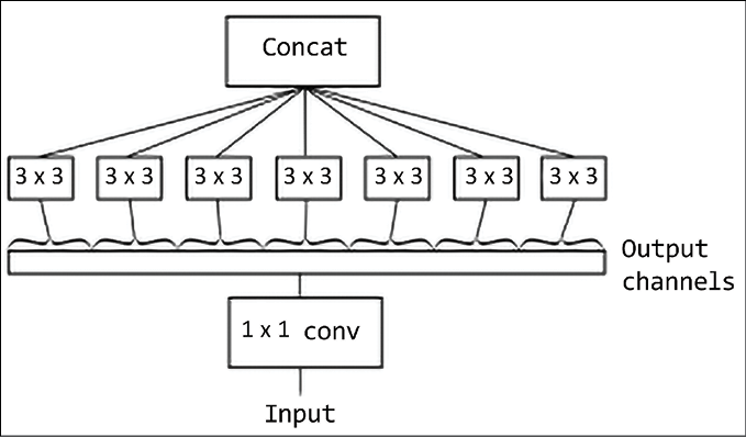
Figure 3.17: An example of an extreme form of an Inception module

Xception (eXtreme Inception) is a deep convolutional neural network architecture inspired by Inception, where Inception modules have been replaced with depthwise separable convolutions. Xception uses multiple skip-connections in a similar way to ResNet. The final architecture is rather complex as illustrated in Figure 3.18 (from https://arxiv.org/pdf/1610.02357.pdf). Data first goes through the entry flow, then through the middle flow, which is repeated eight times, and finally through the exit flow:

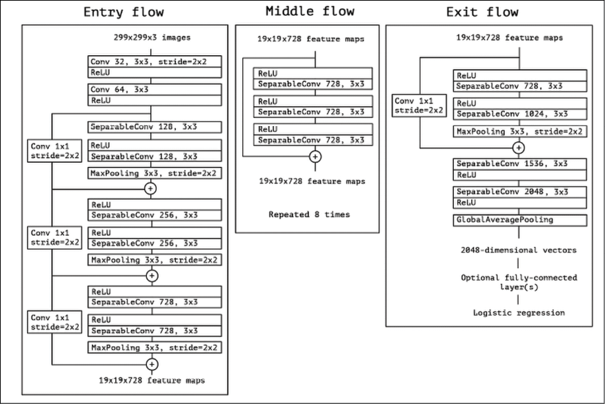
Figure 3.18: The full Xception architecture

Residual networks, HyperNets, DenseNets, Inception, and Xceptions are all available as pretrained nets in both tf.Keras.application and tf.Hub. The Keras website has a nice summary of the performance achieved on the ImageNet dataset and the depth of each network. The summary is available at https://keras.io/applications/:

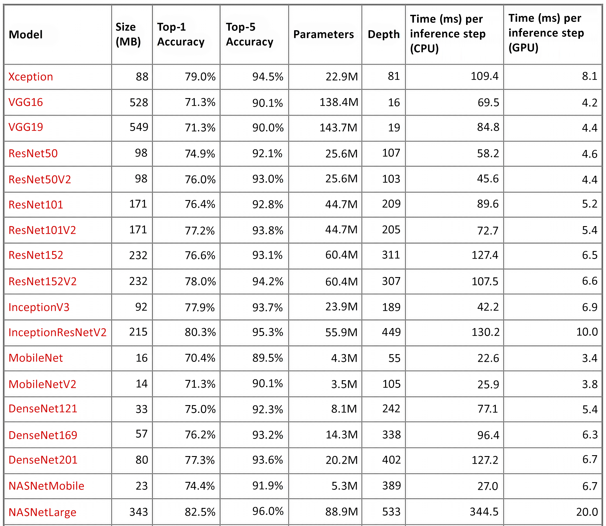
Figure 3.19: Different CNNs and accuracy on top-1 and top-5 results

The top-1 and top-5 accuracy refers to a model’s performance on the ImageNet validation dataset.

In this section, we have discussed many CNN architectures. The next section is about style transfer, a deep learning technique used for training neural networks to create art.

Style transfer

Style transfer is a funny neural network application that provides many insights into the power of neural networks. So what exactly is it? Imagine that you observe a painting done by a famous artist. In principle, you are observing two elements: the painting itself (say the face of a woman, or a landscape) and something more intrinsic, the “style” of the artist. What is the style? That is more difficult to define, but humans know that Picasso had his own style, Matisse had his own style, and each artist has his/her own style. Now, imagine taking a famous painting of Matisse, giving it to a neural network, and letting the neural network repaint it in Picasso’s style. Or, imagine taking your own photo, giving it to a neural network, and having your photo painted in Matisse’s or Picasso’s style, or in the style of any other artist that you like. That’s what style transfer does.

For instance, go to https://deepart.io/ and see a cool demo as shown in the image below, where deepart has been applied by taking the “Van Gogh” style as observed in the Sunflowers painting (this is a public domain image: “Sonnenblumen. Arles, 1888 Öl auf Leinwand, 92,5 x 73 cm Vincent van Gogh” https://commons.wikimedia.org/wiki/Vincent_van_Gogh#/media/File:Vincent_Van_Gogh_0010.jpg) and applying it to a picture of my daughter Aurora:

Figure 3.20: An example of deepart

Now, how can we define more formally the process of style transfer? Well, style transfer is the task of producing an artificial image x that shares the content of a source content image p and the style of a source style image a. So, intuitively we need two distance functions: one distance function measures how different the content of two images is, L_content, while the other distance function measures how different the style of two images is, L_style. Then, the transfer style can be seen as an optimization problem where we try to minimize these two metrics. As in A Neural Algorithm of Artistic Style by Leon A. Gatys, Alexander S. Ecker, and Matthias Bethge (https://arxiv.org/abs/1508.06576), we use a pretrained network to achieve style transfer. In particular, we can feed a VGG19 (or any suitable pretrained network) to extract features that represent images in an efficient way. Now we are going to define two functions used for training the network: the content distance and the style distance.

Content distance

Given two images, p content image and x input image, we define the content distance as the distance in the feature space defined by a layer l for a VGG19 network receiving the two images as an input. In other words, the two images are represented by the features extracted by a pretrained VGG19. These features project the images into a feature “content” space where the “content” distance can be conveniently computed as follows:

To generate nice images, we need to ensure that the content of the generated image is similar to (i.e. has a small distance from) that of the input image. The distance is therefore minimized with standard backpropagation. The code is simple:

#
#content distance
#
def get_content_loss(base_content, target):
  return tf.reduce_mean(tf.square(base_content - target))

Style distance

As discussed, the features in the higher layers of VGG19 are used as content representations. You can think about these features as filter responses. To represent the style we use in a gram matrix G (defined as the matrix v^Tv for a vector v), we consider as the inner matrix for map i and map j at layer l of the VGG19. It is possible to show that the Gram matrix represents the correlation matrix between different filter responses.

The contribution of each layer to the total style loss is defined as:

where is the Gram matrix for input image x and is the gram matrix for the style image a, and N_l is the number of feature maps, each of size . The Gram matrix can project the images into a space where the style is taken into account. In addition, the feature correlations from multiple VGG19 layers are used because we want to consider multi-scale information and a more robust style representation. The total style loss across levels is the weighted sum:

The key idea is therefore to perform gradient descent on the content image to make its style similar to the style image. The code is simple:

#style distance
#
def gram_matrix(input_tensor):
  # image channels first 
  channels = int(input_tensor.shape[-1])
  a = tf.reshape(input_tensor, [-1, channels])
  n = tf.shape(a)[0]
  gram = tf.matmul(a, a, transpose_a=True)
  return gram / tf.cast(n, tf.float32)
 
def get_style_loss(base_style, gram_target):
  # height, width, num filters of each layer
  height, width, channels = base_style.get_shape().as_list()
  gram_style = gram_matrix(base_style)
  
  return tf.reduce_mean(tf.square(gram_style - gram_target))

In short, the concepts behind style transfer are simple: first, we use VGG19 as a feature extractor and then we define two suitable function distances, one for style and the other one for contents, which are appropriately minimized. If you want to try this out for yourself, then TensorFlow tutorials are available online. A tutorial is available at https://colab.research.google.com/github/tensorflow/models/blob/master/research/nst_blogpost/4_Neural_Style_Transfer_with_Eager_Execution.ipynb. If you are interested in a demo of this technique, you can go to the deepart.io free site where they do style transfer.

Summary

In this chapter, we have learned how to use deep learning ConvNets to recognize MNIST handwritten characters with high accuracy. We used the CIFAR-10 dataset to build a deep learning classifier with 10 categories, and the ImageNet dataset to build an accurate classifier with 1,000 categories. In addition, we investigated how to use large deep learning networks such as VGG16 and very deep networks such as Inception V3. We concluded with a discussion on transfer learning.

In the next chapter, we’ll see how to work with word embeddings and why these techniques are important for deep learning.

References

1. LeCun, Y. and Bengio, Y. (1995). Convolutional networks for images, speech, and time series. The Handbook of Brain Theory Neural Networks, vol. 3361.
2. Wan. L, Zeiler M., Zhang S., Cun, Y. L., and Fergus R. (2014). Regularization of neural networks using dropconnect. Proc. 30th Int. Conf. Mach. Learn., pp. 1058–1066.
3. Graham B. (2014). Fractional Max-Pooling. arXiv Prepr. arXiv: 1412.6071.
4. Simonyan K. and Zisserman A. (Sep. 2014). Very Deep Convolutional Networks for Large-Scale Image Recognition. arXiv ePrints.

Join our book’s Discord space

Join our Discord community to meet like-minded people and learn alongside more than 2000 members at: https://packt.link/keras