20

Encapsulating DASP Technology

At present there are no external obstacles preventing beneficial exploitation of the digital alias-free signal processing technology on a relatively large scale. The existing microelectronic elements could be used for developing the hardware needed for that and there does not seems to be any problems with creating software. Actually this is not exactly correct. There are problems that complicate widespread application of the signal processing technology discussed in this book. Basically these are related to the fact that considerable expertise is required to be successful in this area and it is not very easy to acquire this. Substantial investments in terms of effort, time and money are needed to gain knowledge and experience sufficient to achieve really significant positive results. It is not realistic to expect that building such expertise can be done in many places quickly. A more rational and practical approach to widening the application field for this technology is based on the idea that the benefits in this area could be gained more easily by developing and exploiting application-specific subsystems for digital aliasfree signal processing. That clearly has to be done by embedding them in various larger IT systems operating as usual. This approach is discussed in this chapter. Among the gains immediately achievable in this way, widening of the digital domain in the direction of higher frequencies, simplification of data compression, complexity reduction of sensor arrays and achieving fault tolerance for signal processing could be mentioned. Issues essential for the development of the embedded systems capable of providing these benefits are discussed in this chapter in some detail.

20.1 Linking Digital Alias-free Signal Processing with Traditional Methods

To embed specific digital alias-free signal processing subsystems into larger conventional systems operating on the basis of equidistant data representation in the time domain, all specific features of the subsystems to be embedded should be encapsulated within them while their inputs and outputs are defined in a way fitting the standards of the respective embedding system. The advantage of this approach is obvious: there is no need to pay any attention to what happens inside the particular embedded system.

Various embedded DASP systems might be needed to cover a sufficiently wide application field. There could be universal and application-specific modifications. However, the variety of the embedded systems should be minimized while the application field covered by them is maximized. The complexity of the universal embedded systems capable of performing flexible signal processing in a wide application range could be much higher than the design complexity of the embedded systems applicable for fulfilling specific functions. These are much simpler by definition. Consequently, the expected operational speed of the specific embedded systems is typically much higher than the data processing rate achievable by the first class of systems. This fact increases the attractiveness of the specific embedded systems focused on fulfilling special functions. On the other hand, orientation towards specialized embedded systems leads to the necessity of having a longer list. To focus this discussion on the basic concepts of such embedded systems, the emphasis is put on a universal generic model.

20.1.1 Generic Model of the Embedded DASP Systems

Particular designs of the embedded DASP systems depend both on the microelectronic technology used for their implementation and on concepts underpinning them. Figure 20.1 illustrates a universal generic model of such an embedded system. It reflects the principles according to which this type of embedded system should be built in order to achieve their wide applicability for digital alias-free processing of various signals.

This version of the embedded DASP systems basically performs input signal encoding in an alias-free way and performs processing of the obtained digital signal in accordance with the algorithm used for programming the computer included in this scheme. The functional blocks inserted into the structure of this model are needed to fulfil a number of essential functions. One of the basic functions of the considered embedded DASP systems is to provide a dedicated service of converting input signals into their digital counterparts and representing them in a format meeting the requirements of the algorithms for their effective alias-free processing. Therefore they should have an analog input and a special pseudo-randomized ADC for performing nontraditional signal sampling and/or the quantizing procedure.

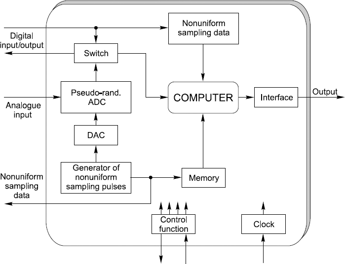
Figure 20.1 Structure of a generic embedded system for digital alias-free signal processing

The next block of particular significance is the computer. Capabilities of the embedded systems to a large extent depend on both the technical characteristics of the used computer and on the signal processing algorithms. It should also be realized that successful use of such embedded systems is possible only if signal processing is properly matched to the specifics of digitizing the signal. To ensure that, it is crucial to adapt processing of signals to the irregularities of sampling carried out at the stage of their digitizing. The information of the specific nonuniformities of the involved sampling process is kept in a memory and is used in the process of adapting signal processing operations to the signal sampling conditions.

While the embedded systems realized according to this generic model can be used for processing the input signals in many different ways, the following two operational modes can be described as the basic ones:

1. Signal analysis/synthesis. This operational mode is universal and very flexible. The essence of it is signal spectrum analysis with a following reconstruction of the input signal waveform and periodic resampling of it at a significantly increased frequency. This kind of signal processing requires relatively complicated iterative computations described in some detail in the following section. The problem is that the required calculations take a relatively long time and therefore it is not easy to achieve functioning of this system in real-time.
2. Signal vital parameter estimation. This second operational mode is also applicable in many cases. The point is that while waveforms of signals contain full information carried by them, only some parameters characterizing these waveforms often have to be estimated and used. Whenever this is the case, signal processing can be carried out in a way that is typically less complicated. This means that the programmable processors used for realizing this operational mode could provide the results substantially faster. In those cases, it is easier to achieve operation of this type of embedded system in real-time.

It may seem that these two operational modes differ substantially. In fact, this is often not true. Actually technical realization of the second operational mode might be simpler only in cases where some application-specific parameters characterizing some specific features of the signal are estimated. Whenever the parameters to be estimated are more universal, like the Fourier coefficients, amplitude and power, the complexity of both operational modes is approximately the same. This is so because it is crucial to adapt processing of nonuniformly sampled signals to the respective irregularities of the sampling process and the involved iterative procedure, basically determining the complexity of calculations, is based on direct and inverse Fourier transforms repeated several times in both cases.

In general, the role of the embedded systems for digital alias-free signal processing is to provide the dedicated service of digital processing of the input analog signal in a significantly widened frequency range, with representation of the output signal in a digital standard format that is normally and widely used to execute the standard instructions of traditional DSP algorithms. The DSP technology, well-developed over a long period of time, and the wealth of classic DSP algorithms, including algorithms for versatile digital filtering, could be fully used for further processing the signal digital waveforms and obtained signal parameter estimates whenever the described embedded systems could be and were used.

Incorporation of these universal embedded systems into traditional IT systems apparently leads to significant widening of the frequency range where signals could be processed fully digitally. However, other types of various significant benefits could be gained in this way as well.

20.1.2 Various DASP System Embedding Conditions

The conditions for matching inputs and outputs of the embedded DASP systems to the specifics of the traditional signal processing master systems obviously differ. Some of the variations most often met in conditions for application of the discussed embedded systems are considered.

Using Embedded Systems for Processing Pseudo-randomly Represented Signals of the Considered Type in Parallel

To connect specifically programmed embedded systems in parallel, a digital input/output is neeeded in addition to the analog input shown in Figure 20.1. According to this concept, the digital signal can be passed to the input of the processor either from the ADC output or from the digital input. In other applications, the digital signal formed by the ADC in an embedded system could be passed to other embedded systems used to fulfil additional signal processing tasks in parallel. A digital switch is included in the structures of these embedded systems in order to carry out these functions.

Encoding and Processing Several analog Signals in Parallel

So far encoding of only a single analog signal source has been considered. In many real-life situations there are a number of such sources. If the quantity of them is not too large, then the discussed universal embedded system is still applicable. The required number of these systems simply has to be used then or, in some other cases, the signal sources could be connected to a single embedded system of the considered type through a multiplexer.

Using Embedded Systems for Alias-Free Processing of a Large Quantity of analog Signals

Massive data acquisition and processing is not covered by the universal embedded system described above. A special approach to embedding systems performing the nonuniform procedures of signal encoding and preprocessing clearly has to be used in cases where data are acquired from a large number of signal sources. Although specific techniques have to be used in those cases, it still makes sense to use embedded systems as confined areas where the specifics of the digital alias-free signal processing are enclosed. The system illustrated by Figure 11.7 could be considered as an example of the embedded systems used to handle a large cluster of remotely sampled signals.

Achieving Complexity Reduction of Sensor Arrays

Using pseudo-randomized spatial and temporal signal encoding and processing is essential for achieving high performance at the array signal processing at a reduced quantity of sensors in the array. While it is of course essential to use embedded systems for encapsulation of specific nonuniform procedures for spatial and temporal spectrum analysis in this case, the fact has to be taken into account that a large amount of data is acquired from the sensors in the array and has to be processed as quickly as possible. Although, in principle, universal embedded systems built according to the above model could be used for pseudo-randomized spatial and temporal signal encoding and processing, better results could be expected if special types of embedded systems matched to the specifics of handling the array signals are developed and used.

Using Embedded Systems in Special Cases of Processing Distorted Periodic Sample Value Sequences

As shown in Sections 2.3 and 2.5, the algorithms and techniques developed specially for pseudo-randomized digitizing and processing of signals digitized in this special way could also be successfully used for reconstruction of impaired periodically sampled signals, achieving considerable fault tolerance, and for data compression executed in a simple manner. At first glance it seems that again specific embedded systems for digital alias-free signal processing need to be developed for applications in this area. However, more careful consideration of this matter has led to the conclusion that if only some minor changes are made in the structure of the universal embedded system then it could be used for these applications as well. Actually only a single functional block, specifically an analyser of sampling irregularities extracting the nonuniform sampling data, needs to be added to the structure shown in Figure 20.1. The task of this functional block is to analyse the digital input signals in these cases and to supply the processor with the information characterizing the specific sampling irregularities. This information can then be used to adapt signal processing to these specific sampling irregularities, as explained in the following sections. If this approach is used, no special embedded systems have to be developed and used for reconstruction of the compressed data and for reconstruction of data corrupted by interference or some other kind of functional fault.

20.2 Algorithm Options in the Development of Firmware

The essential functions of the considered embedded systems are signal alias-free digitizing, their representation in a digital format and waveform reconstruction. They are supported by hardware and firmware. Therefore the effectiveness of their application to a large extent depends on the methods and algorithms used as the basis for development of the embedded system firmware.

While there is little to be added to what has been said about signal pseudorandomized digitizing in previous chapters, less clear is the subject of quality achievable at signal representation in the frequency and time domains and at transforms of one particular type of signal representation into another one. The problem is that the classical approach to periodically sampled signal spectrum analysis and waveform reconstruction, based on direct and inverse Fourier transforms, is not fully applicable in the cases where the digital signals are given as sequences of sample values taken at pseudo-random time instants. The results of the DFT in those cases are distorted by errors due to sampling irregularities and therefore they do not represent the signal in the frequency domain sufficiently well. These errors have to be somehow filtered out, which is a difficult task. Discussions of the problems related to nonuniformly sampled signal representation in the frequency and time domains and a comparison of various approaches used to resolve them follow.

20.2.1 Sequential Exclusion of Signal Components

The basic problem with the spectrum analysis of nonuniformly sampled signals is the fact that errors in estimating parameters of a signal component in the frequency domain depend on the power of all other signal components. This dependence, of course, was noticed a long time ago but it took some time to develop a special algorithm for nonuniformly sampled signal processing that takes this fact into account. A successful approach to this problem was finally found. It is based on the use of the so-called sequential component extraction method, or SECOEX. Historically, development of the SECOEX method could be considered as a serious achievement marking progress gradually made in this area. The spectrum analysis of nonuniformly sampled signals performed on the basis of this algorithm demonstrated the fact that it is possible to improve significantly the results obtained at this stage of the DFT.

This method is based on estimating the most powerful of the signal components, taking it out of the original signal, then estimating the next most powerful component, subtracting it from the previously calculated difference and repeating these cyclic operations until the power of the reminder becomes smaller than a given threshold. More specifically, cyclic computations are carried out to optimize the following equation:

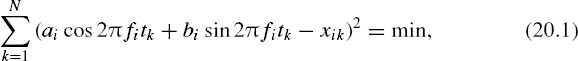
where the sample value set corresponding to the ith cycle is denoted by {x_ik}, i = 1, 2, 3,..., k = 1,..., N. To obtain {x_1k}, the most powerful signal component a₁ = A₁ sin ϕ₁; b₁ = A₁ cos ϕ₁ (A_i, ϕ_i and f_i are the amplitude, phase and frequency of the ith component respectively) has to be estimated and then subtracted from the digital input signal x(t_k) = x_k, k = 1,..., N. In general,

These operations are performed by estimating and varying all three parameters A_i, ϕ_i and f_i in accordance with Equation (20.1).

The algorithm developed on the basis of the SECOEX method suppresses relatively well the aliases present in the signal and the errors related to the crossinterference between the signal components. For example, the spectrogram shown in Figure 20.2(b) has been obtained using it. Compare this with the spectrogram displayed in Figure 20.2(a), which represents the results of the DFT performed for the same signal. It can be seen that application of SECOEX has improved the spectrogram significantly.

However, after a period of time it became clear that this method had some noticeable drawbacks and that it is possible to achieve more accurate results. Firstly, this method does not take into account the specific irregularities of the sampling instants at which the sample values of the respective signal are taken. Therefore it cannot be used as the basis for development of the processing procedures adaptable to the nonuniformities of the sampling process. Secondly, errors due to the cross-interference effect are not taken out completely. While taking out the larger components of the signal one by one effectively reduces the impact of the more powerful components on the estimation of the smaller components, the errors in the parameter estimation of the more powerful components are still enlarged as a result of the additive impact of the smaller components due to cross-interference. Thirdly, execution of the calculations arranged according to SECOEX is computationally burdensome. According to this approach, because the signal components are taken out sequentially, the Fourier coefficient estimates are calculated repeatedly in the whole frequency range of the respective signal for a number of times equal to the number of the most significant signal components.

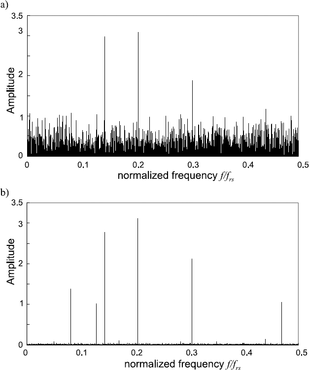
Figure 20.2 Spectrograms characterizing a nonuniformly sampled multitone signal obtained (a) as a result of the DFT and (b) by calculations made on the basis of the SECOEX method

20.2.2 Iterative Variable Threshold Calculations of DFT and IDFT

Another approach to improving the results of DFT could be used. Although it is also an iterative one, fewer iteration cycles are needed for realization of it. A group of signal components are estimated at each cycle rather than a single component, as in the case of SECOEX. Such an approach naturally leads to a reduction in the computational burden and to a saving of time.

A particular realization of this iterative method, based on using the FFT, could be used whenever the original is sampled pseudo-randomly with sampling instants located nonuniformly but on a well-defined time grid. Then the so-called zeropadding method could be used at the first cycle to transform the nonuniform sampling event stream into a periodic one, as briefly described in Section 15.3. Once that is done, the signal could be formally processed on the basis of the FFT.

The idea of using the FFT to obtain estimates of the Fourier coefficients is of course attractive as application of this fast algorithm drastically reduces the amount of calculations. However, using this approach evidently leads to large errors in estimating the Fourier coefficients. The achievable accuracy of these estimates is typically not acceptable. Therefore this procedure, if and when used, should be regarded as preliminary calculations providing only raw intermediate results. The degree of their usefulness depends on the used specific algorithm for signal analysis.

To suppress the errors due to sampling irregularities down to an acceptable level, a step-by-step approach should be used. The more powerful signal components are estimated at the first cycle. After that the second group of less powerful components are estimated and so on. Such an approach makes sense as the relative errors are smaller for the more powerful components. To realize it, a few threshold levels are introduced. The signal components above the upper threshold are estimated at the first cycle. Then the inverse DFT (IDFT) is carried out and the missing sample values are substituted by the corresponding instantaneous values of the roughly reconstructed waveform. After that the obtained signal sample value sequence is used for the repeated DFT. Significantly more accurate estimates of Fourier coefficients are obtained. At the next step, the threshold level is lowered and the components above it are estimated again. The process is continued in this way for a given number of cycles.

At first the DFT is performed for frequencies located on the frequency grid, with the interval between the frequencies determined by the signal observation time as usual. If all signal components are at frequencies located exactly on this grid, the DFT provides spectral estimates that are sufficiently accurate. However, the frequencies of real signal components are often shifted with regard to this grid. Then the positions of these components on the frequency axis have to be estimated more precisely. Otherwise the IDFT will result in unacceptable waveform reconstruction errors.

The IDFT is performed for all frequencies exceeding the mentioned thresholds. The waveform obtained as a result of the IDFT, performed for a number of the most powerful signal components, is given as

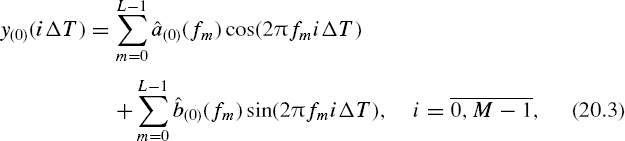
where L – 1 is the number of frequencies considered at the particular iteration cycle.

This waveform is periodically sampled with the sampling intervals equal to the step of the time grid. The initially used zeroes are then replaced by the taken sample values of this waveform. A periodic sequence of signal sample values is formed in this way. All actually taken signal sample values are in the right places and the roughly estimated sample values are inserted in the places initially occupied by zeroes. The precision of the signal digital representation can be significantly improved in this way. Therefore much more accurate estimates of the Fourier coefficients are obtained when the DFT is performed for this digital signal for the second time.

The following iteration cycles are repeated in an analogous way. Each time the threshold is put at a lower level and a group of previously not-estimated signal components, characterized by powers above this level, are estimated, this information is used for reducing the errors in signal sample value estimates at the time instants where the zeroes were placed at the beginning of the signal analysis process.

Relatively good results are obtained in this way. More will be said about this in Subsection 20.2.4. The main advantage of this iterative algorithm, in comparison with SECOEX, is the achieved possibility of using a significantly reduced number of iteration cycles. However, it is still not perfect. The basic drawback is related to the fact that the cross-interference strongly impacting the results of the DFT is not taken into account.

20.2.3 Algorithms Adapted to the Sampling Irregularities

There is no doubt that signal processing needs to be adapted to the nonuniformities of the involved sampling process whenever it is possible. As shown in Figure 20.1, such adapting is normally performed. The algorithms for this actually combine the adapting procedures with the iterative approach to cyclically repeated execution of the DFT and IDFT. In general, algorithms for signal processing adapted to the sampling irregularities are similar to the iterative algorithm discussed above. The basic difference is in the estimation of the Fourier coefficients for a group of signal components. While standard DFTs are used for this in the case of the described iterative algorithm, cross-interference coefficients are calculated and the effect of the cross-interference is taken into account in the case of the algorithm adapted to sampling irregularities. That changes the situation significantly. The precision of Fourier coefficient estimation is substantially increased at each iteration cycle, which leads to faster convergence to the final spectral estimates. Figure 20.3 illustrates this kind of adapted iterative signal processing.

It can be seen from Figure 20.3 that the estimation process develops quickly in this case. A more detailed comparison of this type of algorithm with both previously considered ones follows. Note that the illustrated spectrum analysis is actually only a part of the whole signal processing process. Each adaptation cycle contains calculations of direct and inverse DFTs. Therefore the signal waveform is also repeatedly estimated with growing precision.

For calculations carried out during the process of this adaptation, at each iteration cycle they typically cover a relatively small number of signal components at arbitrary frequencies. Under these conditions, the cross-interference coefficients, at separate adaptation cycles, are usually calculated for the particular group of peaks in the signal spectrum that is processed for this cycle. This means that it is then not necessary to calculate and use the matrix of the cross-interference coefficients characterizing the respective nonuniform sampling point process used to digitize the signal as described in Chapter 18. Direct on-line calculations of the cross-interference coefficients are then much more productive and the embedded systems shown in Figure 20.1 are based on this concept.

In cases where it is essential to achieve high operational speed, the discussed adaptation process could be realized in accordance with the scheme given in Figure 18.6. The used nonuniform sampling point process then has to be decomposed into a number of periodic processes with pseudo-randomly skipped sampling points. The signal sample values obtained at time instants defined by each particular sampling point substream can then be processed separately. In this way the sequential performance of a large number of required computational operations could be replaced by parallel calculations of reduced complexity carried out in parallel.

20.2.4 Comparison of Algorithm Performance

While all three types of the algorithms discussed above are applicable for adapting signal waveform reconstruction to the irregularities of the sampling process, their performance characteristics are different. To gain a first impression of their comparative qualities, a multitone test signal was digitized and its waveform was reconstructed in the presence of noise by applying all three algorithms. Diagrams of the SNR versus the iteration cycle numbers characterizing application of the three compared algorithms for signal waveform reconstruction are shown Figure 20.4. It can be seen from them that the waveform reconstruction errors, in the case where the reconstruction is performed on the basis of the SECOEX algorithm, decrease from one iterative cycle to the next relatively slowly and the iterative process is long. The second algorithm, the iterative algorithm, provides better results. However, the best results are obtained in the case of the third algorithm based on iteratively adapting the waveform reconstruction process to the sampling irregularities. When a signal waveform is reconstructed in accordance with this, suppression of the reconstruction error to their minimal value is achieved in a reduced number of iteration cycles.

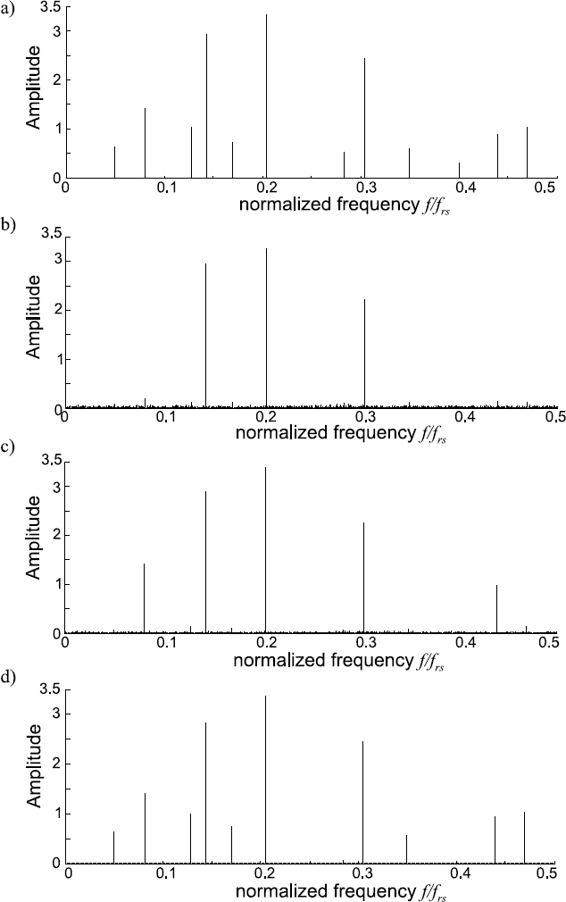
Figure 20.3 Results of spectrum analysis performed according to the iterative spectrum analysis adapted to the nonuniformities of the sampling process used when digitizing the signal: (a) true spectrogram; (b) spectrogram obtained at the end of the first cycle; (c) spectrogram after the second iteration; (d) spectrogram after the third iteration

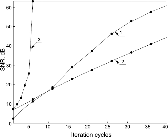
Figure 20.4 SNR versus the iteration cycle numbers characterizing application of the three compared algorithms for signal waveform reconstruction

20.3 Dedicated Services of the Embedded DASP Systems

According to the definition, embedded systems provide dedicated services to embedding systems. The services that should be offered by the embedded DASP systems are unusual, not paralleled by other types of embedded systems. Basically they need to widen significantly the frequency band within which the analog input signals can be fully processed digitally. More specifically, the dedicated services provided by them are based on the following functions:

• digitizing analog input signals in a way making it possible to avoid aliasinginduced errors at the following digital processing of these signals;
• performing signal digital preprocessing matched to the nonuniformities of the sampling process;
• presenting the results of digital preliminary processing of the signals into a form acceptable for the classic DSP hardware and software tools, which are used for further additional signal processing.

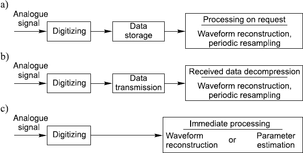
Figure 20.5 Typical dedicated services of the embedded DASP systems provided for digital processing of wideband analog signals

Some application hints are given in Figure 20.5 for the cases where the signals to be processed by the discussed embedded systems are analog. Firstly, these signals could be digitized, the digital versions of them stored in a memory and then processed when requested (Figure 20.5(a)). Note that the digital signal is typically encoded in a compressed form. Secondly, the digitized signals are transmitted over wire or wireless channels, received, demodulated and processed (Figure 20.5(b)). At least two embedded systems are obviously needed in that case. Thirdly, processing of the digitized signal is carried out without delay, preferably in the real-time processing mode, as illustrated by Figure 20.5(c).

Consider the suggested structure of this type of embedded system given in Figure 20.1. It is assumed that signal sample values are taken at time instants dictated by the generated pseudo-random sampling point process. This means that the signal sample value sequences processed by the computer are randomly decimated periodic sequences of numbers or, in other words, are periodic sequences of numbers with random skips. More often than not, the quantity of the missing numbers in these sequences is much larger than the quantity of the present numerical signal sample values.

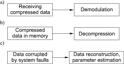
Figure 20.6 Typical dedicated services of the embedded DASP systems provided for processing of randomly decimated periodic digital signals

Now suppose that the computer processes the data given in the above form, reconstructs the signal waveform and presents it as a periodic sample value sequence with the period equal to the period characterizing the input data sequence. No signal sample values will then be missing. Compare the data flows at the computer input and output. Evidently the computer has decompressed the data given in a specifically compressed form. The performance of this function is representative of the kind of embedded system already discussed, so the role of the computer in the considered type of embedded system can often be defined in this way.

As the reconstruction of compressed data is a function of considerable practical value, it makes sense to use the embedded DASP systems, in addition to exploitation of them for dealing with analog signals, to process specifically presented digital signals. This is the reason why the digital inputs and some additional functional blocks are included in the structural scheme shown in Figure 20.1. The embedded systems with these digital inputs added are capable of fulfilling a number of useful digital signal processing functions. Some embedded system services of this type are indicated in Figure 20.6.

Firstly, the pseudo-randomly digitized analog signals are demodulated and processed (Figure 20.6(a)). The multichannel bioimpedance signal demodulation described in Section 19.6 represents an example of this type of embedded system application. Secondly, the digital data compressed in a special way could be decompressed by reconstructing and resampling the original analog signal (Figure 20.6(b)). The third type of service that could be given by the discussed embedded systems is providing for fault tolerance (Figure 20.6(c)). This particular embedded DASP system application is considered in some detail in the following section.

Apparently the considered embedded systems could be used for many different applications in a very wide frequency range. While analog signal processing on this basis is more interesting for frequencies ranging from hundreds of MHz up to several GHz, the data compression function is in demand for applications covering a much wider frequency range starting from low frequencies and extending up to the microwave frequencies. Discussion of some typical applications of this kind follows.

20.4 Dedicated Services Related to Processing of Digital Inputs

In general, using embedded systems to handle specifically represented digital signals is based on reconstruction of data compressed purposefully or damaged as a result of system faults. The approach to this task is specific and differs from various techniques usually exploited for compression of data.

20.4.1 Approach to Data Compression

Data can be compressed if they contain some redundancy. This means that the achievable data compression rate is limited. Various data compression techniques, capable of compressing data to the limit, are known and are used. In general, application of the pseudo-randomized data compression approach does not lead to more intensive data compression than the data compression rate achievable by traditional methods. The advantage of the suggested approach is different and is illustrated in Figure 20.7.

Figure 20.7(a) illustrates the typical approach to data compression. According to it, data obtained as a result of signal digitizing are processed to achieve their compression. The compressed data are then either stored or transmitted over some communication lines and after that the compressed data are processed again to restore and convert them into the initial form. In this case, according to this scheme, data are processed twice. The first time resources are used to compress data and the second time to decompress them. Both of these operations typically are computationally burdensome and prosecution of them takes time.

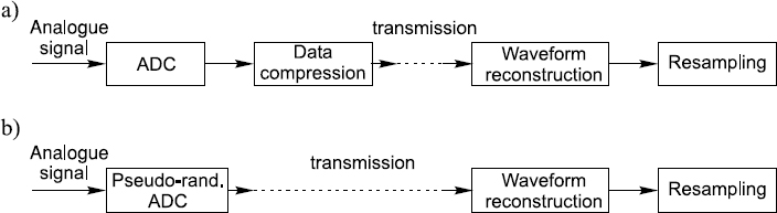
Figure 20.7 Typical difference between the (a) traditional and (b) suggested data compression/decompression schemes

The advantage of the considered pseudo-randomized data compression approach over the conventionally used data compression techniques is illustrated in Figure 20.7(b). The functional block for data compression is not included in the second scheme. It is not needed as data in the second case are actually presented in a compressed form at the output of the digitizer. Nothing special has to be done to compress the acquired data. Therefore it is evident that designs of the data acquisition subsystems exploiting this approach to data compression could be much simpler with reduced power consumption. The full computational burden in this case is placed on the functional block performing data decompression. For that, the waveform of the original signal usually has to be reconstructed. Once that is accomplished, this waveform could be represented by its equidistant sample values taken at a sufficiently high sampling rate to meet the requirement of the sampling theorem.

The embedded systems if they are built according to the scheme given in Figure 20.1 would support this data compression and reconstruction scheme. When they are used for dealing with analog signals, the data representing them are compressed at the stage of signal digitizing. In cases where these data are immediately processed, the computer performs the processing as required. If the given data have to be converted into a digital periodic signal sample value sequence, the computer performs data decompression and the signal waveform is reconstructed for that.

The computer of a particular embedded system apparently can reconstruct signal waveforms either by processing the digital signal taken from the output of the pseudo-randomized ADC included into the structure of this embedded system or by processing some other external digital signal encoded in a similar way. Figure 20.8 illustrates a few versions of the digital signals represented in various forms. The basic digital signal taken off the digitizer output is a sequence of the input signal sample values obtained at nonuniformly spaced time instants {t_k}. Both the numerical value and the sampling instant need to be given for each signal sample.

Figure 20.8 Various digital representations of the (a, b) compressed and (c) distorted data

This information can be encoded in various ways. Firstly, this kind of digital signal could be and often is presented in the form shown in Figure 20.8(a). In these cases, the digital time intervals (t_k+1 – t_k) between the sample values x_k+1 and x_k are equal to the time intervals between the respective sampling time instants. They are equal to some quantity of the smallest sampling time digits δ. The time diagram of a typical digital output signal of the pseudo-randomized ADC looks like this.

Figure 20.8(b) illustrates the second possible approach to the compressed data representation. It is shown that the signal sample values {x_k} and the respective sampling instants {t_k} could also be given by two periodic sequences of numerical values. However, it is much better to sample signals at precisely predetermined time instants and to use this sampling instant information for a reconstruction of the respective signal waveform. This approach should be used whenever possible. Then the compressed signal is simply a periodic sequence of the signal sample values and the information of the sampling process nonuniformity is kept in a memory as shown in Figure 20.1.

The third variety of the digital signals that could be processed by the considered embedded systems is given in Figure 20.8(c). It is a periodic signal with randomly skipped values. This type of signal has to be processed when a periodically sampled signal is distorted by some faults in functioning of the respective system. A typical task that has to be resolved is the reconstruction of the distorted and excluded signal sample values rather than decompression of some compressed data block. However, the waveform of the original signal apparently also needs to be restored in this case and when this reconstructed waveform is obtained there are no problems in reconstruction of the missing sample values.

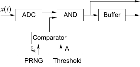
Figure 20.9 Block diagram of a device performing data compression by pseudo-random decimation of the digital signal present at the ADC output

20.4.2 Data Compression for One-Dimensional Signals

The basic advantage of the considered data compression/reconstruction approach is the extreme simplicity of the compression. Actually no special data processing functions need to be performed to compress data in this case. Indeed, to compress the data representing, for instance, one-dimensional signals given as periodic sequences of their sample values, the sample value sequences simply have to be pseudo-randomly decimated, with the remaining sample values packed and transmitted or stored as shorter periodic digital signals having a reduced number of discrete values. Forming of the compressed data blocks could be carried out using the scheme given in Figure 20.9.

Data representing the input signal are given as a uniform digital signal at the ADC output. The simple logic circuitry of this scheme dictates which of the signal sample values x_k are passed to the output and which are excluded. The PRNG is used for generation of pseudo-random numbers ξ_k within the range (0, 1). The AND gate is opened when the pseudo-random number ξ_k exceeds the threshold A. The signal sample values taken at these time instants are included in the output signal, all other sample values being omitted. Thus the signal at the output of the AND gate is periodic with pseudo-randomly skipped sample values. The threshold level A defines the probability of a signal sample value being missing. This signal representing the compressed data could be transmitted in this form with zeroes replacing the excluded sample values or the sample values could be stored in a buffer memory and then transmitted as a shorter periodic sequence.

Evidently this decimation of the signal sample values is performed for data compression in a way predetermined by the design of the PRNG and its synchronization to the signal. If the same type of properly synchronized PRNG is used at reconstruction of the compressed data, it is easy to replace the missing sample values by zeroes. Once that is done, any of the algorithms considered in Section 20.2 could be used for recovery of the original signal or, in other words, for decompression of data. The PRNG, of course, could be replaced by a memory containing a code prescribing the time instances at which the signal sample values should be eliminated.

Figure 20.10 illustrates a signal reconstructed from compressed data. The signal given in Figure 20.10(a) was reconstructed by using the SECOEX algorithm. The next signal shown in Figure 20.10(b) was reconstructed on the basis of the iterative reconstruction algorithm adapted to the pattern of the missing sample values. To obtain data for this demonstration under well-controlled conditions, a periodically sampled (sampling frequency 44.1 KS/s, 16-bit quantizing) signal, specifically recorded music, was used. These data were compressed three times in the described way and then reconstructed. The reconstructed sample values can be compared with the waveform of the original signal.

This example is given to show how data representing a signal could be compressed in a very simple way and then reconstructed. Although these data compression techniques can be used universally, they were actually developed for applications based on processing and transmission of RF and microwave signals.

20.4.3 Data Compression for Two-Dimensional Signals

Various techniques are used for compression of data representing twodimensional images. Typically they are relatively complicated. Therefore it is tempting to use the data compression approach described above for compressing this kind of two-dimensional data. A particular image of ‘Lena’, given in Figure 20.11(a), was reconstructed from data compressed four times. The compressed image with 75 % of pixels missing is shown in Figure 20.11(b). The restored image is given in Figure 20.11(c). The reconstruction was again based on the iterative reconstruction algorithm adapted to the pattern of the missing pixels.

The advantage of this approach to image compression is again in the extreme simplicity of the data compression procedure. Reconstruction of the images encoded in this way is computationally burdensome. However, the reconstruction quality is relatively good.

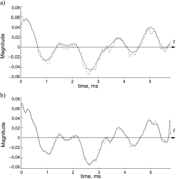
Figure 20.10 Signal waveform reconstructed (solid line) from data compressed three times. The original signal is given by dashed lines

20.4.4 Providing for Fault Tolerance

Fault-tolerant sensor systems represent yet another area in which application of the discussed embedded systems could turn out to be quite useful. The point is that the digital alias-free signal processing technology is well suited for performing under conditions when data are presented in a nonuniform way, which is exactly what is needed for reconstruction of data damaged as a result of system faults. Therefore application of this technology for the development of sensor signal processing systems tolerant to faulty signal sample values or to sensor failures is well worth considering.

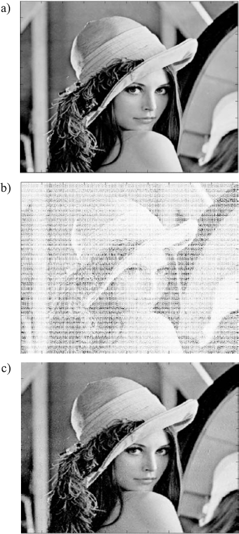
Figure 20.11 Illustration of two-dimensional data compressed four times and reconstruction of the respective image: (a) original image; (b) compressed image with 75% of the pixels taken out; (c) reconstructed image

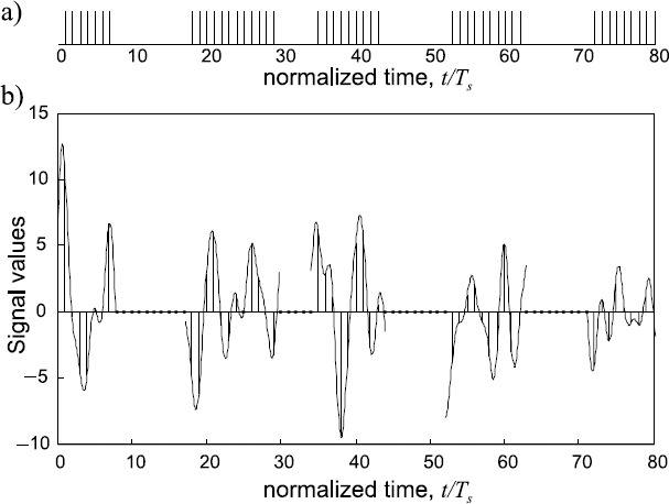
Figure 20.12 Illustration of a signal waveform distorted by faults

To demonstrate the potential of the algorithms discussed above for reconstruction of signals heavily distorted by fault bursts, a typical case of signal distortion by faults was simulated and the obtained results follow. It was assumed that as a digital sensor signal is corrupted by a powerful interference and many of the signal sample values are completely distorted they had to be taken out of this signal at time instants indicated in Figure 20.12(a) by zeroes. The signal waveform distorted by these fault bursts is shown in Figure 20.12(b).

The iterative signal reconstruction algorithm adapted to the specific fault sequence was used for recovery of the original signal. A zoomed segment of the reconstructed signal sample value sequence is given in Figure 20.13. It can be seen that the quality of the distorted signal reconstruction in this case is good as the sample values of the reconstructed signal overlap the original signal. As expected, the algorithms for reconstruction of signals from their nonuniform sample value sequences adapted to the sampling nonuniformities could be successfully used also for recovery of signals distorted by system faults.

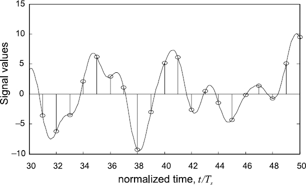
Figure 20.13 Segment (zoomed) of the reconstructed signal sample value sequence overlapping the waveform of the original signal

Note that while the approach to data compression–signal reconstruction described above is applicable for a wide variety of signals, the achievable reconstruction quality to a certain extent depends on spectra of them. To achieve good signal reconstruction adaptability to specific sampling irregularities, it should be possible to decompose the respective signals into their components and the frequencies of these components should be estimated with sufficiently high resolution and precision. That can usually be done but there might be problems.

20.5 Reducing the Quantity of Sensors in Large-aperture Arrays

The subject of high-performance complexity-reduced array signal processing is rather complicated and is actually beyond the scope of this book. Therefore only a few points on this subject are considered here, simply to draw attention to the fact that the discussed digital alias-free signal processing technology is quite competitive and has a high application potential in this area.

As explained in Chapter 17, pseudo-randomization of the distances between sensors in arrays helps in the suppression of the aliasing effect and under certain conditions might lead to a significant reduction in the number of sensors in arrays. However, to succeed, it is crucial to use appropriate nonuniform signal processing techniques for handling array signal processing, both in the time and spatial domains. While it is relatively easy to achieve suppression of spatial aliasing, there are problems with obtaining sufficiently precise estimates of the spatial spectrum not corrupted by noise related to the fuzzy aliasing effect. Figure 17.9 illustrates this fact. To achieve better results, special anti-aliasing array signal processing techniques and tools have to be used to take into account the cross-interference between components of nonuniformly sampled spatial signals. Although the required systems for processing spatial signals could be built in various ways, the development and use of application-specific embedded systems adaptable to the pattern of sensor positions in the array seems to be the best approach. The feasibility of the sensor quantity reduction achieved by such adaptation is confirmed by the results of computer simulations given below.

20.5.1 Adapting Signal Processing to Pseudo-random Positions of Sensors

As soon as the sensors are placed in an array nonuniformly, the spatial signals taken off this array strongly depend on the pattern of the sensor coordinates in the array. In particular, the basis functions for spatial spectrum analysis under these conditions become nonorthogonal, which leads to cross-interference between spatial signal components. The impact of this cross-interference is observed as background noise corrupting the results of spatial spectrum analysis and beamforming. This noise depends both on the irregularities of sensor positions in the array and on the received or transmitted signal.

The impact of cross-interference due to non-uniformities of sensor positions in the array could be characterized by cross-interference coefficients defined in a way similar to the definition (15.9). Specifically, these coefficients characterizing the cross-interference between the spatial signal components might be introduced as follows:

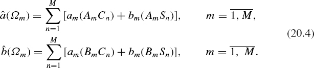
These coefficients are actually the weights of the errors introduced into the spatial signal in-phase component (or the quadrature component) at frequency Ω_n by nonuniform distancing of sensors. These errors corrupt the estimation of a Fourier coefficient a_m (or b_m) at spatial frequency Ω_m and therefore the coefficients (20.4) describe the interference between spatial frequency components of the array signal. Their definition is similar to the definition of the cross-interference coefficients (18.6) derived in Chapter 18 for the temporal spectrum analysis. In the case of the spatial spectrum analysis they are given as

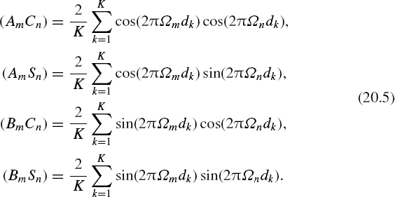
Another set of cross-interference coefficients, specifically coefficients A_nC_m, B_nC_m, A_nS_m and B_nS_m, characterize interference acting in the inverse direction from the spatial signal component Ω_m to the component Ω_n. It follows from (20.5) that

Thus the cross-interference effect, impacting spatial spectrum analysis in the case where sensors in the array are placed nonuniformly, is reflected by the following matrix of the cross-interference coefficients:

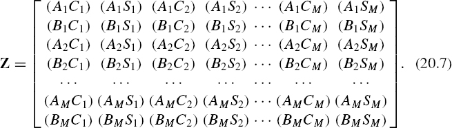
This matrix of the cross-interference coefficients is an essential characteristic of the arrays of sensors with pseudo-random distances between them. Once the pattern of sensors in the array is known, all coefficients of matrix Z, as well as of the matrix inv(Z), can be calculated. This means that when a signal is sampled in accordance with such a predetermined nonuniform sampling point process, an equation system similar to (18.19) could be solved, which adapts the estimation of the array signal parameters to the specific positions of the sensors in the array. That significantly reduces the impact of cross-interference between the estimates of the spatial spectrum parameters caused by pseudo-randomization of the array.

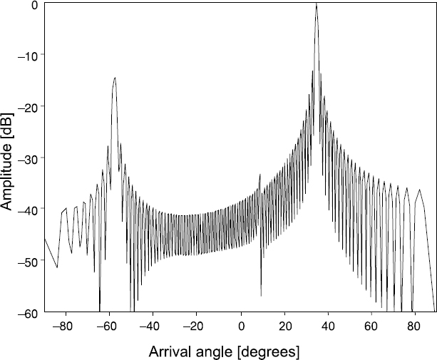
Figure 20.14 Estimated spatial spectrum of the array signal taken off the array of 128 equidistantly spaced sensors

This extension of the positive experience accumulated in the area of temporal signal processing for enhancement of array signal processing in the spatial domain seems to be quite successful. It is demonstrated by the following computer simulations. The spatial spectrum analysis of an array signal, containing three components with arrival angles and amplitudes Θ = 34.75° (0 dB), Θ = 8.96° (−42 dB) and = −57.37° (−15 dB), is simulated. Figure 20.14 illustrates the results of such an analysis obtained in the case where the array consists of 128 equidistantly placed sensors. To reduce the number of sensors in the array with the same aperture, the distances between the sensors need to be irregular otherwise there will be spatial aliasing. The results of the spatial spectrum analysis of the array signal formed by a nonuniform array containing a four times smaller amount of sensors (only 32) are given in Figure 20.15.

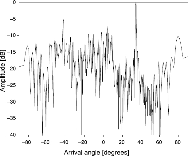
Figure 20.15 Results of the spatial DFT in the case where there are 32 nonuniformly placed sensors in the array

A comparison of the spectrograms given in Figures 20.14 and 20.15 leads to the conclusion that pseudo-randomization of the sensor array design alone does not lead to an acceptable array performance. To achieve better results, the spatial spectrum analysis has to be adapted to the specific irregularities of the sensor positions in the array, as explained above. Then the spectrograms are considerably less corrupted by background noise and are obtained in a significantly wider dynamic range. Figure 20.16 illustrates such adapting of spatial signal processing to the specific nonuniform pattern of the sensor locations in an array.

It can be seen from the obtained and displayed spectrograms in Figure 20.16 that deliberate randomization of sensor array designs does indeed make it possible to reduce the number of sensors in the arrays of the same aperture significantly. However, to benefit from this approach, it is crucial to use effective spatial signal processing techniques well matched to the specifics of this kind of array. The point is that the techniques used for adapting spatial signal processing to the irregularities of the sensor positions in arrays meet these requirements. They are capable of improving the performance of this type of sensor array significantly and therefore application of them makes it possible to reduce the number of sensors in the array.

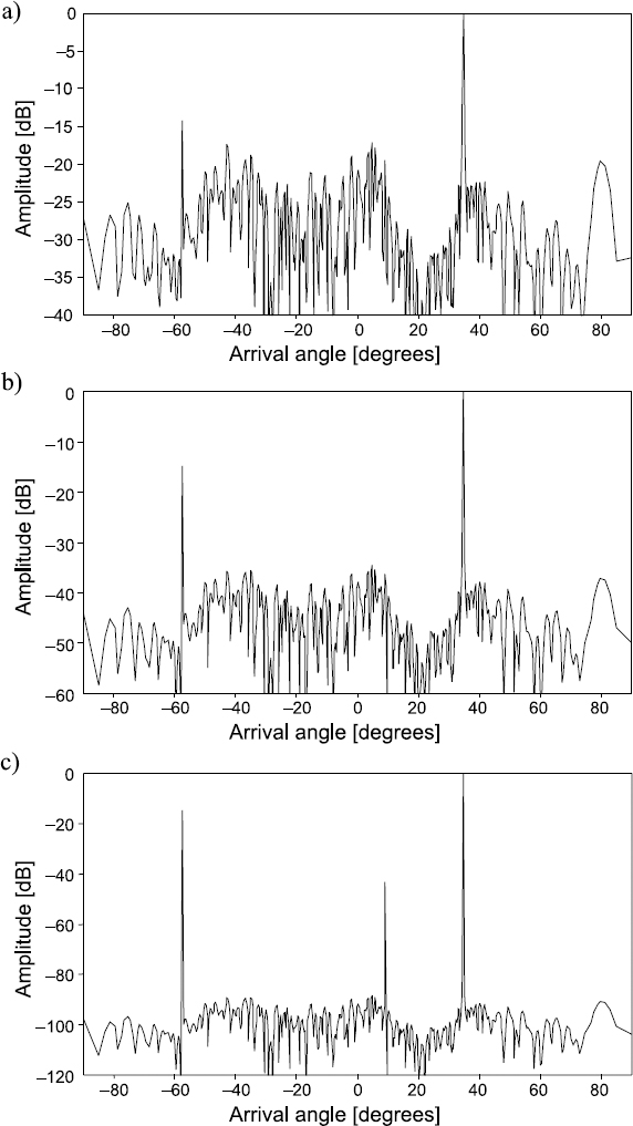
Figure 20.16 Spatial spectrum of a signal taken off an array of 32 pseudo-randomly spaced sensors obtained by adapting the spatial spectrum analysis to the nonuniformity of the sensor positions in the array: (a) after the second iteration; (b) after the fifth iteration; (c) after the tenth iteration

The achievable complexity reduction of this kind of irregular sensor array depends on the specific conditions of their applications. For instance, the array complexity and array signal processing time often needs to be traded-off. Nevertheless, it should be possible to reduce the number of sensors in arrays substantially in this way. As the research results so far obtained show, it is feasible to reduce in many cases the number of sensors in one-dimensional arrays from 4 to 5 times and from 16 to 25 times in two-dimensional arrays. It is evident that appropriate embedded systems for array signal processing, adapted to the irregularities of the respective sensor arrays, are needed and have to be used for that.

Bibliography

Allay, N. and Tarczynski, A. (2005) Direct digital recovery of modulated signals from their nonuniformly distributed samples. In Colloque International, TELECOM'2005 and 4 èmes Journées Fnanco-Maghré'bines des Micro-ondes it leurs Applications (JFMMA), INPT, Rabat, Moroc, March, pp. 535–8.

Artjuhs, J. and Bilinskis, I. (2006) Method and apparatus for alias suppressed digitizing of high frequency analog signals. EP 1 330 036 B1, European Patent Specification, Bulletin 2006/26, 28.06.2006.

Artyukh, Yu., Bilinskis, I., Greitans, M. and Vedin, V. (1997) Signal digitizing and recording in the DASPLab System. In Proceedings of the 1997 International Workshop on Sampling Theory and Application, Aveiro, Portugal, June 1997, pp. 357–60.

Artyukh, Yu., Bilinskis, I. and Vedin, V. (1999) Hardware core of the family of digital RF signal PC-based analyzers. In Proceedings of the 1999 International Workshop on Sampling Theory and Application, Loen, Norway, 11–14 August 1999, pp. 177–9.

Artyukh, J., Bilinskis, I., Boole, E., Rybakov, A. and Vedin, V. (2005) Wideband RF signal digititising for high purity spectral analysis. In Proceedings of the International Workshop on Spectral Methods and Multirate Signal Processing (SMMSP 2005), Riga, Latvia, 20–22 June 2005, pp. 123–8.

Bilinskis, I. and Artjuhs, J. (2006) Method and apparatus for alias suppressed digitizing of high frequency analog signals. United States Patent US 7,046,183 B2, 16 May 2006.

Bilinskis, I. and Cain, G. (1996) Digital alias-free signal processing in the GHz frequency range. In Digest of IEE Colloquium on Advanced Signal Processing for Microwave Applications, 29 November 1996.

Bilinskis, I. and Cain, G. (1996) Digital alias-free signal processing tolerance to data and sensor faults. In IEE Colloquium on Intelligent Sensors, Leicester, 1996.

Bilinskis, I. and Mikelsons, A. (1990) Application of randomized or irregular sampling as an anti-aliasing technique. In Signal Processing, V: Theories and Application. Amsterdam: Elsevier Science Publishers, pp. 505–8.

Bilinskis, I. and Rybakov, A. (2006) Iterative spectrum analysis of nonuniformly undersampled wideband signals. Electronics and Electrical Engineering, 4(68), 5–8.

Brannon, B. (1996) Wide-dynamic-range A/D converters pave the way for wideband digital-radio receivers. In EDN, 7 November 1996, pp. 187–205.

Brannon, B. Overcoming converter nonlinearities with dither. Analog Devices, AN-410, Application Note.

Harrington, R.F. (1961) Sidelobe reduction by nonuniform element spacing. IRE Trans. Antennas Propag., AP-9(2), 187–92.

Laakso, T.I., Murphy, N.P. and Tarczynski, A. (1996) Reconstruction of nonuniformly sampled signals using polynomial filtering. In Proceedings of the IEEE Nordic Signal Processing Symposium (NORSIG'96), Vol. 1, Helsinki, 24–27 September 1996, pp. 61–4.

Laakso, T.I., Tarczynski, A., Murphy, N.P. and Välimäki, V. (2000) Polynomial filtering approach to reconstruction and noise reduction of nonuniformly sampled signals. Signal Processing, 80(4), April, 567–75.

Lo, Y.T. (1964) Mathematical theory of antenna arrays with randomly spaced elements. IEEE Trans. Antennas Propag., AP-12, 257–68.

Lo, Y.T. and Simcoe, R.J. (1967) An experiment on antenna arrays with randomly spaced elements. IEEE Trans. Antennas Propag., AP-15, 231–5.

Marvasti, F. (2001) Nonuniform Sampling, Theory and Practice. New York: Kluwer Academic/Plenum Publishers.

Mednieks, I. and Mikelsons, A. (1990) Estimation of true components of wide-band quasi period signals. In Signal Processing, V: Theories and Application. Amsterdam: Elsevier Science Publishers, pp. 233–6.

Mikelsons, A. (1994) Alias-free spectral estimation of signals with components of arbitrary frequencies. In Adaptive Methods and Emergent Techniques for Signal Processing and Communications, Ljubljana, Slovenia, April 1994, pp. 105–8.

Mikelsons, A. and Greitans, M. (1996) Fault detection based on spectral estimation of nonuniformly sampled signals. In IEE Colloquium on Intelligent Sensors.

Tarczynski, A. (1997) Sensitivity of signal reconstruction. IEEE Signal Processing Letters, 4(7), July, pp. 192–4.

Tarczynski, A. (2002) Signal reconstruction from finite sets of arbitrarily distributed samples. In Proceedings of the 8th Biennial Baltic Electronics Conference (BEC2002), Tallinn, Estonia, 6–9 October 2002, pp. 233–6.

Tarczynski, A., Allay, N. and Qu, D. (2003) Reconstruction of nonuniformly sampled periodic signals. In 2003 International Workshop on Sampling Theory and Applications (SAMPTA'03), Strobl, Austria, 26–29 May 2003, pp. 94–9.

Tarczynski, A. and Cain, G.D. (1997) Reliability of signal reconstruction from finite sets of samples. In 1997 Workshop on Sampling Theory and Applications (SAMPTA'97), Vol. 1, Aveiro, 16–19 June 1997, pp. 181–6.

Tarczynski, A. and Qu, D. (2006) Reliability of signal reconstruction from arbitrarily distributed noisy samples. WSEAS Trans. on Signal Processing, 2(7), July, 925–32.

Tarczynski, A. and Qu, D. (2006) Quality assessment of reconstructing signals from arbitrarily distributed samples. In Proceedings of 10th International Conference on Systems, Vouliagmeni, Athens, Greece, 10–12 July 2006, pp. 7–13.