
CHAPTER 11
Organizing data
Search is an unsolved problem. We have a good 90 to 95% of the solution, but there is a lot to go in the remaining 10%.
Marissa Mayer, President and CEO of Yahoo!
Los Angeles Times interview (2008)
IN this age of “big data,” we take search algorithms for granted. Without web search sites that are able to sift through billions of pages in a fraction of a second, the web would be practically useless. Similarly, large data repositories, such as those maintained by the U.S. Geological Survey (USGS) and the National Institutes of Health (NIH), would be useless without the ability to search for specific information. Even the operating systems on our personal computers now supply integrated search capabilities to help us navigate our increasingly large collections of files.
To enable fast access to these sets of data, it must be organized in some way. A method for organizing data is known as a data structure. Hidden data structures in the implementations of the list and dictionary abstract data types enable their methods to access and modify their contents quickly. (The data structure behind a dictionary was briefly explained in Box 8.2.) In this chapter, we will explore one of the simplest ways to organize data—maintaining it in a sorted list—and the benefits this can provide. We will begin by developing a significantly faster search algorithm that can take advantage of knowing that the data is sorted. Then we will design three algorithms to sort data in a list, effectively creating a sorted list data structure. If you continue to study computer science, you can look forward to seeing many more sophisticated data structures in the future that enable a wide variety of efficient algorithms.
11.1 BINARY SEARCH
The spelling checkers that are built into most word processing programs work by searching through a list of English words, seeking a match. If the word is found, it is considered to be spelled correctly. Otherwise, it is assumed to be a misspelling. These word lists usually contain about a quarter million entries. If the words in the list are in no particular order, then we have no choice but to search through it one item at a time from the beginning, until either we happen to find the word we seek or we reach the end. We previously encountered this algorithm, called a linear search (or sequential search) because it searches in a linear fashion from beginning to end, and has linear time complexity.
Now let’s consider the improvements we can make if the word list has been sorted in alphabetical order, as they always are. At the very least, if we use a linear search on a sorted list, we know that we can abandon the search if we reach a word that is alphabetically after the word we seek. But we can do even better. Think about how we would search a physical, bound dictionary for the word “espresso.” Since “E” is in the first half of the alphabet, we might begin by opening the book to a point about 1/4 of the way through. Suppose that, upon doing so, we find ourselves on a page containing words beginning with the letter “G.” We would then flip backwards several pages, perhaps finding ourselves on a page on which the last word is “eagle.” Next, we would flip a few pages forward, and so on, continuing to hone in on “espresso” until we find it.
Reflection 11.1 Can we apply this idea to searching in a sorted list of values?
We can search a list in a similar way, except that we usually do not know much about the distribution of the list’s contents, so it is hard to make that first guess about where to start. In this case, the best strategy is to start in the middle. After comparing the item we seek to the middle item, we continue on the half of the list that must contain the item. Because we are effectively dividing the list into two halves each time, this algorithm is called binary search.
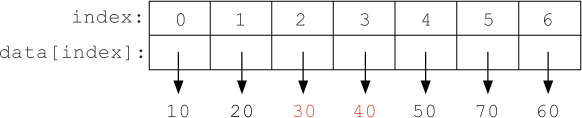
For example, suppose we wanted to search for the number 70 in the following sorted list of numbers. (We will use numbers instead of words in our example to save space.)
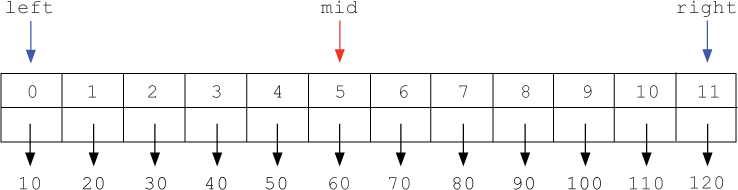
As we hone in on our target, we will update two variables named left and right to keep track of the first and last indices of the sublist that we are still considering.
A database is a structured file (or set of files) that contains a large amount of searchable data. The most common type of database, called a relational database, consists of some number of tables. Each row in a table represents one piece of data. Every row has a unique key that can be used to search for that row. For example, the tables below represent a small portion of the earthquake data that we worked with in Section 8.4.

The table on the left contains information about individual earthquakes, each of which is identified with a QuakeID that acts as its key. The last column contains a two-letter network code that identifies the preferred source of information about that earthquake. The table on the right contains the names associated with each two-letter code. The two-letter codes also act as the keys for this table.
Relational databases are queried using a programming language called SQL. A simple SQL query looks like this:
select Mag from Earthquakes where QuakeID = 'nc72076101'
This query is asking for the magnitude (Mag), from the Earthquakes table, of the earthquake with QuakeID nc72076101. The response to this query would be the value 1.8. Searching a table quickly for a particular key value is facilitated by an index. An index is data structure that maps key values to rows in a table (similar to a Python dictionary). The key values in the index can be maintained in sorted order so that any key value, and hence any row, can be found quickly using a binary search. (Database indices are more commonly maintained in practice in a hash table or a specialized data structure called a B-tree.)
In addition, we will maintain a variable named mid that is assigned to the index of the middle value of this sublist. (When there are two middle values, we choose the leftmost one.) In each step, we will compare the target item to the item at index mid. If the target is equal to this middle item, we return mid. Otherwise, we either set right to be mid - 1 (to hone in on the left sublist) or we set left to be mid + 1 (to hone in on the right sublist).
In the list above, we start by comparing the item at index mid (60) to our target item (70). Then, because 70 > 60, we decide to narrow our search to the second half of the list. To do this, we assign left to mid + 1, which is the index of the item immediately after the middle item. In this case, we assign left to 5 + 1 = 6, as shown below.

Then we update mid to be the index of the middle item in this sublist between left and right, in this case, 8. Next, since 70 is less than the new middle value, 90, we discard the second half of the sublist by assigning right to mid - 1, in this case, 8 - 1 = 7, as shown below.

Then we update mid to be 6, the index of the “middle” item in this short sublist. Finally, since the item at index mid is the one we seek, we return the value of mid.
Reflection 11.2 What would have happened if we were looking for a non-existent number like 72 instead?
If we were looking for 72 instead of 70, all of the steps up to this point would have been the same, except that when we looked at the middle item in the last step, it would not have been equal to our target. Therefore, picking up from where we left off, we would notice that 72 is greater than our middle item 70, so we update left to be the index after mid, as shown below.

Now, since left and right are both equal to 7, mid must be assigned to 7 as well. Then, since 72 is less than the middle item, 80, we continue to blindly follow the algorithm by assigning right to be one less than mid.
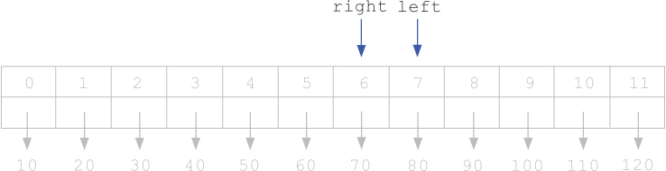
At this point, since right is to the left of left (i.e., left > right), the sublist framed by left and right is empty! Therefore, 72 must not be in the list, and we return –1.
This description of the binary search algorithm can be translated into a Python function in a very straightforward way:
def binarySearch(keys, target):
    """Find the index of target in a sorted list of keys.

    Parameters:
        keys: a list of key values
        target: a value for which to search

    Return value:
        the index of an occurrence of target in keys
    """

    n = len(keys)
    left = 0
    right = n - 1
    while left <= right:
        mid = (left + right) // 2
        if target < keys[mid]:
            right = mid - 1
        elif target > keys[mid]:
            left = mid + 1
        else:
            return mid
    return -1
Notice that we have named our list parameter keys (instead of the usual data) because, in real database applications (see Box 11.1), we typically try to match a target value to a particular feature of a data item, rather than to the entire data item. This particular feature is known as a key value. For example, in searching a phone directory, if we enter “Cumberbatch” in the search field, we are not looking for a directory entry (the data item) in which the entire contents contain only the word “Cumberbatch.” Instead, we are looking for a directory entry in which just the last name (the key value) matches Cumberbatch. When the search term is found, we return the entire directory entry that corresponds to this key value. In our function, we return the index at which the key value was found which, if we had data associated with the key, might provide us with enough information to find it in an associated data structure. We will look at an example of this in Section 11.2.
The binarySearch function begins by initializing left and right to the first and last indices in the list. Then, while left <= right, we compute the new value of mid and compare keys[mid] to the target we seek. If they are equal, we simply return the value of mid. Otherwise, we adjust left or right to hone in on target. If we get to the point where left > right, the loop ends and we return –1, having not found target.
Reflection 11.3 Write a main function that calls binarySearch with the list that we used in our example. Search for 70 and 72.
Reflection 11.4 Insert a statement in the binarySearch function, after mid is assigned its value, that prints the values of left, right, and mid. Then search for more target values. Do you see why mid is assigned to the printed values?
Efficiency of iterative binary search
How much better is binary search than linear search? When we analyzed the linear search in Section 6.7, we counted the worst case number of comparisons between the target and a list item, so let’s perform the same analysis for binary search. Since the binary search contains a while loop, we will need to think more carefully this time about when the worst case happens.
Reflection 11.5 Under what circumstances will the binary search algorithm perform the most comparisons between the target and a list item?
In the worst case, the while loop will iterate all the way until left > right. Therefore, the worst case number of item comparisons will be necessary when the item we seek is not found in the list. Let’s start by thinking about the worst case number of item comparisons for some small lists. First, suppose we have a list with length n = 4. In the worst case, we first look at the item in the middle of this list, and then are faced with searching a sublist with length 2. Next, we look at the middle item of this sublist and, upon not finding the item, search a sublist of length 1. After one final comparison to this single item, the algorithm will return –1. So we needed a total of 3 comparisons for a list of length 4.
Reflection 11.6 Now what happens if we double the size of the list to n = 8?
After we compare the middle item in a list with length n = 8 to our target, we are left with a sublist with length 4. We already know that a list with length 4 requires 3 comparisons in the worst case, so a list with length 8 must require 3+1 = 4 comparisons in the worst case. Similarly, a list with length 16 must require only one more comparison than a list with length 8, for a total of 5. And so on. This pattern is summarized in Table 11.1. Notice that a list with over a billion items requires at most 31 comparisons!
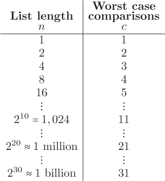
Table 11.1 The worst case number of comparisons for a binary search on lists with increasing lengths.
Reflection 11.7 Do you see the pattern in Table 11.1? For list of length n, how many comparisons are necessary in the worst case?
In each row of the table, the length of the list (n) is 2 raised to the power of 1 less than the number of comparisons (c), or
n = 2c–1.
Therefore, for a list of size n, the binary search requires
c = log2 n + 1
comparisons in the worst case. So binary search is a logarithmic-time algorithm. Since the time complexity of linear search is proportional to n, this means that linear search is exponentially slower than binary search.
This is a degree of speed-up that is only possible through algorithmic refinement; a faster computer simply cannot have this kind of impact. Figure 11.1 shows a comparison of actual running times of both search algorithms on some small lists. The time required by binary search is barely discernible as the red line parallel to the x-axis. But the real power of binary search becomes evident on very long lists. As suggested by Table 11.1, a binary search takes almost no time at all, even on huge lists, whereas a linear search, which must potentially examine every item, can take a very long time.

A spelling checker
Now let’s apply our binary search to the spelling checker problem with which we started this section. We can write a program that reads an alphabetized word list, and then allows someone to repeatedly enter a word to see if it is spelled correctly (i.e., is present in the list of words). A list of English words can be found on computers running Mac OS X or Linux in the file /usr/share/dict/words, or one can be downloaded from the book web site. This list is already sorted if you consider an upper case letter to be equivalent to its lower case counterpart. (For example, “academy” directly precedes “Acadia” in this file.) However, as we saw in Chapter 6, Python considers upper case letters to come before lower case letters, so we actually still need to sort the list to have it match Python’s definition of “sorted.” For now, we can use the sort method; in the coming sections, we will develop our own sorting algorithms. The following function implements our spelling checker.
def spellcheck():
    """Repeatedly ask for a word to spell-check and print the result.

    Parameters: none

    Return value: None
    """

    dictFile = open('/usr/share/dict/words', 'r', encoding = 'utf-8')
    wordList = [ ]

    for word in dictFile:
        wordList.append(word[:-1])
    dictFile.close()
    wordList.sort()

    word = input('Enter a word to spell-check (q to quit): ')
    while word != 'q':
        index = binarySearch(wordList, word)
        if index != -1:
            print(word, 'is spelled correctly.')
        else:
            print(word, 'is not spelled correctly.')
        print()
        word = input('Enter a word to spell-check (q to quit): ')
The function begins by opening the word list file and reading each word (one word per line) into a list. Since each line ends with a newline character, we slice it off before adding the word to the list. After all of the words have been read, we sort the list. The following while loop repeatedly prompts for a word until the letter q is entered. Notice that we ask for a word before the while loop to initialize the value of word, and then again at the bottom of the loop to set up for the next iteration. In each iteration, we call the binary search function to check if the word is contained in the list. If the word was found (index != -1), we state that it is spelled correctly. Otherwise, we state that it is not spelled correctly.
Reflection 11.8 Combine this function with the binarySearch function together in a program. Run the program to try it out.
Recursive binary search
You may have noticed that the binary search algorithm displays a high degree of self-similarity. In each step, the problem is reduced to solving a subproblem involving half of the original list. In particular, the problem of searching for an item between indices left and right is reduced to the subproblem of searching between left and mid - 1, or the subproblem of searching between mid + 1 and right. Therefore, binary search is a natural candidate for a recursive algorithm.
Like the recursive linear search from Section 10.4, this function will need two base cases. In the first base case, when the list is empty (left > right), we return -1. In the second base case, keys[mid] == item, so we return mid. If neither of these cases holds, we solve one of the two subproblems recursively. If the item we are searching for is less than the middle item, we recursively call the binary search with the right argument set to mid - 1. Or, if the item we are searching for is greater than the middle item, we recursively call the binary search with the left argument set to mid + 1.
def binarySearch(keys, target, left, right):
    """Recursively find the index of target in a sorted list of keys.

    Parameters:
        keys: a list of key values
        target: a value for which to search

    Return value:
        the index of an occurrence of target in keys
    """

    if left > right:              # base case 1: not found
        return -1
    mid = (left + right) // 2
    if target == keys[mid]:       # base case 2: found
        return mid
    if target < keys[mid]:        # recursive cases
        return binarySearch(keys, target, left, mid - 1)  # 1st half
    return binarySearch(keys, target, mid + 1, right)     # 2nd half
Reflection 11.9 Repeat Reflections 11.3 and 11.4 with the recursive binary search function. Does the recursive version “look at” the same values of mid?
Efficiency of recursive binary search
Like the iterative binary search, this algorithm also has logarithmic time complexity. But, as with the recursive linear search, we have to derive this result differently using a recurrence relation. Again, let the function T(n) denote the maximum (worst case) number of comparisons between the target and a list item in a binary search when the length of the list is n. In the function above, there are two such comparisons before reaching a recursive function call. As we did in Section 10.4, we will simply represent the number of comparisons before each recursive call with the constant c. When n = 0, we reach a base case with no recursive calls, so T(0) = c.
Reflection 11.10 How many more comparisons are there in a recursive call to binarySearch?
Since each recursive call divides the size of the list under consideration by (about) half, the size of the list we are passing into each recursive call is (about) n/2. Therefore, the number of comparisons in each recursive call must be T(n/2). The total number of comparisons is then
T(n) = T (n/2) + c.
Now we can use the same substitution method that we used with recursive linear search to arrive at a closed form expression in terms of n. First, since T(n) = T(n/2) + c, we can substitute T(n) with T(n/2) + c:

Figure 11.2 An illustration of how to derive a closed form for the recurrence relation T(n) = T(n/2) + c.

Now we need to replace T(n/2) with something. Notice that T(n/2) is just T(n) with n/2 substituted for n. Therefore, using the definition of T(n) above,
T (n/2) = T (n/2/2) + c = T (n/4) + c.
Similarly,
T (n/4) = T (n/4/2) + c = T (n/8) + c
and
T (n/8) = T (n/8/2) + c = T (n/16) + c.
This sequence of substitutions is illustrated in Figure 11.2. Notice that the denominator under the n at each step is a power of 2 whose exponent is the multiplier in front of the accumulated c’s at that step. In other words, for each denominator 2i, the accumulated value on the right is i · c. When we finally reach T(1) = T(n/n), the denominator has become n = 2log2 n, so i = log2 n and the total on the right must be (log2 n)c. Finally, we know that T(0) = c, so the total number of comparisons is
T(n) = (log2 n + 2) c.
Therefore, as expected, the recursive binary search is a logarithmic-time algorithm.
Exercises
11.1.1. How would you modify each of the binary search functions in this section so that, when a target is not found, the function also prints the values in keys that would be on either side of the target if it were in the list?
11.1.2. Write a function that takes a file name as a parameter and returns the number of misspelled words in the file. To check the spelling of each word, use binary search to locate it in a list of words, as we did above. (Hint: use the strip string method to remove extraneous punctuation.)
11.1.3. Write a function that takes three parameters—minLength, maxLength, and step—and produces a plot like Figure 11.1 comparing the worst case running times of binary search and linear search on lists with length minLength, minLength + step, minLength + 2 * step, ..., maxLength. Use a slice of the list derived from list(range(maxLength)) as the sorted list for each length. To produce the worst case behavior of each algorithm, search for an item that is not in the list (e.g., –1).
11.1.4. The function below plays a guessing game against the pseudorandom number generator. What is the worst case number of guesses necessary for the function to win the game for any value of n, where n is a power of 2? Explain your answer.
import random

def guessingGame(n):
    secret = random.randrange(1, n + 1)
    left = 1
    right = n
    guessCount = 1
    guess = (left + right) // 2
    while guess != secret:
        if guess > secret:
            right = guess - 1
        else:
            left = guess + 1
        guessCount = guessCount + 1
        guess = (left + right) // 2
    return guessCount
11.2 SELECTION SORT
Sorting is a well-studied problem, and a wide variety of sorting algorithms have been designed, including the one used by the familiar sort method of the list class. We will develop and compare three other common algorithms, named selection sort, insertion sort, and merge sort.
Reflection 11.11 Before you read further, think about how you would sort a list of data items (names, numbers, books, socks, etc.) in some desired order. Write down your algorithm informally.
The selection sort algorithm is so called because, in each step, it selects the next smallest value in the list and places it in its proper sorted position, by swapping it with whatever is currently there. For example, consider the list of numbers [50, 30, 40, 20, 10, 70, 60]. To sort this list in ascending order, the selection sort algorithm first finds the smallest number, 10. We want to place 10 in the first position in the list, so we swap it with the number that is currently in that position, 50, resulting in the modified list
[10, 30, 40, 20, 50, 70, 60]
Next, we find the second smallest number, 20, and swap it with the number in the second position, 30:
[10, 20, 40, 30, 50, 70, 60]
Then we find the third smallest number, 30, and swap it with the number in the third position, 40:
[10, 20, 30, 40, 50, 70, 60]
Next, we find the fourth smallest number, 40. But since 40 is already in the fourth position, no swap is necessary. This process continues until we reach the end of the list.
Reflection 11.12 Work through the remaining steps in the selection sort algorithm. What numbers are swapped in each step?
Implementing selection sort
Now let’s look at how we can implement this algorithm, using a more detailed representation of this list which, as usual, we will name data:
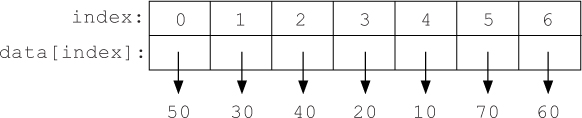
To begin, we want to search for the smallest value in the list, and swap it with the value at index 0. We have already seen how to accomplish key parts of this step. First, writing a function
swap(data, i, j)
to swap two values in a list was the objective of Exercise 8.2.5. In this swap function, i and j are the indices of the two values in the list data that we want to swap. And on Page 354, we developed a function to find the minimum value in a list. The min function used the following algorithm:
minimum = data[0]
for item in data[1:]:
    if item < minimum:
        minimum = item
The variable named minimum is initialized to the first value in the list, and updated with smaller values as they are encountered in the list.
Reflection 11.13 Once we have the final value of minimum, can we implement the first step of the selection sort algorithm by swapping minimum with the value currently at index 0?
Unfortunately, it is not quite that easy. To swap the positions of two values in data, we need to know their indices rather than their values. Therefore, in our selection sort algorithm, we will need to substitute minimum with a reference to the index of the minimum value. Let’s call this new variable minIndex. This substitution results in the following alternative algorithm.
n = len(data)
minIndex = 0
for index in range(1, n):
    if data[index] < data[minIndex]:
        minIndex = index
Notice that this algorithm is really the same as the previous algorithm; we are just now referring to the minimum value indirectly through its index (data[minIndex]) instead of directly through the variable minimum. Once we have the index of the minimum value in minIndex, we can swap the minimum value with the value at index 0 by calling
if minIndex != 0:
    swap(data, 0, minIndex)
Reflection 11.14 Why do we check if minIndex != 0 before calling the swap function?
In our example list, these steps will find the smallest value, 10, at index 4, and then call swap(data, 0, 4). We first check if minIndex != 0 so we do not needlessly swap the value in position 0 with itself. This swap results in the following modified list:

In the next step, we need to do almost exactly the same thing, but for the second smallest value.
Reflection 11.15 How we do we find the second smallest value in the list?
Notice that, now that the smallest value is “out of the way” at the front of the list, the second smallest value in data must be the smallest value in data[1:]. Therefore, we can use exactly the same process as above, but on data[1:] instead. This requires only four small changes in the code, marked in red below.
minIndex = 1
for index in range(2, n):
    if data[index] < data[minIndex]:
        minIndex = index
if minIndex != 1:
    swap(data, 1, minIndex)
Instead of initializing minIndex to 0 and starting the for loop at 1, we initialize minIndex to 1 and start the for loop at 2. Then we swap the smallest value into position 1 instead of 0. In our example list, this will find the smallest value in data[1:], 20, at index 3. Then it will call swap(data, 1, 3), resulting in the following modified list:

Similarly, the next step is to find the index of the smallest value starting at index 2, and then swap it with the value in index 2:
minIndex = 2
for index in range(3, n):
    if data[index] < data[minIndex]:
        minIndex = index
if minIndex != 2:
    swap(data, 2, minIndex)
In our example list, this will find the smallest value in data[2:], 30, at index 3. Then it will call swap(data, 2, 3), resulting in:
We continue by repeating this sequence of steps, with increasing values of the numbers in red, until we reach the end of the list.
To implement this algorithm in a function that works for any list, we need to situate the repeated sequence of steps in a loop that iterates over the increasing values in red. We can do this by replacing the initial value of minIndex in red with a variable named start:
minIndex = start
for index in range(start + 1, n):
    if data[index] < data[minIndex]:
        minIndex = index
if minIndex != start:
    swap(data, start, minIndex)
Then we place these steps inside a for loop that has start take on all of the integers from 0 to n - 2:
 1 def selectionSort(data):
 2     """Sort a list of values in ascending order using the
 3        selection sort algorithm.
 4
 5     Parameter:
 6         data: a list of values
 7
 8     Return value: None
 9     """
10
11     n = len(data)
12     for start in range(n - 1):
13         minIndex = start
14         for index in range(start + 1, n):
15             if data[index] < data[minIndex]:
16                 minIndex = index
17         if minIndex != start:
18             swap(data, start, minIndex)
Reflection 11.16 In the outer for loop of the selectionSort function, why is the last value of start n - 2 instead of n - 1? Think about what steps would be executed if start were assigned the value n - 1.
Reflection 11.17 What would happen if we called selectionSort with the list ['dog', 'cat', 'monkey', 'zebra', 'platypus', 'armadillo']? Would it work? If so, in what order would the words be sorted?

Figure 11.3 A comparison of the execution times of selection sort and the list sort method on small randomly shuffled lists.
Because the comparison operators are defined for both numbers and strings, we can use our selectionSort function to sort either kind of data. For example, call selectionSort on each of the following lists, and then print the results. (Remember to incorporate the swap function from Exercise 8.2.5.)
numbers = [50, 30, 40, 20, 10, 70, 60]
animals = ['dog', 'cat', 'monkey', 'zebra', 'platypus', 'armadillo']
heights = [7.80, 6.42, 8.64, 7.83, 7.75, 8.99, 9.25, 8.95]
Efficiency of selection sort
Next, let’s look at the time complexity of the selection sort algorithm. We can derive the asymptotic time complexity by counting the number of times the most frequently executed elementary step executes. The most frequently executed step in the selectionSort function is the comparison in the if statement on line 15. Since line 15 is in the body of the inner for loop (on line 14) and this inner for loop iterates a different number of times for each value of start in the outer for loop (on line 12), we must ask how many times the inner for loop iterates for each value of start. When start is 0, the inner for loop on line 14 runs from 1 to n – 1, for a total of n – 1 iterations. So line 15 is also executed n – 1 times. Next, when start is 1, the inner for loop runs from 2 to n – 1, a total of n – 2 iterations, so line 15 is executed n – 2 times. With each new value of start, there is one less iteration of the inner for loop. Therefore, the total number of times that line 15 is executed is
(n – 1) + (n – 2) + (n – 3) + …
Where does this sum stop? To find out, we look at the last iteration of the outer for loop, when start is n - 2. In this case, the inner for loop runs from n - 1 to n - 1, for only one iteration. So the total number of steps is
(n – 1) + (n – 2) + (n – 3) + … + 3 + 2 + 1.
What is this sum equal to? You may recall that we have encountered this sum a few times before (see Box 4.2):
Ignoring the constant 1/2 in front of n2 and the low order term (1/2)n, we find that this expression is asymptotically proportional to n2; hence selection sort has quadratic time complexity.
Figure 11.3 shows the results of an experiment comparing the running time of selection sort to the sort method of the list class. (Exercise 11.3.4 asks you to replicate this experiment.) The parabolic blue curve in Figure 11.3 represents the quadratic time complexity of the selection sort algorithm. The red curve at the bottom of Figure 11.3 represents the running time of the sort method. Although this plot compares the algorithms on very small lists on which both algorithms are very fast, we see a marked difference in the growth rates of the execution times. We will see why the sort method is so much faster in Section 11.4.
Querying data
Suppose we want to write a program that allows someone to query the USGS earthquake data that we worked with in Section 8.4. Although we did not use IDs then, each earthquake was identified by a unique ID such as ak10811825. The first two characters identify the monitoring network (ak represents the Alaska Regional Network) and the last eight digits represent a unique code assigned by the network. So our program needs to search for a given ID, and then return the attributes associated with that ID, say the earthquake’s latitude, longitude, magnitude, and depth. The earthquake IDs will act as keys, on which we will perform our searches. This associated data is sometimes called satellite data because it revolves around the key.
To use the efficient binary search algorithm in our program, we need to first sort the data by its key values. When we read this data into memory, we can either read it into parallel lists, as we did in Section 8.4, or we can read it into a table (i.e., a list of lists), as we did in Section 9.1. In this section, we will modify our selection sort algorithm to handle the first option. We will leave the second option as an exercise.
First, we will read the data into two lists: a list of keys (i.e., earthquake IDs) and a list of tuples containing the satellite data. For example, the satellite data for one earthquake that occurred at 19.5223 latitude and -155.5753 longitude with magnitude 1.1 and depth 13.6 km will be stored in the tuple (19.5223, -155.5753, 1.1, 13.6). Let’s call these two lists ids and data, respectively. (We will leave writing the function to read the IDs and data into their respective lists as an exercise.) By design, these two lists are parallel in the sense that the satellite data in data[index] belongs to the earthquake with ID in ids[index]. When we sort the earthquakes by ID, we will need to make sure that the associations with the satellite data are maintained. In other words, if, during the sort of the list ids, we swap the values in ids[9] and ids[4], we also need to swap data[9] and data[4].
To do this with our existing selection sort algorithm is actually quite simple. We pass both lists into the selection sort function, but make all of our sorting decisions based entirely on a list of keys. Then, when we swap two values in keys, we also swap the values in the same positions in data. The modified function looks like this (with changes in red):
def selectionSort(keys, data):
    """Sort parallel lists of keys and data values in ascending
       order using the selection sort algorithm.

    Parameters:
        keys: a list of keys
        data: a list of data values corresponding to the keys

    Return value: None
    """

    n = len(keys)
    for start in range(n - 1):
        minIndex = start
        for index in range(start + 1, n):
            if keys[index] < keys[minIndex]:
                minIndex = index
        swap(keys, start, minIndex)
        swap(data, start, minIndex)
Once we have the sorted parallel lists ids and data, we can use binary search to retrieve the index of a particular ID in the list ids, and then use that index to retrieve the corresponding satellite data from the list data. The following function does this repeatedly with inputted earthquake IDs.
def queryQuakes(ids, data):
    key = input('Earthquake ID (q to quit): ')
    while key != 'q':
        index = binarySearch(ids, key, 0, len(ids) - 1)
        if index >= 0:
            print('Location: ' + str(data[index][:2]) + '
' +
                  'Magnitude: ' + str(data[index][3]) + '
' +
                  'Depth: ' + str(data[index][2]) + '
')
        else:
            print('An earthquake with that ID was not found.')
        key = input('Earthquake ID (q to quit): ')
A main function that ties all three pieces together looks like this:
def main():
    ids, data = readQuakes()    # left as an exercise
    selectionSort(ids, data)
    queryQuakes(ids, data)
Exercises
11.2.1. Can you find a list of length 5 that requires more comparisons (on line 15) than another list of length 5? In general, with lists of length n, is there a worst case list and a best case list with respect to comparisons? How many comparisons do the best case and worst case lists require?
11.2.2. Now consider the number of swaps. Can you find a list of length 5 that requires more swaps (on line 18) than another list of length 5? In general, with lists of length n, is there a worst case list and a best case list with respect to swaps? How many swaps do the best case and worst case lists require?
11.2.3. The inner for loop of the selection sort function can be eliminated by using two built-in Python functions instead:
def selectionSort2(data):
    n = len(data)
    for start in range(n - 1):
        minimum = min(data[start:])
        minIndex = start + data[start:].index(minimum)
        if minIndex != start:
            swap(data, start, minIndex)
Is this function more or less efficient than the selectionSort function we developed above? Explain.
11.2.4. Suppose we already have a list that is sorted in ascending order, and want to insert new values into it. Write a function that inserts an item into a sorted list, maintaining the sorted order, without re-sorting the list.
11.2.5. Write a function that reads earthquake IDs and earthquake satellite data, consisting of latitude, longitude, depth and magnitude, from the data file on the web at
http://earthquake.usgs.gov/earthquakes/feed/v1.0/summary/2.5_month.csv
and returns two parallel lists, as described on Page 559. The satellite data for each earthquake should be stored as a tuple of floating point values. Then use this function to complete a working version of the program whose main function is shown on Page 560. (Remember to incorporate the recursive binary search and the swap function from Exercise 8.2.5.) Look at the above URL in a web browser to find some earthquake IDs to search for or do the next exercise to have your program print a list of all of them.
11.2.6. Add to the queryQuakes function on Page 560 the option to print an alphabetical list of all earthquakes, in response to typing list for the earthquake ID. For example, the output should look something like this:
Earthquake ID (q to quit): ci37281696
Location: (33.4436667, -116.6743333)
Magnitude: 0.54
Depth: 13.69

Earthquake ID (q to quit): list
    ID             Location         Magnitude  Depth
----------  ----------------------  ---------  -----
ak11406701   (63.2397, -151.4564)         5.5    1.3
ak11406705   (58.9801, -152.9252)        69.2    2.3
ak11406708   (59.7555, -152.6543)        80.0    1.9
   ...

uw60913561   (41.8655, -119.6957)         0.2    2.4
uw60913616   (44.2917, -122.6705)         0.0    1.3

Earthquake ID (q to quit):
11.2.7. An alternative to storing the earthquake data in two parallel lists is to store it in one table (a list of lists or a list of tuples). For example, the beginning of a table containing the earthquakes shown in the previous exercise would look like this:
[['ak11406701', 63.2397, -151.4564, 5.5, 1.3],
 ['ak11406705', 58.9801, -152.9252, 69.2, 2.3],
 ...
]
Rewrite the readQuakes, selectionSort, binarySearch, and queryQuakes functions so that they work with the earthquake data stored in this way instead. Your functions should assume that the key value for each earthquake is in column 0. Combine your functions into a working program that is driven by the following main function:
def main():
    quakes = readQuakes()
    selectionSort(quakes)
    queryQuakes(quakes)
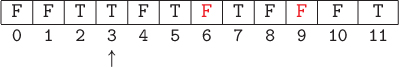
11.2.8. The Sieve of Eratosthenes is a simple algorithm for generating prime numbers that has a structure that is similar to the nested loop structure of selection sort. In this algorithm, we begin by initializing a list of n Boolean values named prime as follows. (In this case, n = 12.)
![]()
At the end of the algorithm, we want prime[index] to be False if index is not prime and True if index is prime. The algorithm continues by initializing a loop index variable to 2 (indicated by the arrow below) and then setting the list value of every multiple of 2 to be False.

Next, the loop index variable is incremented to 3 and, since prime[3] is True, the list value of every multiple of 3 is set to be False.
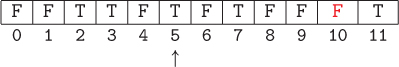
Next, the loop index variable is incremented to 4. Since prime[4] is False, we do not need to set any of its multiples to False, so we do not do anything.

This process continues with the loop index variable set to 5:
And so on. How far must we continue to increment index before we know we are done? Once we are done filling in the list, we can iterate over it one more time to build the list of prime numbers, in this case, [2, 3, 5, 7, 11]. Write a function that implements this algorithm to return a list of all prime numbers less than or equal to a parameter n.
11.3 INSERTION SORT
Our second sorting algorithm, named insertion sort, is familiar to anyone who has sorted a hand of playing cards. Working left to right through our hand, the insertion sort algorithm inserts each card into its proper place with respect to the previously arranged cards. For example, consider our previous list, arranged as a hand of cards:
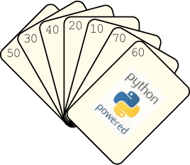
We start with the second card to the left, 30, and decide whether it should stay where it is or be inserted to the left of the first card. In this case, it should be inserted to the left of 50, resulting in the following slightly modified ordering:

Then we consider the third card from the left, 40. We see that 40 should be inserted between 30 and 50, resulting in the following order.

Next, we consider 20, and see that it should be inserted all the way to the left, before 30.

This process continues with 10, 70, and 60, at which time the hand is sorted.
Implementing insertion sort
To implement this algorithm, we need to repeatedly find the correct location to insert an item among the items to the left, assuming that the items to the left are already sorted. Let’s name the index of the item that we wish to insert insertIndex and the item itself itemToInsert. In other words, we assign
itemToInsert = data[insertIndex]
To illustrate, suppose that insertIndex is 4 (and itemToInsert is 10), as shown below:
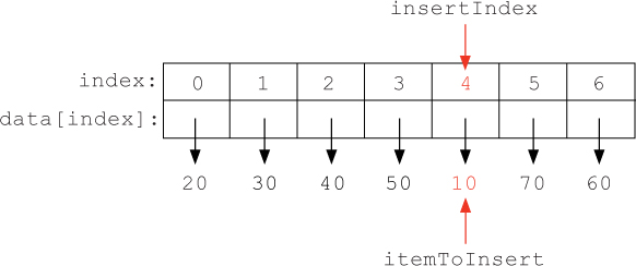
We need to compare itemToInsert to each of the items to the left, first at index insertIndex - 1, then at insertIndex - 2, insertIndex - 3, etc. When we come to an item that is less than or equal to itemToInsert or we reach the beginning of the list, we know that we have found the proper location for the item. This process can be expressed with a while loop:
itemToInsert = data[insertIndex]
index = insertIndex - 1
while index >= 0 and data[index] > itemToInsert:
    index = index - 1
The variable named index tracks which item we are currently comparing to itemToInsert. The value of index is decremented while it is still at least zero and the item at position index is still greater than itemToInsert. At the end of the loop, because the while condition has become false, either index has reached -1 or data[index] <= itemToInsert. In either case, we want to insert itemToInsert into position index + 1. In the example above, we would reach the beginning of the list, so we want to insert itemToInsert into position index + 1 = 0.
To actually insert itemToInsert in its correct position, we need to delete itemToInsert from its current position, and insert it into position index + 1.
data.pop(insertIndex)
data.insert(index + 1, itemToInsert)
In the insertion sort algorithm, we want to repeat this process for each value of insertIndex, starting at 1, so we enclose these steps in a for loop:
def insertionSort(data):
    """Sort a list of values in ascending order using the
       insertion sort algorithm.

     Parameter:
         data: a list of values

     Return value: None
     """

     n = len(data)
     for insertIndex in range(1, n):
         itemToInsert = data[insertIndex]
         index = insertIndex - 1
         while index >= 0 and data[index] > itemToInsert:
             index = index - 1
         data.pop(insertIndex)
         data.insert(index + 1, itemToInsert)
Although this function is correct, it performs more work than necessary. To see why, think about how the pop and insert methods must work, based on the picture of the list on Page 564. First, to delete (pop) itemToInsert, which is at position insertIndex, all of the items to the right, from position insertIndex + 1 to position n - 1, must be shifted one position to the left. Then, to insert itemToInsert into position index + 1, all of the items to the right, from position index + 2 to n - 1, must be shifted one position to the right. So the items from position insertIndex + 1 to position n - 1 are shifted twice, only to end up back where they started.
A more efficient technique would be to only shift those items that need to be shifted, and do so while we are already iterating over them. The following modified algorithm does just that.
 1 def insertionSort(data):
 2     """ (docstring omitted) """
 3
 4     n = len(data)
 5     for insertIndex in range(1, n):
 6         itemToInsert = data[insertIndex]
 7         index = insertIndex - 1
 8         while index >= 0 and data[index] > itemToInsert:
 9             data[index + 1] = data[index]
10             index = index - 1
11         data[index + 1] = itemToInsert
The red assignment statement in the for loop copies each item at position index one position to the right. Therefore, when we get to the end of the loop, position index + 1 is available to store itemToInsert.
Reflection 11.18 To get a better sense of how this works, carefully work through the steps with the three remaining items to be inserted in the illustration on Page 564.
Reflection 11.19 Write a main function that calls the insertionSort function to sort the list from the beginning of this section: [50, 30, 40, 20, 10, 70, 60].
Efficiency of insertion sort
Is the insertion sort algorithm any more efficient than selection sort? To discover its time complexity, we first need to identify the most frequently executed elementary step(s). In this case, these appear to be the two assignment statements on lines 9–10 in the body of the while loop. However, the most frequently executed step is actually the test of the while loop condition on line 8. To see why, notice that the condition of a while loop is always tested when the loop is first reached, and again after each iteration. Therefore, a while loop condition is always tested once more than the number of times the while loop body is executed. As we did with selection sort, we will count the number of times the while loop condition is tested for each value of the index in the outer for loop.
Unlike with selection sort, we need to think about the algorithm’s best case and worst case behavior since the number of iterations of the while loop depends on the values in the list being sorted.
Reflection 11.20 What are the minimum and maximum number of iterations executed by the while loop for a particular value of insertIndex?
In the best case, it is possible that the item immediately to the left of itemToInsert is less than itemToInsert, and therefore the condition is tested only once. Therefore, since there are n – 1 iterations of the outer for loop, there are only n – 1 steps total for the entire algorithm. So, in the best case, insertion sort is a linear-time algorithm.
On the other hand, in the worst case, itemToInsert may be the smallest item in the list and the while loop executes until index is less than 0. Since index is initialized to insertIndex - 1, the condition on line 8 is tested with index equal to insertIndex - 1, then insertIndex - 2, then insertIndex - 3, etc., until index is -1, at which time the while loop ends. In all, this is insertIndex + 1 iterations of the while loop. Therefore, when insertIndex is 1 in the outer for loop, there are two iterations of the while loop; when insertIndex is 2, there are three iterations of the while loop; when insertIndex is 3, there are four iterations of the while loop; etc. In total, there are 2 + 3 + 4 + … iterations of the while loop. As we did with selection sort, we need to figure out when this pattern ends. Since the last value of insertIndex is n - 1, the while loop condition is tested at most n times in the last iteration. So the total number of iterations of the while loop is
2 + 3 + 4 + … + (n – 1) + n.
Using the same trick we used with selection sort, we find that the total number of steps is
Ignoring the constants and lower order terms, this means that insertion sort is also a quadratic-time algorithm in the worst case.
So which case is more representative of the efficiency of insertion sort, the best case or the worst case? Computer scientists are virtually always interested in the worst case over the best case because the best case scenario for an algorithm is usually fairly specific and very unlikely to happen in practice. On the other hand, the worst case gives a robust upper limit on the performance of the algorithm. Although more challenging, it is also possible to find the average case complexity of some algorithms, assuming that all possible cases are equally likely to occur.
We can see from Figure 11.4 that the running time of insertion sort is almost identical to that of selection sort in practice. Since the best case and worst case of selection sort are the same, it appears that the worst case analysis of insertion sort is an accurate measure of performance on random lists. Both algorithms are still significantly slower than the built-in sort method, and this difference is even more apparent with longer lists. We will see why in the next section.
Exercises
11.3.1. Give a particular 10-element list that requires the worst case number of comparisons in an insertion sort. How many comparisons are necessary for this list?
11.3.2. Give a particular 10-element list that requires the best case number of comparisons in an insertion sort. How many comparisons are necessary for this list?
11.3.3. Write a function that compares the time required to sort a long list of English words using insertion sort to the time required by the sort method of the list class.
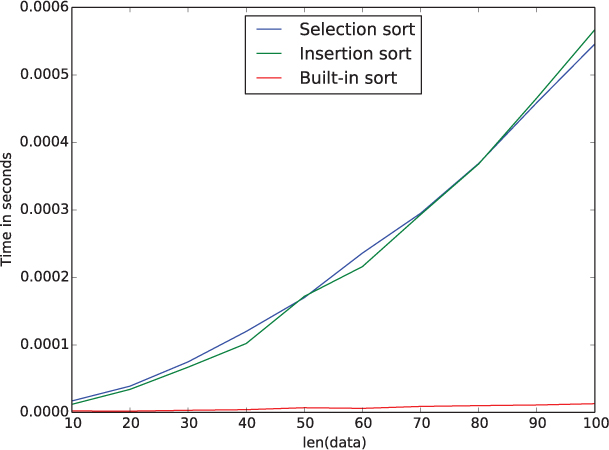
Figure 11.4 A comparison of the execution times of selection sort, insertion sort, and the list sort method on small randomly shuffled lists.
We can use the function time in the module of the same name to record the time required to execute each function. The time.time() function returns the number of seconds that have elapsed since January 1, 1970; so we can time a function by getting the current time before and after we call the function, and finding the difference.
As we saw in Section 11.1, a list of English words can be found on computers running Mac OS X or Linux in the file /usr/share/dict/words, or one can be downloaded from the book web site. This list is already sorted if you consider an upper case letter to be equivalent to its lower case counterpart. However, since Python considers upper case letters to come before lower case letters, the list is not sorted for our purposes.
Notes:
When you read in the list of words, remember that each line will end with a newline character. Be sure to remove that newline character before adding the word to your list.
Make a separate copy of the original list for each sorting algorithm. If you pass a list that has already been sorted by the
sortmethod to your insertion sort, you will not get a realistic time measurement because a sorted list is a best case scenario for insertion sort.
How many seconds did each sort require? (Be patient; insertion sort will take several minutes!) If you can be really patient, try timing selection sort as well.
sortPlot(minLength, maxLength, step)
that produces a plot like Figure 11.4 comparing the running times of insertion sort, selection sort, and the sort method of the list class on shuffled lists with length minLength, minLength + step, minLength + 2 * step, ..., maxLength. At the beginning of your function, produce a shuffled list with length maxLength with
data = list(range(maxLength))
random.shuffle(data)
Then time each function for each list length using a new, unsorted slice of this list.
11.3.5. A sorting algorithm is called stable if two items with the same value always appear in the sorted list in the same order as they appeared in the original list. Are selection sort and insertion sort stable sorts? Explain your answer in each case.
11.3.6. A third simple quadratic-time sort is called bubble sort because it repeatedly “bubbles” large items toward the end of the list by swapping each item repeatedly with its neighbor to the right if it is larger than this neighbor.
For example, consider the short list [3, 2, 4, 1]. In the first pass over the list, we compare pairs of items, starting from the left, and swap them if they are out of order. The illustration below depicts in red the items that are compared in the first pass, and the arrows depict which of those pairs are swapped because they are out of order.
![]()
At the end of the first pass, we know that the largest item (in blue) is in its correct location at the end of the list. We now repeat the process above, but stop before the last item.
![]()
After the second pass, we know that the two largest items (in blue) are in their correct locations. On this short list, we make just one more pass.
![]()
After n – 1 passes, we know that the last n – 1 items are in their correct locations. Therefore, the first item must be also, and we are done.
1 2 3 4
Write a function that implements this algorithm.
11.3.7. In the bubble sort algorithm, if no items are swapped during a pass over the list, the list must be in sorted order. So the bubble sort algorithm can be made somewhat more efficient by detecting when this happens, and returning early if it does. Write a function that implements this modified bubble sort algorithm. (Hint: replace the outer for loop with a while loop and introduce a Boolean variable that controls the while loop.)
11.3.8. Write a modified version of the insertion sort function that sorts two parallel lists named keys and data, based on the values in keys, like the parallel list version of selection sort on Page 559.
11.4 EFFICIENT SORTING
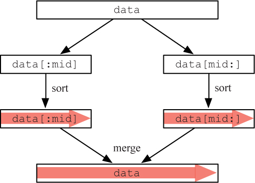
In the preceding sections, we developed two sorting algorithms, but discovered that they were both significantly less efficient than the built-in sort method. The algorithm behind the sort method is based on a recursive sorting algorithm called merge sort.1 The merge sort algorithm, like all recursive algorithms, constructs a solution from solutions to subproblems, in this case, sorts of smaller lists. As illustrated in Figure 11.5, the merge sort algorithm divides the original list into two halves, and then recursively sorts each of these halves. Once these halves are sorted, it merges them into the final sorted list.
Merge sort is a divide and conquer algorithm, like those you may recall from Section 10.5. Divide and conquer algorithms generally consist of three steps:
Divide the problem into two or more subproblems.
Conquer each subproblem recursively.
Combine the solutions to the subproblems into a solution for the original problem.
Reflection 11.21 Based on Figure 11.5, what are the divide, conquer, and combine steps in the merge sort algorithm?
The divide step of merge sort is very simple: just divide the list in half. The conquer step recursively calls the merge sort algorithm on the two halves. The combine step merges the two sorted halves into the final sorted list. This elegant algorithm can be implemented by the following function:

def mergeSort(data):
    """Recursively sort a list in place in ascending order,
       using the merge sort algorithm.

    Parameter:
        data: a list of values to sort

    Return value: None
    """

    n = len(data)
    if n > 1:
        mid = n // 2              # divide list in half
        left = data[:mid]
        right = data[mid:]
        mergeSort(left)           # recursively sort first half
        mergeSort(right)          # recursively sort second half
        merge(left, right, data)  # merge sorted halves into data
Reflection 11.22 Where is the base case in this function?
The base case in this function is implicit; when n <= 1, the function just returns because a list containing zero or one values is, of course, already sorted.
All that is left to flesh out mergeSort is to implement the merge function. Suppose we want to sort the list [60, 30, 50, 20, 10, 70, 40]. As illustrated in Figure 11.6, the merge sort algorithm first divides this list into the two sublists left = [60, 30, 50] and right = [20, 10, 70, 40]. After recursively sorting each of these lists, we have left = [30, 50, 60] and right = [10, 20, 40, 70]. Now we want to efficiently merge these two sorted lists into one final sorted list. We could, of course, concatenate the two lists and then call merge sort with them. But that would be far too much work; because the individual lists are sorted, we can do much better!

Figure 11.7 An illustration of the merge algorithm with the sublists left = [60, 30, 50] and right = [20, 10, 70, 40].
Since left and right are sorted, the first item in the merged list must be the minimum of the first item in left and the first item in right. So we place this minimum item into the first position in the merged list, and remove it from left or right. Then the next item in the merged list must again be one of the items at the front of left or right. This process continues until we run out of items in one of the lists.
This algorithm is illustrated in Figure 11.7. Rather than delete items from left and right as we append them to the merged list, we will simply maintain an index for each list to remember the next item to consider. The red arrows in Figure 11.7 represent these indices which, as shown in part (a), start at the left side of each list. In parts (a)–(b), we compare the two front items in left and right, append the minimum (10 from right) to the merged list, and advance the right index. In parts (b)–(c), we compare the first item in left to the second item in right, again append the minimum (20 from right) to the merged list, and advance the right index. This process continues until, after step (g), when the index in left exceeds the length of the list. At this point, we simply extend the merged list with whatever is left over in right, as shown in part (h).
Reflection 11.23 Work through steps (a) through (h) on your own to make sure you understand how the merge algorithm works.
This merge algorithm is implemented by the following function.
 1 def merge(left, right, merged):
 2     """Merge two sorted lists, named left and right, into
 3        one sorted list named merged.
 4
 5     Parameters:
 6         left: a sorted list
 7         right: another sorted list
 8         merged: the merged sorted list
 9
10     Return value: None
11     """
12
13     merged.clear()   # clear contents of merged
14     leftIndex = 0    # index in left
15     rightIndex = 0   # index in right
16
17     while leftIndex < len(left) and rightIndex < len(right):
18         if left[leftIndex] <= right[rightIndex]:
19             merged.append(left[leftIndex])    # left value is smaller
20             leftIndex = leftIndex + 1
21         else:
22             merged.append(right[rightIndex])  # right value is smaller
23             rightIndex = rightIndex + 1
24
25     if leftIndex >= len(left):             # items remaining in right
26         merged.extend(right[rightIndex:])
27     else:                                  # items remaining in left
28         merged.extend(left[leftIndex:])
The merge function begins by clearing out the contents of the merged list and initializing the indices for the left and right lists to zero. The while loop starting at line 17 constitutes the main part of the algorithm. While both indices still refer to items in their respective lists, we compare the items at the two indices and append the smallest to merged. When this loop finishes, we know that either leftIndex >= len(left) or rightIndex >= len(right). In the first case (lines 25–26), there are still items remaining in right to append to merged. In the second case (lines 27–28), there are still items remaining in left to append to merged.
Reflection 11.24 Write a program that uses the merge sort algorithm to sort the list in Figure 11.6.
Internal vs. external sorting
We have been assuming that the data that we want to sort is small enough to fit in a list in a computer’s memory. The selection and insertion sort algorithms must have the entire list in memory at once because they potentially pass over the entire list in each iteration of their outer loops. For this reason, they are called internal sorting algorithms.
But what if the data is larger than the few gigabytes that can fit in memory all at once? This is routinely the situation with real databases. In these cases, we need an external sorting algorithm, one that can sort a data set in secondary storage by just bringing pieces of it into memory at a time. The merge sort algorithm is just such an algorithm. In the merge function, each of the sorted halves could reside in a file on disk and just the current front item in each half can be read into memory at once. When the algorithm runs out of items in one of the sorted halves, it can simply read in some more. The merged list can also reside in a file on disk; when a new item is added to end of the merged result, it just needs to be written to the merged file after the previous item. Exercise 11.4.7 asks you to write a version of the merge function that merges two sorted files in this way.
Efficiency of merge sort
To discover the time complexity of merge sort, we need to set up a recurrence relation like the one we developed for the recursive binary search. We can again let T(n) represent the number of steps required by the algorithm with a list of length n. The mergeSort function consists of two recursive calls to mergeSort, each one with a list that is about half as long as the original. Like binary search, each of these recursive calls must require T(n/2) comparisons. But unlike binary search, there are two recursive calls instead of one. Therefore,
T(n) = 2T(n/2) + ?
where the question mark represents the number of steps in addition to the recursive calls, in particular to split data into left and right and to call the merge function.
Reflection 11.25 How many steps must be required to split the list into left and right?
Since every item in data is copied through slicing to one of the two lists, this must require about n steps.
Reflection 11.26 How many steps does the merge function require?
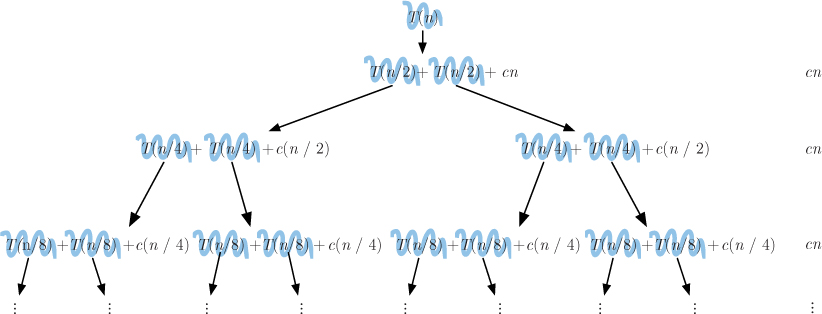
Figure 11.8 An illustration of how to derive a closed form for the recurrence relation T(n) = 2T(n/2) + cn.

Figure 11.9 A comparison of the execution times of selection sort and merge sort on small randomly shuffled lists.
Because either leftIndex or rightIndex is incremented in every iteration, the merge function iterates at most once for each item in the sorted list. So the total number of steps must be proportional to n. Therefore, the additional steps in the recurrence relation must also be proportional to n. Let’s call this number cn, where c is some constant. Then the final recurrence relation describing the number of steps in merge sort is
T(n) = 2T(n/2) + cn.
Finding a closed form for this recurrence is just slightly more complicated than it was for recursive binary search. Figure 11.8 illustrates the sequence of substitutions. Since there are two substitutions in each instance of the recurrence, the number of terms doubles in each level. But notice that the sum of the leftover values at each level is always equal to cn. As with the binary search recurrence, the size of the list (i.e., the argument of T) is divided in half with each level, so the number of levels is the same as it was with binary search, except that the base case with merge sort happens with n = 1 instead of n = 0. Looking back at Figure 11.2, we see that we reached n = 1 after log2 n + 1 levels. Therefore, the total number of steps must be
T(n) = (log2 n + 1) cn = cn log2 n + cn,
which is proportional to n log2 n asymptotically.
How much faster is this than the quadratic-time selection and insertion sorts? Figure 11.9 illustrates the difference by comparing the merge sort and selection sort functions on small randomly shuffled lists. The merge sort algorithm is much faster. Recall that the algorithm behind the built-in sort method is based on merge sort, which explains why it was so much faster than our previous sorts. Exercise 11.4.1 asks you to compare the algorithms on much longer lists as well.
Exercises
11.4.1. To keep things simple, assume that the selection sort algorithm requires exactly n2 steps and the merge sort algorithm requires exactly n log2 n steps. About how many times slower is selection sort than merge sort when n = 100? n = 1000? n = 1 million?
11.4.2. Repeat Exercise 11.3.3 with the merge sort algorithm. How does the time required by the merge sort algorithm compare to that of the insertion sort algorithm and the built-in sort method?
11.4.3. Add merge sort to the running time plot in Exercise 11.3.4. How does its time compare to the other sorts?
11.4.4. Our mergeSort function is a stable sort, meaning that two items with the same value always appear in the sorted list in the same order as they appeared in the original list. However, if we changed the <= operator in line 18 of the merge function to a < operator, it would no longer be stable. Explain why.
11.4.5. We have seen that binary search is exponentially faster than linear search in the worst case. But is it always worthwhile to use binary search over linear search?
The answer, as is commonly the case in the “real world”, is “it depends.” In this exercise, you will investigate this question. Suppose we have an unordered list of n items that we wish to search.
- If we use the linear search algorithm, what is the time complexity of this search?
- If we use the binary search algorithm, what is the time complexity of this search?
- If we perform n (where n is also the length of the list) individual searches of the list, what is the time complexity of the n searches together if we use the linear search algorithm?
- If we perform n individual searches with the binary search algorithm, what is the time complexity of the n searches together?
- What can you conclude about when it is best to use binary search vs. linear search?
11.4.6. Suppose we have a list of n keys that we anticipate needing to search k times. We have two options: either we sort the keys once and then perform all of the searches using a binary search algorithm or we forgo the sort and simply perform all of the searches using a linear search algorithm. Suppose the sorting algorithm requires exactly n2/2 steps, the binary search algorithm requires log2 n steps, and the linear search requires n steps. Assume each step takes the same amount of time.
- If the length of the list is n = 1024 and we perform k = 100 searches, which alternative is better?
- If the length of the list is n = 1024 and we perform k = 500 searches, which alternative is better?
- If the length of the list is n = 1024 and we perform k = 1000 searches, which alternative is better?
11.4.7. Write a function that merges two sorted files into one sorted file. Your function should take the names of the three files as parameters. Assume that all three files contain one string value per line. Your function should not use any lists, instead reading only one item at a time from each input file and writing one item at a time to the output file. In other words, at any particular time, there should be at most one item from each file assigned to any variable in your function. You will know when you have reached the end of one of the input files when a read function returns the empty string. There are two files on the book web site that you can use to test your function.
*11.5 TRACTABLE AND INTRACTABLE ALGORITHMS
The merge sort algorithm is much faster than the quadratic-time selection and insertion sort algorithms, but all of these algorithms are considered to be tractable, meaning that they can generally be expected to finish in a “reasonable” amount of time. We consider any algorithm with time complexity that is a polynomial function of n (e.g., n, n2, n5) to be tractable, while algorithms with time complexities that are exponential functions of n are intractable. An intractable algorithm is essentially useless with all but the smallest inputs; even if it is correct and will eventually finish, the answer will come long after anyone who needs it is dead and gone.

Table 11.2 A comparison of the approximate times required by algorithms with various time complexities on a computer capable of executing 1 billion steps per second.
To motivate this distinction, Table 11.2 shows the execution times of five algorithms with different time complexities, on a hypothetical computer capable of executing one billion operations per second. We can see that, for n up to 30, all five algorithms complete in about a second or less. However, when n = 50, we start to notice a dramatic difference: while the first four algorithms still execute very quickly, the exponential-time algorithm requires 13 days to complete. When n = 100, it requires 41 trillion years, about 3,000 times the age of the universe, to complete. And the differences only get more pronounced for larger values of n; the first four, tractable algorithms finish in a “reasonable” amount of time, even with input sizes of 1 billion,2 while the exponential-time algorithm requires an absurd amount of time. Notice that the difference between tractable and intractable algorithms holds no matter how fast our computers get; a computer that is one billion times faster than the one used in the table can only bring the exponential-time algorithm down to 10275 years from 10284 years when n = 1, 000!
The dramatic time differences in Table 11.2 also illustrate just how important efficient algorithms are. In fact, advances in algorithm efficiency are often considerably more impactful than faster hardware. Consider the impact of improving an algorithm from quadratic to linear time complexity. On an input with n equal to 1 million, we would see execution time improve from 16.7 minutes to 1/1000 of a second, a factor of one million! According to Moore’s Law (see Box 11.2), such an increase in hardware performance will not manifest itself for about 30 more years!
Moore’s Law is named after Gordon Moore, a co-founder of the Intel Corporation. In 1965, he predicted that the number of fundamental elements (transistors) on computer chips would double every year, a prediction he revised to every 2 years in 1975. It was later noted that this would imply that the performance of computers would double every 18 months. This prediction has turned out to be remarkably accurate, although it has started to slow down a bit as we run into the limitations of current technology. We have witnessed similar exponential increases in storage and network capacity, and the density of pixels in computer displays and digital camera sensors.
Consider the original Apple IIe computer, released in 1983. The Apple IIe used a popular microprocessor called the 6502, created by MOS Technology, which had 3,510 transistors with features as small as 8 µm and ran at a clock rate of 1 MHz. Current Apple Macintosh and Windows computers use Intel Core processors. The recent Intel Core i7 (Haswell) quad-core processor contains 1.4 billion transistors with features as small as 22 nm, running at a maximum clock rate of 3.5 GHz. In 30 years, the number of transistors has increased by a factor of almost 400,000, the transistors have become 350 times smaller, and the clock rate has increased by a factor of 3,500.
Hard problems
Unfortunately, there are many common, simply stated problems for which the only known algorithms have exponential time complexity. For example, suppose we have n tasks to complete, each with a time estimate, that we wish to delegate to two assistants as evenly as possible. In general, there is no known way to solve this problem that is any better than trying all possible ways to delegate the tasks and then choosing the best solution. This type of algorithm is known as a brute force or exhaustive search algorithm. For this problem, there are two possible ways to assign each task (to one of the two assistants), so there are
possible ways to assign the n tasks. Therefore, the brute force algorithm has exponential time complexity. Referring back to Table 11.2, we see that even if we only have n = 50 tasks, the brute force algorithm would be of no use to us.
It turns out that there are thousands of such problems, known as the NP-hard problems, that, on the surface, do not seem as if they should be intractable, but, as far as we know, they are. Even more interesting, no one has actually proven that they are intractable. See Box 11.3 if you would like to know more about this fascinating problem.
When we cannot solve a problem exactly, one common approach is to instead use a heuristic. A heuristic is a type of algorithm that does not necessarily give a correct answer, but tends to work well in practice. For example, a heuristic for the task delegation problem might assign the tasks in order, always assigning the next task to the assistant with the least to do so far. Although this will not necessarily give the best solution, it may be “good enough” in practice.
The P=NP problem is the most important unresolved question in computer science. Formally, the question involves the tractability of decision problems, problems with a “yes” or “no” answer. For example, the decision version of the task delegation problem would ask, “Is there is a task allocation that is within m minutes of being even?” Problems like the original task delegation problem that seek the value of an optimal solution are called optimization problems.
The “P” in “P=NP” represents the class of all tractable decision problems (for which algorithms with Polynomial time complexity are known). “NP” (short for “Nondeterministic Polynomial”) represents the class of all decision problems for which a candidate solution can be verified to be correct in polynomial time. For example, in the task delegation problem, a verifier would check whether a task delegation is within m minutes of being even. (This is a much easier problem!) Because any problem that can be solved in polynomial time must have a polynomial time verifier, we know that a problem in the class P is also contained in the class NP.
The NP-complete problems are the hardest problems in NP. (NP-hard problems are usually optimization versions of NP-complete problems.) “P=NP” refers to the question of whether all of the problems in NP are also in P or have polynomial time algorithms. Since so many brilliant people have worked on this problem for over 40 years, it is assumed that no polynomial-time algorithms exist for NP-hard problems.
11.6 SUMMARY
Sorting and searching are perhaps the most fundamental problems in computer science for good reason. We have seen how simply sorting a list can exponentially decrease the time it takes to search it, using the binary search algorithm. Since binary search is one of those algorithms that “naturally” exhibits self-similarity, we designed both iterative and recursive algorithms that implement the same idea. We also designed two basic sorting algorithms named selection sort and insertion sort. Each of these algorithms can sort a short list relatively quickly, but they are both very inefficient when it comes to larger lists. By comparison, the recursive merge sort algorithm is very fast. Merge sort has the added advantage of being an external sorting algorithm, meaning we can adapt it to sort very large data sets that cannot be brought into a computer’s memory all at once.
Although the selection and insertion sort algorithms are quite inefficient compared to merge sort, they are still tractable, meaning that they will finish in a “reasonable” amount of time. In fact, all algorithms with time complexities that are polynomial functions of their input sizes are considered to be tractable. On the other hand, exponential-time algorithms are called intractable because even when their input sizes are relatively small, they require eons to finish.
11.7 FURTHER DISCOVERY
This chapter’s epigraph is from an interview given by Marissa Mayer to the Los Angeles Times in 2008 [16].
The subjects of this chapter are fundamental topics in second-semester computer science courses, and there are many books available that cover them in more detail. A higher-level overview of some of the tricks used to make searching fast can be found in John MacCormick’s Nine Algorithms that Changed the Future [30].
11.8 PROJECTS
Project 11.1 Creating a searchable database
Write a program that allows for the interactive search of a data set, besides the earthquake data from Section 11.2, downloaded from the web or the book web site. It may be data that we have worked with elsewhere in this book or it may be a new data set. Your program, at a minimum, should behave like the program that we developed in Section 11.2. In particular, it should:
Read the data into a table or parallel lists.
Sort the data by an appropriate key value.
Interactively allow someone to query the data (by a key value). When a key value is found, the program should print the satellite data associated with that key. Use binary search to search for the key and return the results.
Project 11.2 Binary search trees
In this project, you will write a program that allows for the interactive search of a data set using an alternative data structure called a binary search tree (BST). Each key in a binary search tree resides in a node. Each node also contains references to a left child node and a right child node. The nodes are arranged so that the key of the left child of a node is less than or equal to the key of the node and the key of the right child is greater than the key of the node. For example, Figure 11.10 shows a binary search tree containing the numbers that we sorted in previous sections. The node at the top of the tree is called the tree’s root.
To insert a new item into a binary search tree, we start at the root. If the new item is less than or equal to the root, we next look at the left child. On the other hand, if the new item is greater than the root, we next look at the right child. Then we repeat this step on the next node, and continue until we arrive at a position without a node. Figure 11.11 illustrates how the value 35 would be inserted into the binary search tree in Figure 11.10. Starting at the root, since 35 < 50, we move to the left. Next, since 35 > 30, we next move to the right. Then, since 35 < 40, we move to the left. Since there is no node in this position, we create a new node with 35 and insert it there, as the left child of the node containing 40.
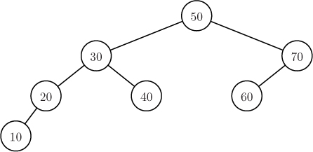
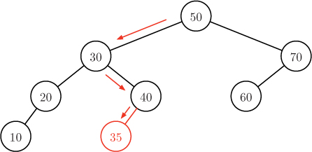
Question 11.2.1 How would the values 5, 25, 65, and 75 be inserted into the binary search tree in Figure 11.10?
Question 11.2.2 Does the order in which items are inserted affect what the tree looks like? After the four values in the previous question are inserted into the binary search tree, insert the value 67. Would the binary search tree be different if 67 were inserted before 65?
Searching a binary search tree follows the same process, except that we check whether the target value is equal to the key in each node that we visit. If it is, we return success. Otherwise, we move to the left or right, as we did above. If we eventually end up in a position without a node, we know that the target value was not found. For example, if we want to search for 20 in the binary search tree in Figure 11.10, we would start at the root and first move left because 20 < 50. Then we move left again because 20 < 30. Finally, we return success because we found our target. If we were searching for 25 instead, would have moved right when we arrived at node 20, but finding no node there, we would have returned failure.
Question 11.2.3 What nodes would be visited in searches for 10, 25, 55, and 60 in the binary search tree in Figure 11.10?
In Python, we can represent a node in a binary search tree with a three-item list. As illustrated below, the first item in the list is the key, the second item is a list representing the left child node, and the third item is a list representing the right child node.

The list above represents a single node with no left or right child. Or, equivalently, we can think of the two empty lists as representing “empty” left and right children. To insert a child, we simply insert into one of the empty lists the items representing the desired node. For example, to make 70 the right child of the node above, we would insert a new node containing 70 into the second list:
[50, [ ], [70, [ ], [ ]]]
To insert 60 as the left child of 70, we would insert a new node containing 60 into the first list in 70:
[50, [ ], [70, [60, [ ], [ ]], [ ]]]
The list above now represents the root and the two nodes to the right of the root in Figure 11.10. Notice that an entire binary search tree can be represented by its root node. The complete binary search tree in Figure 11.10 looks like this:
bst = [50, [30, [20, [10, [], []], []], [40, [], []]],
           [70, [60, [], []], []]]
Question 11.2.4 Parse the list above to understand how it represents the binary search tree in Figure 11.10.
This representation quickly becomes difficult to read. But, luckily, we will rely on our functions to read them instead of us.
Let’s now implement the insert and search algorithms we discussed earlier, using this list implementation. To make our code easier to read, we will define three constant values representing the indices of the key, left child, and right child in a node:
KEY = 0
LEFT = 1
RIGHT = 2
So if node is the name of a binary search tree node, then node[KEY] is the node’s key value, node[LEFT] is the node’s left child, and node[RIGHT] is the node’s right child.
The following function inserts a new node into a binary search tree:
def insert(root, key):
    """Insert a new key into the BST with the given root.

    Parameters:
        root: the list representing the BST
        key: the key value to insert

    Return value: None
    """

    current = root
    while current != [ ]:
        if key <= current[KEY]:
            current = current[LEFT]
        else:
            current = current[RIGHT]
    current.extend([key, [ ], [ ]])
The variable named current keeps track of where we are in the tree during the insertion process. The while loop proceeds to “move” current left or right until current reaches an empty node. At that point, the loop ends, and the algorithm inserts a new node containing key by inserting key and two empty lists into the empty list assigned to current. (Recall that the extend method effectively appends each item in its list argument to the end of the list.) To use this function to insert the value 35 into our binary search tree named bst above, as in Figure 11.11, we would call insert(bst, 35).
The function to search a binary search tree is very similar:
def search(root, key):
    """Search for a target key in the BST with the given root.

    Parameters:
        root: the list representing the BST
        key: the key value to search for

    Return value: a Boolean indicating whether key was found
    """

    current = root
    while current != [ ] and current[KEY] != key:
        if key < current[KEY]:
            current = current[LEFT]
        else:
            current = current[RIGHT]
    return current != [ ]
The only differences in the search function are (a) the loop now also ends if we find the desired key value in the node assigned to current, and (b) at the end of the loop, we return False (failure) if current ends at an empty node and True otherwise.
In this project, you will work with a data set of your choice, downloaded from the web or the book web site. It may be data that we have worked with elsewhere in this book or it may be a new data set. Your data must contain two or more attributes per entry, one of which will be an appropriate key value. The remaining attributes will constitute the satellite data associated with the entry.
Part 1: Extend the BST implementation
Extend the list representation of a node so that each node can store both a key and associated satellite data. Think about how your new design will affect the insert and search functions. Then modify these functions so that they work with your new representation.
With this extension, you are actually creating a new data structure that implements a dictionary abstract data type. The dictionary abstract data type in Python defines a way to insert (key, value) pairs and retrieve the value associated with a key using indexing. As explained in Box 8.2, Python dictionaries are usually implemented using a data structure called a hash table. In your extended binary search tree data structure, the insert function will insert a new (key, value) pair into the dictionary and the search function will return the value associated with key, if it is found, or None if it is not. We will revisit a dictionary implementation in Section 13.6.
Part 2: Read the data
Write a function that creates an empty binary search tree, reads your data from the web or a file, and then inserts each entry into the binary search tree.
Part 3: Allow queries
Write a function, like the queryQuakes function from Section 11.2, that allows someone to interactively query your data. The function should prompt for a key value, and then print the associated satellite data. To locate this data, search for the key in your binary search tree.
Question 11.2.5 Is searching a binary search tree as efficient as using the binary search algorithm to search in a sorted list? In what situations might a binary search tree not be as efficient? Explain your answers.
Write a main function that puts all of the pieces together to create a program that reads your data set and allows repeated queries of the data.
Part 4: Recursion
Every node in a binary search tree is the root of a subtree. In this way, binary search trees exhibit self-similarity. The subtrees rooted by a node’s left and right children are called the node’s left subtree and right subtree, respectively. Exploiting this self-similarity, we can think about inserting into (or searching) a binary search tree with root r as recursively solving one of two subproblems: inserting into the left subtree of r or inserting into the right subtree of r. Write recursive versions of the insert and search functions that use this self-similarity.
Part 5: Sorting
Once data is in a binary search tree, we have a lot of information about how it is ordered. We can use this structure to create a sorted list of the data. Notice that a sorted list of the keys in a binary search tree consists of a sorted list of the keys in the left subtree, followed by the root of the tree, followed by a sorted list of the keys in the right subtree. Using this insight, write a recursive function bstSort(root) that returns a sorted list of the keys in a binary search tree. Then use this function to add an option to your query function from Part 3 that prints the list of keys when requested.
Question 11.2.6 How efficient do you think this sorting algorithm is? How do you think it compares to the sorting algorithms we discussed in this chapter? (Remember to take into account the time it takes to insert the keys into the binary search tree.)
1The Python sorting algorithm, called Timsort, has elements of both merge sort and insertion sort. If you would like to learn more, go to http://bugs.python.org/file4451/timsort.txt
2Thirty-one years is admittedly a long time to wait, and no one would actually wait that long, but it is far shorter than 41 trillion years.