
CHAPTER 8
Data analysis
“Data! Data! Data!” he cried impatiently. “I can’t make bricks without clay.”
Sherlock Holmes
The Adventure of the Copper Beeches (1892)
IN Chapter 6, we designed algorithms to analyze and manipulate text, which is stored as a sequence of characters. In this chapter, we will design algorithms to process and learn from more general collections of data. The problems in this chapter involve earthquake measurements, SAT scores, isotope ratios, unemployment rates, meteorite locations, consumer demand, river flow, and more. Data sets such as these have become a (if not, the) vital component of many scientific, non-profit, and commercial ventures. Many of these now employ experts in data science and/or data mining who use advanced techniques to transform data into valuable information to guide the organization.
To solve these problems, we need an abstract data type (ADT) in which to store a collection of data. The simplest and most intuitive such abstraction is a list, which is simply a sequence of items. In previous chapters, we discovered how to generate Python list objects with the range function and how to accumulate lists of coordinates to visualize in plots. To solve the problems in this chapter, we will also grow and shrink lists, and modify and rearrange their contents, without having to worry about where or how they are stored in memory.
8.1 SUMMARIZING DATA
A list is represented as a sequence of items, separated by commas, and enclosed in square brackets ([ ]). Lists can contain any kind of data we want; for example:
>>> sales = [32, 42, 11, 15, 58, 44, 16]
>>> unemployment = [0.082, 0.092, 0.091, 0.063, 0.068, 0.052]
>>> votes = ['yea', 'yea', 'nay', 'yea', 'nay']
>>> points = [[2, 1], [12, 3], [6, 5], [3, 14]]
The first example is a list representing hundreds of daily sales, the second example is a list of the 2012 unemployment rates of the six largest metropolitan areas, and the third example is a list of votes of a five-member board. The last example is a list of (x, y) coordinates, each of which is represented by a two-element list. Although they usually do not in practice, lists can also contain items of different types:
>>> crazy = [15, 'gtaac', [1, 2, 3], max(4, 14)]
>>> crazy
[15, 'gtaac', [1, 2, 3], 14]
Since lists are sequences like strings, they can also be indexed and sliced. But now indices refer to list elements instead of characters and slices are sublists instead of substrings:
>>> sales[1]
42
>>> votes[:3]
['yea', 'yea', 'nay']
Now suppose that we are running a small business, and we need to get some basic descriptive statistics about last week’s daily sales, starting with the average (or mean) daily sales for the week. Recall from Section 1.2 that, to find the mean of a list of numbers, we need to first find their sum by iterating over the list. Iterating over the values in a list is essentially identical to iterating over the characters in a string, as illustrated below.
def mean(data):
    """Compute the mean of a list of numbers.

    Parameter:
        data: a list of numbers

    Return value: the mean of the numbers in data
    """

    sum = 0
    for item in data:
        sum = sum + item
    return sum / len(data)
In each iteration of the for loop, item is assigned the next value in the list named data, and then added to the running sum. After the loop, we divide the sum by the length of the list, which is retrieved with the same len function we used on strings.
Reflection 8.1 Does this work when the list is empty?
If data is the empty list ([ ]), then the value of len(data) is zero, resulting in a “division by zero” error in the return statement. We have several options to deal with this. First, we could just let the error happen. Second, if you read Section 7.2, we could use an assert statement to print an error message and abort. Third, we could detect this error with an if statement and return something that indicates that an error occurred. In this case, we will adopt the last option by returning None and indicating this possibility in the docstring.
 1 def mean(data):
 2     """Compute the mean of a non-empty list of numbers.
 3
 4     Parameter:
 5         data: a list of numbers
 6
 7     Return value: the mean of numbers in data or None if data is empty
 8     """
 9
10     if len(data) == 0:
11         return None
12
13     sum = 0
14     for item in data:
15         sum = sum + item
16     return sum / len(data)
This for loop is yet another example of an accumulator, and is virtually identical to the countLinks function that we developed in Section 4.1. To illustrate what is happening, suppose we call mean from the following main function.
def main():
    sales = [32, 42, 11, 15, 58, 44, 16]
    averageSales = mean(sales)
    print('Average daily sales were', averageSales)

main()
The call to mean(sales) above will effectively execute the following sequence of statements inside the mean function. The changing value of item assigned by the for loop is highlighted in red. The numbers on the left indicate which line in the mean function is being executed in each step.
14    sum = 0                     # sum is initialized
15    item = 32                   # for loop assigns 32 to item
16    sum = sum + item            # sum is assigned 0 + 32 = 32
15    item = 42                   # for loop assigns 42 to item

16    sum = sum + item            # sum is assigned 32 + 42 = 74
           ⋮
15    item = 16                   # for loop assigns 16 to item
16    sum = sum + item            # sum is assigned 202 + 16 = 218
17    return sum / len(data)      # returns 218 / 7 ≈ 31.14
Reflection 8.2 Fill in the missing steps above to see how the function arrives at a sum of 218.
The mean of a data set does not adequately describe it if there is a lot of variability in the data, i.e., if there is no “typical” value. In these cases, we need to accompany the mean with the variance, which is measure of how much the data varies from the mean. Computing the variance is left as Exercise 8.1.10.
Now let’s think about how to find the minimum and maximum sales in the list. Of course, it is easy for us to just look at a short list like the one above and pick out the minimum and maximum. But a computer does not have this ability. Therefore, as you think about these problems, it may be better to think about a very long list instead, one in which the minimum and maximum are not so obvious.
Reflection 8.3 Think about how you would write an algorithm to find the minimum value in a long list. (Similar to a running sum, keep track of the current minimum.)
As the hint suggests, we want to maintain the current minimum while we iterate over the list with a for loop. When we examine each item, we need to test whether it is smaller than the current minimum. If it is, we assign the current item to be the new minimum. The following function implements this algorithm.
def min(data):
    """Compute the minimum value in a non-empty list of numbers.

    Parameter:
        data: a list of numbers

    Return value: the minimum value in data or None if data is empty
    """

    if len(data) == 0:
        return None

    minimum = data[0]
    for item in data[1:]:
        if item < minimum:
            minimum = item
    return minimum
Before the loop, we initialize minimum to be the first value in the list, using indexing. Then we iterate over the slice of remaining values in the list. In each iteration, we compare the current value of item to minimum and, if item is smaller than minimum, update minimum to the value of item. At the end of the loop, minimum is assigned the smallest value in the list.
Reflection 8.4 If the list [32, 42, 11, 15, 58, 44, 16] is assigned to data, then what are the values of data[0] and data[1:]?
Let’s look at a small example of how this function works when we call it with the list containing only the first four numbers from the list above: [32, 42, 11, 15]. The function begins by assigning the value 32 to minimum. The first value of item is 42. Since 42 is not less than 32, minimum remains unchanged. In the next iteration of the loop, the third value in the list, 11, is assigned to item. In this case, since 11 is less than 32, the value of minimum is updated to 11. Finally, in the last iteration of the loop, item is assigned the value 15. Since 15 is greater than 11, minimum is unchanged. At the end, the function returns the final value of minimum, which is 11. A function to compute the maximum is very similar, so we leave it as an exercise.
Reflection 8.5 What would happen if we iterated over data instead of data[1:]? Would the function still work?
If we iterated over the entire list instead, the first comparison would be useless (because item and minimum would be the same) so it would be a little less efficient, but the function would still work fine.
Now what if we also wanted to know on which day of the week the minimum sales occurred? To answer this question, assuming we know how indices correspond to days of the week, we need to find the index of the minimum value in the list. As we learned in Chapter 6, we need to iterate over the indices in situations like this:
def minDay(data):
    """Compute the index of the minimum value in a non-empty list.

     Parameter:
         data: a list of numbers

     Return value: the index of the minimum value in data
                   or -1 if data is empty
     """

     if len(data) == 0:
         return -1

     minIndex = 0
     for index in range(1, len(data)):
         if data[index] < data[minIndex]:
             minIndex = index
     return minIndex
This function performs almost exactly the same algorithm as our previous min function, but now each value in the list is identified by data[index] instead of item and we remember the index of current minimum in the loop instead of the actual minimum value.
Reflection 8.6 How can we modify the minDay function to return a day of the week instead of an index, assuming the sales data starts on a Sunday.
One option would be to replace return minIndex with if/elif/else statements, like the following:
if minIndex == 0:
    return 'Sunday'
elif minIndex == 1:
    return 'Monday'
 ⋮
else:
    return 'Saturday'
But a more clever solution is to create a list of the days of the week that are in the same order as the sales data. Then we can simply use the value of minIndex as an index into this list to return the correct string.
days = ['Sunday', 'Monday', 'Tuesday', 'Wednesday', 'Thursday',
        'Friday', 'Saturday']
return days[minIndex]
There are many other descriptive statistics that we can use to summarize the contents of a list. The following exercises challenge you to implement some of them.
Exercises
8.1.1. Suppose a list is assigned to the variable name data. Show how you would
- print the length of
data - print the third element in
data - print the last element in
data - print the last three elements in
data - print the first four elements in
data - print the list consisting of the second, third, and fourth elements in
data
8.1.2. In the mean function, we returned None if data was empty. Show how to modify the following main function so that it properly tests for this possibility and prints an appropriate message.
def main():
    someData = getInputFromSomewhere()
    average = mean(someData)
    print('The mean value is', average)
8.1.3. Write a function
sumList(data)
that returns the sum of all of the numbers in the list data. For example, sumList([1, 2, 3]) should return 6.
8.1.4. Write a function
sumOdds(data)
that returns the sum of only the odd integers in the list data. For example, sumOdds([1, 2, 3]) should return 4.
8.1.5. Write a function
countOdds(data)
that returns the number of odd integers in the list data. For example, countOdds([1, 2, 3]) should return 2.
8.1.6. Write a function
multiples5(data)
that returns the number of multiples of 5 in a list of integers. For example, multiples5([5, 7, 2, 10]) should return 2.
8.1.7. Write a function
countNames(words)
that returns the number of capitalized names in the list of strings named words. For example, countNames(['Fili', 'Oin', 'Thorin', 'and', 'Bilbo', 'are', 'characters', 'in', 'a', 'book', 'by', 'Tolkien']) should return 5.
8.1.8. The percentile associated with a particular value in a data set is the number of values that are less than or equal to it, divided by the total number of values, times 100. Write a function
percentile(data, value)
that returns the percentile of value in the list named data.
meanSquares(data)
that returns the mean (average) of the squares of the numbers in a list named data.
variance(data)
that returns the variance of a list of numbers named data. The variance is defined to be the mean of the squares of the numbers in the list minus the square of the mean of the numbers in the list. In your implementation, call your function from Exercise 8.1.9 and the mean function from this section.
8.1.11. Write a function
max(data)
that returns the maximum value in the list of numbers named data. Do not use the built-in max function.
8.1.12. Write a function
shortest(words)
that returns the shortest string in a list of strings named words. In case of ties, return the first shortest string. For example, shortest(['spider', 'ant', 'beetle', 'bug'] should return the string 'ant'.
8.1.13. Write a function
span(data)
that returns the difference between the largest and smallest numbers in the list named data. Do not use the built-in min and max functions. (But you may use your own functions.) For example, span([9, 4, 2, 1, 7, 7, 3, 2]) should return 8.
maxIndex(data)
that returns the index of the maximum item in the list of numbers named data. Do not use the built-in max function.
8.1.15. Write a function
secondLargest(data)
that returns the second largest number in the list named data. Do not use the built-in max function. (But you may use your maxIndex function from Exercise 8.1.14.)
search(data, target)
that returns True if the target is in the list named data, and False otherwise. Do not use the in operator to test whether an item is in the list. For example, search(['Tris', 'Tobias', 'Caleb'], 'Tris') should return True, but search(['Tris', 'Tobias', 'Caleb'], 'Peter') should return False.
8.1.17. Write a function
search(data, target)
that returns the index of target if it is found in the list named data, and -1 otherwise. Do not use the in operator or the index method to test whether items are in the list. For example, search(['Tris', 'Tobias', 'Caleb'], 'Tris') should return 0, but search(['Tris', 'Tobias', 'Caleb'], 'Peter') should return -1.
8.1.18. Write a function
intersect(data1, data2)
that returns True if the two lists named data1 and data2 have any common elements, and False otherwise. (Hint: use your search function from Exercise 8.1.16.) For example, intersect(['Katniss', 'Peeta', 'Gale'], ['Foxface', 'Marvel', 'Glimmer']) should return False, but intersect(['Katniss', 'Peeta', 'Gale'], ['Gale', 'Haymitch', 'Katniss']) should return True.
8.1.19. Write a function
differ(data1, data2)
that returns the first index at which the two lists data1 and data2 differ. If the two lists are the same, your function should return -1. You may assume that the lists have the same length. For example, differ(['CS', 'rules', '!'], ['CS', 'totally', 'rules!']) should return the index 1.
8.1.20. A checksum is a digit added to the end of a sequence of data to detect error in the transmission of the data. (This is a generalization of parity from Exercise 6.1.11 and similar to Exercise 6.3.17.) Given a sequence of decimal digits, the simplest way to compute a checksum is to add all of the digits and then find the remainder modulo 10. For example, the checksum for the sequence 48673 is 8 because (4 + 8 + 6 + 7 + 3) mod 10 = 28 mod 10 = 8. When this sequence of digits is transmitted, the checksum digit will be appended to the end of the sequence and checked on the receiving end. Most numbers that we use on a daily basis, including credit card numbers and ISBN numbers, as well as data sent across the Internet, include checksum digits. (This particular checksum algorithm is not particularly good, so “real” checksum algorithms are a bit more complicated; see, for example, Exercise 8.1.21.)
- Write a function
checksum(data)
that computes the checksum digit for the list of integers nameddataand returns the list with the checksum digit added to the end. For example,checksum([4, 8, 6, 7, 3])should return the list[4, 8, 6, 7, 3, 8]. - Write a function
check(data)
that returns a Boolean value indicating whether the last integer indatais the correct checksum value. - Demonstrate a transmission (or typing) error that could occur in the sequence
[4, 8, 6, 7, 3, 8](the last digit is the checksum digit) that would not be detected by thecheckfunction.
8.1.21. The Luhn algorithm is the standard algorithm used to validate credit card numbers and protect against accidental errors. Read about the algorithm online, and then write a function
validateLuhn(number)
that returns True if the number if valid and False otherwise. The number parameter will be a list of digits. For example, to determine if the credit card number 4563 9601 2200 1999 is valid, one would call the function with the parameter [4, 5, 6, 3, 9, 6, 0, 1, 2, 2, 0, 0, 1, 9, 9, 9]. (Hint: use a for loop that iterates in reverse over the indices of the list.)
8.2 CREATING AND MODIFYING LISTS
We often want to create or modify data, rather than just summarize it. We have already seen some examples of this with the list accumulators that we have used to build lists of data to plot. In this section, we will revisit some of these instances, and then build upon them to demonstrate some of the nuts and bolts of working with data stored in lists. Several of the projects at the end of this chapter can be solved using these techniques.
List accumulators, redux
We first encountered lists in Section 4.1 in a slightly longer version of the following function.
import matplotlib.pyplot as pyplot

def pond(years):
    """ (docstring omitted) """

    population = 12000
    populationList = [population]
    for year in range(1, years + 1):
        population = 1.08 * population - 1500
        populationList.append(population)
    pyplot.plot(range(years + 1), populationList)
    pyplot.show()
    return population
In the first red statement, the list named populationList is initialized to the single-item list [12000]. In the second red statement, inside the loop, each new population value is appended to the list. Finally, the list is plotted with the pyplot.plot function.
We previously called this technique a list accumulator, due to its similarity to integer accumulators. List accumulators can be applied to a variety of problems. For example, consider the find function from Section 6.5. Suppose that, instead of returning only the index of the first instance of the target string, we wanted to return a list containing the indices of all the instances:
def find(text, target):
    """ (docstring omitted) """

     indexList = []
     for index in range(len(text) - len(target) + 1):
         if text[index:index + len(target)] == target:
             indexList.append(index)
     return indexList
In this function, just as in the pond function, we initialize the list before the loop, and append an index to the list inside the loop (wherever we find the target string). At the end of the function, we return the list of indices. The function call
find('Well done is better than well said.', 'ell')
would return the list [1, 26]. On the other hand, the function call
find('Well done is better than well said.', 'Franklin')
would return the empty list [] because the condition in the if statement is never true.
This list accumulator pattern is so common that there is a shorthand for it called a list comprehension. You can learn more about list comprehensions by reading the optional material at the end of this section, starting on Page 368.
Lists are mutable
We can modify an existing list with append because, unlike strings, lists are mutable. In other words, the components of a list can be changed. We can also change individual elements in a list. For example, if we need to change the second value in the list of unemployment rates, we can do so:
>>> unemployment = [0.082, 0.092, 0.091, 0.063, 0.068, 0.052]
>>> unemployment[1] = 0.062
>>> unemployment
[0.082, 0.062, 0.091, 0.063, 0.068, 0.052]
We can change individual elements in a list because each of the elements is an independent reference to a value, like any other variable name. We can visualize the original unemployment list like this:
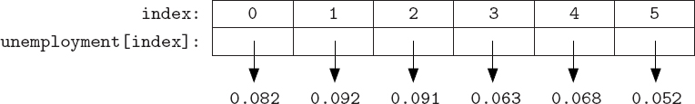
So the value 0.082 is assigned to the name unemployment[0], the value 0.092 is assigned to the name unemployment[1], etc. When we assigned a new value to unemployment[1] with unemployment[1] = 0.062, we were simply assigning a new value to the name unemployment[1], like any other assignment statement:
Suppose we wanted to adjust all of the unemployment rates in this list by subtracting one percent from each of them. We can do this with a for loop that iterates over the indices of the list.
>>> for index in range(len(unemployment)):
        unemployment[index] = unemployment[index] - 0.01
>>> unemployment
[0.072, 0.052, 0.081, 0.053, 0.058, 0.042]
This for loop is simply equivalent to the following six statements:
unemployment[0] = unemployment[0] - 0.01
unemployment[1] = unemployment[1] - 0.01
unemployment[2] = unemployment[2] - 0.01
unemployment[3] = unemployment[3] - 0.01
unemployment[4] = unemployment[4] - 0.01
unemployment[5] = unemployment[5] - 0.01
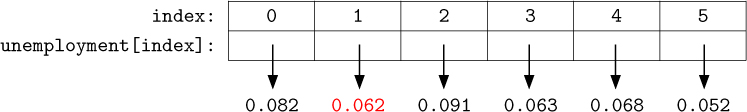
Reflection 8.7 Is it possible to achieve the same result by iterating over the values in the list instead? In other words, does the following for loop accomplish the same thing? (Try it.) Why or why not?
for rate in unemployment:
    rate = rate - 0.01
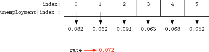
This loop does not modify the list because rate, which is being modified, is not a name in the list. So, although the value assigned to rate is being modified, the list itself is not. For example, at the beginning of the first iteration, 0.082 is assigned to rate, as illustrated below.

Then, when the modified value rate - 0.01 is assigned to rate, this only affects rate, not the original list, as illustrated below.
List parameters are mutable too
Now let’s put the correct loop above in a function named adjust that takes a list of unemployment rates as a parameter. We can then call the function with an actual list of unemployment rates that we wish to modify:
def adjust(rates):
    """Subtract one percent (0.01) from each rate in a list.

    Parameter:
        rates: a list of numbers representing rates (percentages)
    Return value: None
    """

    for index in range(len(rates)):
        rates[index] = rates[index] - 0.01

def main():
    unemployment = [0.053, 0.071, 0.065, 0.074]
    adjust(unemployment)
    print(unemployment)

main()
The list named unemployment is assigned in the main function and then passed in for the parameter rates to the adjust function. Inside the adjust function, every value in rates is decremented by 0.01. What effect, if any, does this have on the list assigned to unemployment? To find out, we need to look carefully at what happens when the function is called.
Right after the assignment statement in the main function, the situation looks like the following, with the variable named unemployment in the main namespace assigned the list [0.053, 0.071, 0.065, 0.074].
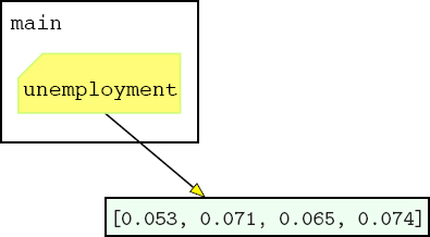
Now recall from Section 3.5 that, when an argument is passed to a function, it is assigned to its associated parameter. Therefore, immediately after the adjust function is called from main, the parameter rates is assigned the same list as unemployment:

After adjust executes, 0.01 has been subtracted from each value in rates, as the following picture illustrates.
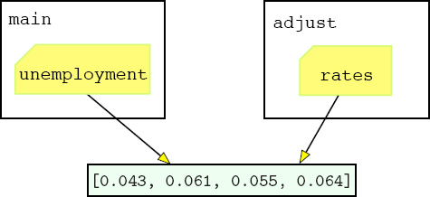
But notice that, since the same list is assigned to unemployment, these changes will also be reflected in the value of unemployment back in the main function. In other words, after the adjust function returns, the picture looks like this:

So when unemployment is printed at the end of main, the adjusted list [0.043, 0.061, 0.055, 0.064] will be displayed.
Reflection 8.8 Why does the argument’s value change in this case when it did not in the parameter passing examples in Section 3.5? What is different?
The difference here is that lists are mutable. When you pass a mutable value as an argument, any changes to the associated formal parameter inside the function will be reflected in the value of the argument. Therefore, when we pass a list as an argument to a function, the values in the list can be changed inside the function.
What if we did not want to change the argument to the adjust function (i.e., unemployment), and instead return a new adjusted list? One alternative, illustrated in the function below, would be to make a copy of rates, using the list method copy, and then modify this copy instead.
def adjust(rates):
    """ (docstring omitted) """

    ratesCopy = rates.copy()
    for index in range(len(ratesCopy)):
        ratesCopy[index] = ratesCopy[index] - 0.01
    return ratesCopy
The copy method creates an independent copy of the list in memory, and returns a reference to this new list so that it can be assigned to a variable name (in this case, ratesCopy). There are other solutions to this problem as well, which we leave as exercises.
Tuples
Python offers another list-like object called a tuple. A tuple works just like a list, with two substantive differences. First, a tuple is enclosed in parentheses instead of square brackets. Second, a tuple is immutable. For example, as a tuple, the unemployment data would look like (0.053, 0.071, 0.065, 0.074).
Tuples can be used in place of lists in situations where the object being represented has a fixed length, and individual components are not likely to change. For example, colors are often represented by their (red, green, blue) components (see Box 3.2) and two-dimensional points by (x, y).
>>> point = (4, 2)
>>> point
(4,   2)
>>> green = (0, 255, 0)
Reflection 8.9 Try reassigning the first value in point to 7. What happens?
>>> point[0] = 7
TypeError: 'tuple' object does not support item assignment
Tuples are more memory efficient than lists because extra memory is set aside in a list for a few appends before more memory must be allocated.
List operators and methods
Two operators that we used to create new strings can also be used to create new lists. The repetition operator * creates a new list that is built from repeats of the contents of a smaller list. For example:
>>> empty = [0] * 5
>>> empty
[0, 0, 0, 0, 0]
>>> ['up', 'down'] * 4
['up', 'down', 'up', 'down', 'up', 'down', 'up', 'down']
The concatenation operator + creates a new list that is the result of “sticking” two lists together. For example:
>>> unemployment = [0.082, 0.092, 0.091, 0.063, 0.068, 0.052]
>>> unemployment = unemployment + [0.087, 0.101]
>>> unemployment
[0.082, 0.092, 0.091, 0.063, 0.068, 0.052, 0.087, 0.101]
Notice that the concatenation operator combines two lists to create a new list, whereas the append method inserts a new element into an existing list as the last element. In other words,
unemployment = unemployment + [0.087, 0.101]
accomplishes the same thing as the two statements
unemployment.append(0.087)
unemployment.append(0.101)
However, using concatenation actually creates a new list that is then assigned to unemployment, whereas using append modifies an existing list. So using append is usually more efficient than concatenation if you are just adding to the end of an existing list.
Reflection 8.10 How do the results of the following two statements differ? If you want to add the number 0.087 to the end of the list, which is correct?
unemployment.append(0.087)
and
unemployment.append([0.087])
The list class has several useful methods in addition to append. We will use many of these in the upcoming sections to solve a variety of problems. For now, let’s look at four of the most common methods: sort, insert, pop, and remove.
The sort method simply sorts the elements in a list in increasing order. For example, suppose we have a list of SAT scores that we would like to sort:
>>> scores = [620, 710, 520, 550, 640, 730, 600]
>>> scores.sort()
>>> scores
[520, 550, 600, 620, 640, 710, 730]
Note that the sort and append methods, as well as insert, pop and remove, do not return new lists; instead they modify the lists in place. In other words, the following is a mistake:
>>> scores = [620, 710, 520, 550, 640, 730, 600]
>>> newScores = scores.sort()
Reflection 8.11 What is the value of newScores after we execute the statement above?
Printing the value of newScores reveals that it refers to the value None because sort does not return anything (meaningful). However, scores was modified as we expected:
>>> newScores
>>> scores
[520, 550, 600, 620, 640, 710, 730]
The sort method will sort any list that contains comparable items, including strings. For example, suppose we have a list of names that we want to be in alphabetical order:
>>> names = ['Eric', 'Michael', 'Connie', 'Graham']
>>> names.sort()
>>> names
['Connie', 'Eric', 'Graham', 'Michael']
Reflection 8.12 What happens if you try to sort a list containing items that cannot be compared to each other? For example, try sorting the list [3, 'one', 4, 'two'].
The insert method inserts an item into a list at a particular index. For example, suppose we want to insert new names into the sorted list above to maintain alphabetical order:
    >>> names.insert(3, 'John')
    >>> names
    ['Connie', 'Eric', 'Graham', 'John', 'Michael']
    >>> names.insert(0, 'Carol')
    >>> names
    ['Carol', 'Connie', 'Eric', 'Graham', 'John', 'Michael']
The first parameter of the insert method is the index where the inserted item will reside after the insertion.
The pop method is the inverse of insert; pop deletes the list item at a given index and returns the deleted value. For example,
      >>> inMemoriam = names.pop(3)
      >>> names
      ['Carol', 'Connie', 'Eric', 'John', 'Michael']
      >>> inMemoriam
      'Graham'
If the argument to pop is omitted, pop deletes and returns the last item in the list.
The remove method also deletes an item from a list, but takes the value of an item as its parameter rather than its position. If there are multiple items in the list with the given value, the remove method only deletes the first one. For example,
      >>> names.remove('John')
      >>> names
      ['Carol', 'Connie', 'Eric', 'Michael']
Reflection 8.13 What happens if you try to remove 'Graham' from names now?
*List comprehensions
As we mentioned at the beginning of this section, the list accumulator pattern is so common that there is a shorthand for it called a list comprehension. A list comprehension allows us to build up a list in a single statement. For example, suppose we wanted to create a list of the first 15 even numbers. Using a for loop, we can construct the desired list with:
      evens = [ ]
      for i in range(15):
          evens.append(2 * i)
An equivalent list comprehension looks like this:
evens = [2 * i for i in range(15)]
The first part of the list comprehension is an expression representing the items we want in the list. This is the same as the expression that would be passed to the append method if we constructed the list the “long way” with a for loop. This expression is followed by a for loop clause that specifies the values of an index variable for which the expression should be evaluated. The for loop clause is also identical to the for loop that we would use to construct the list the “long way.” This correspondence is illustrated below:
NumPy is a Python module that provides a different list-like class named array. (Because the numpy module is required by the matplotlib module, you should already have it installed.) Unlike a list, a NumPy array is treated as a mathematical vector. There are several different ways to create a new array. We will only illustrate two:
       >>> import numpy
       >>> a = numpy.array([1, 2, 3, 4, 5])
       >>> print(a)
       [1 2 3 4 5]
       >>> b = numpy.zeros(5)
       >>> print(b)
       [ 0. 0. 0. 0. 0.]
In the first case, a was assigned an array created from a list of numbers. In the second, b was assigned an array consisting of 5 zeros. One advantage of an array over a list is that arithmetic operations and functions are applied to each of an array object’s elements individually. For example:
       >>> print(a * 3)
       [ 3 6 9 12 15]
       >>> c = numpy.array([3, 4, 5, 6, 7])
       >>> print(a + c)
       [ 4 6 8 10 12]
There are also many functions and methods available to array objects. For example:
       >>> print(c.sum())
       25
       >>> print(numpy.sqrt(c))
       [ 1.73205081 2.           2.23606798   2.44948974   2.64575131]
An array object can also have more than one dimension, as we will discuss in Chapter 9. If you are interested in learning more about NumPy, visit http://www.numpy.org.

List comprehensions can also incorporate if statements. For example, suppose we wanted a list of the first 15 even numbers that are not divisible by 6. A for loop to create this list would look just like the previous example, with an additional if statement that checks that 2 * i is not divisible by 6 before appending it:
      evens = [ ]
      for i in range(15):
          if 2 * i % 6 != 0:
              evens.append(2 * i)
This can be reproduced with a list comprehension that looks like this:
evens = [2 * i for i in range(15) if 2 * i % 6 != 0]
The corresponding parts of this loop and list comprehension are illustrated below:

In general, the initial expression in a list comprehension can be followed by any sequence of for and if clauses that specify the values for which the expression should be evaluated.
Reflection 8.14 Rewrite the find function on Page 361 using a list comprehension.
The find function can be rewritten with the following list comprehension.
def find(text, target):
    """ (docstring omitted) """

    return [index for index in range(len(text) - len(target) + 1)
            if text[index:index + len(target)] == target]
Look carefully at the corresponding parts of the original loop version and the list comprehension version, as we did above.
Exercises
8.2.1. Show how to add the string 'grapes' to the end of the following list using both concatenation and the append method.
fruit = ['apples', 'pears', 'kiwi']
squares(n)
that returns a list containing the squares of the integers 1 through n. Use a for loop.
8.2.3. (This exercise assumes that you have read Section 6.7.) Write a function
getCodons(dna)
that returns a list containing the codons in the string dna. Your algorithm should use a for loop.
8.2.4. Write a function
square(data)
that takes a list of numbers named data and squares each number in data in place. The function should not return anything. For example, if the list [4, 2, 5] is assigned to a variable named numbers then, after calling square(numbers), numbers should have the value [16, 4, 25].
swap(data, i, j)
that swaps the positions of the items with indices i and j in the list named data.
8.2.6. Write a function
reverse(data)
that reverses the list data in place. Your function should not return anything. (Hint: use the swap function you wrote above.)
8.2.7. Suppose you are given a list of 'yea' and 'nay' votes. Write a function
winner(votes)
that returns the majority vote. For example, winner(['yea', 'nay', 'yea']) should return 'yea'. If there is a tie, return 'tie'.
8.2.8. Write a function
delete(data, index)
that returns a new list that contains the same elements as the list data except for the one at the given index. If the value of index is negative or exceeds the length of data, return a copy of the original list. Do not use the pop method. For example, delete([3, 1, 5, 9], 2) should return the list [3, 1, 9].
8.2.9. Write a function
remove(data, value)
that returns a new list that contains the same elements as the list data except for those that equal value. Do not use the builit-in remove method. Note that, unlike the built-in remove method, your function should remove all items equal to value. For example, remove([3, 1, 5, 3, 9], 3) should return the list [1, 5, 9].
8.2.10. Write a function
centeredMean(data)
that returns the average of the numbers in data with the largest and smallest numbers removed. You may assume that there are at least three numbers in the list. For example, centeredMean([2, 10, 3, 5]) should return 4.
8.2.11. On Page 365, we showed one way to write the adjust function so that it returned an adjusted list rather than modifying the original list. Give another way to accomplish the same thing.
8.2.12. Write a function
shuffle(data)
that shuffles the items in the list named data in place, without using the shuffle function from the random module. Instead, use the swap function you wrote in Exercise 8.2.5 to swap 100 pairs of randomly chosen items. For each swap, choose a random index for the first item and then choose a greater random index for the second item.
8.2.13. We wrote the following loop on Page 362 to subtract 0.01 from each value in a list:
             for index in range(len(unemployment)):
                 unemployment[index] = unemployment[index] - 0.01
Carefully explain why the following loop does not accomplish the same thing.
             for rate in unemployment:
                 rate = rate - 0.01
smooth(data, windowLength)
that returns a new list that contains the values in the list data, averaged over a window of the given length. This is the problem that we originally introduced in Section 1.3.
8.2.15. Write a function
median(data)
that returns the median number in a list of numbers named data.
8.2.16. Consider the following alphabetized grocery list:
groceries = ['cookies', 'gum', 'ham', 'ice cream', 'soap']
Show a sequence of calls to list methods that insert each of the following into their correct alphabetical positions, so that the final list is alphabetized:
'jelly beans''donuts''bananas''watermelon'
Next, show a sequence of calls to the pop method that delete each of the following items from the final list above.
'soap''watermelon''bananas''ham'
8.2.17. Given n people in a room, what is the probability that at least one pair of people shares a birthday? To answer this question, first write a function
sameBirthday(people)
that creates a list of people random birthdays and returns True if two birthdays are the same, and False otherwise. Use the numbers 0 to 364 to represent 365 different birthdays. Next, write a function
birthdayProblem(people, trials)
that performs a Monte Carlo simulation with the given number of trials to approximate the probability that, in a room with the given number of people, two people share a birthday.
8.2.18. Write a function that uses your solution to the previous problem to return the smallest number of people for which the probability of a pair sharing a birthday is at least 0.5.
8.2.19. Rewrite the squares function from Exercise 8.2.2 using a list comprehension.
8.2.20. (This exercise assumes that you have read Section 6.7.) Rewrite the getCodons function from Exercise 8.2.3 using a list comprehension.
8.3 FREQUENCIES, MODES, AND HISTOGRAMS
In addition to the mean and range of a list of data, which are single values, we might want to learn how data values are distributed throughout the list. The number of times that a value appears in a list is called its frequency. Once we know the frequencies of values in a list, we can represent them visually with a histogram and find the most frequent value(s), called the mode(s).
Tallying values
To get a sense of how we might compute the frequencies of values in a list, let’s consider the ocean buoy temperature readings that we first encountered in Chapter 1. As we did then, let’s simplify matters by just considering one week’s worth of data:
temperatures = [18.9, 19.1, 18.9, 19.0, 19.3, 19.2, 19.3]
Now we want to iterate over the list, keeping track of the frequency of each value that we see. We can imagine using a simple table for this purpose. After we see the first value in the list, 18.9, we create an entry in the table for 18.9 and mark its frequency with a tally mark.

The second value in the list is 19.1, so we create another entry and tally mark.

The third value is 18.9, so we add another tally mark to the 18.9 column.

The fourth value is 19.0, so we create another entry in the table with a tally mark.
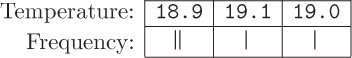
Continuing in this way with the rest of the list, we get the following final table.

Or, equivalently:

Now to find the mode, we find the maximum frequency in the table, and then return a list of the values with this maximum frequency: [18.9, 19.3].
Dictionaries
Notice how the frequency table resembles the picture of a list on Page 361, except that the indices are replaced by temperatures. In other words, the frequency table looks like a generalized list in which the indices are replaced by values that we choose. This kind of abstract data type is called a dictionary. In a dictionary, each index is replaced with a more general key. Unlike a list, in which the indices are implicit, a dictionary in Python (called a dict object) must define the correspondence between a key and its value explicitly with a key:value pair. To differentiate it from a list, a dictionary is enclosed in curly braces ({ }). For example, the frequency table above would be represented in Python like this:
>>> frequency = {18.9: 2, 19.1: 1, 19.0: 1, 19.2: 1, 19.3: 2}
The first pair in frequency has key 18.9 and value 2, the second item has key 19.1 and value 1, etc.
If you type the dictionary above in the Python shell, and then display it, you might notice something unexpected:
>>> frequency
{19.0: 1, 19.2: 1, 18.9: 2, 19.1: 1, 19.3: 2}
The items appear in a different order than they were originally. This is okay because a dictionary is an unordered collection of pairs. The displayed ordering has to do with the way dictionaries are implemented, using a structure called a hash table. If you are interested, you can learn a bit more about hash tables in Box 8.2.
Each entry in a dictionary object can be referenced using the familiar indexing notation, but using a key in the square brackets instead of an index. For example:
>>> frequency[19.3]
2
>>> frequency[19.1]
1
As we alluded to above, the model of a dictionary in memory is similar to a list (except that there is no significance attached to the ordering of the key values):

Each entry in the dictionary is a reference to a value in the same way that each entry in a list is a reference to a value. So, as with a list, we can change any value in a dictionary. For example, we can increment the value associated with the key 19.3:
>>> frequency[19.3] = frequency[19.3] + 1
Now let’s use a dictionary to implement the algorithm that we developed above to find frequencies and the mode(s) of a list. To begin, we will create an empty dictionary named frequency in which to record our tally marks:
def mode(data):
    """Compute the mode of a non-empty list.

    Parameter:
        data: a list of items

    Return value: the mode of the items in data
    """

    frequency = { }
A Python dictionary is implemented with a structure called a hash table. A hash table contains a fixed number of indexed slots in which the key:value pairs are stored. The slot assigned to a particular key:value pair is determined by a hash function that “translates” the key to a slot index. The picture below shows how some items in the frequency dictionary might be placed in an underlying hash table.
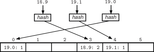
In this illustration, the hash function associates the pair 18.9: 2 with slot index 3, 19.1: 1 with slot index 4, and 19.0: 1 with slot index 0.
The underlying hash table allows us to access a value in a dictionary (e.g., frequency[18.9]) or test for inclusion (e.g., key in frequency) in a constant amount of time because each operation only involves a hash computation and then a direct access (like indexing in a string or a list). In contrast, if the pairs were stored in a list, then the list would need to be searched (in linear time) to perform these operations.
Unfortunately, this constant-time access could be foiled if a key is mapped to an occupied slot, an event called a collision. Collisions can be resolved by using adjacent slots, using a second hash function, or associating a list of items with each slot. A good hash function tries to prevent collisions by assigning slots in a seemingly random manner, so that keys are evenly distributed in the table and similar keys are not mapped to the same slot. Because hash functions tend to be so good, we can still consider an average dictionary access to be a constant-time operation, or one elementary step, even with collisions.
Each entry in this dictionary will have its key equal to a unique item in data and its value equal to the item’s frequency count. To tally the frequencies, we need to iterate over the items in data. As in our tallying algorithm, if there is already an entry in frequency with a key equal to the item, we will increment the item’s associated value; otherwise, we will create a new entry with frequency[item] = 1. To differentiate between the two cases, we can use the in operator: item in frequency evaluates to True if there is a key equal to item in the dictionary named frequency.
       for item in data:
           if item in frequency:    # item is already a key in frequency
               frequency[item] = frequency[item] + 1 # count the item
           else:
               frequency[item] = 1 # create a new entry item: 1
The next step is to find the maximum frequency in the dictionary. Since the frequencies are the values in the dictionary, we need to extract a list of the values, and then find the maximum in this list. A list of the values in a dictionary object is returned by the values method, and a list of the keys is returned by the keys method. For example, if we already had the complete frequency dictionary for the example above, we could extract the values with
>>> frequency.values()
dict_values([1, 1, 2, 1, 2])
The values method returns a special kind of object called a dict_values object, but we want the values in a list. To convert the dict_values object to a list, we simply use the list function:
>>> list(frequency.values())
[1, 1, 2, 1, 2]
We can get a list of keys from a dictionary in a similar way:
    >>> list(frequency.keys())
    [19.0, 19.2, 18.9, 19.1, 19.3]
The resulting lists will be in whatever order the dictionary happened to be stored, but the values and keys methods are guaranteed to produce lists in which every key in a key:value pair is in the same position in the list of keys as its corresponding value is in the list of values.
Returning to the problem at hand, we can use the values method to retrieve the list of frequencies, and then find the maximum frequency in that list:
      frequencyValues = list(frequency.values())
      maxFrequency = max(frequencyValues)
Finally, to find the mode(s), we need to build a list of all the items in data with frequency equal to maxFrequency. To do this, we iterate over all the keys in frequency, appending to the list of modes each key that has a value equal to maxFrequency. Iterating over the keys in frequency is done with the familiar for loop. When the for loop is done, we return the list of modes.
         modes = [ ]
         for key in frequency:
             if frequency[key] == maxFrequency:
                 modes.append(key)

         return modes
With all of these pieces in place, the complete function looks like the following.

Figure 8.1 A histogram displaying the frequency of each temperature reading in the list [18.9, 19.1, 18.9, 19.0, 19.3, 19.2, 19.3].
def mode(data):
    """ (docstring omitted) """

    frequency = { }

    for item in data:
        if item in frequency:
            frequency[item] = frequency[item] + 1
        else:
            frequency[item] = 1

    frequencyValues = list(frequency.values())
    maxFrequency = max(frequencyValues)

    modes = [ ]
    for key in frequency:
        if frequency[key] == maxFrequency:
            modes.append(key)

    return modes
As a byproduct of computing the mode, we have also done all of the work necessary to create a histogram for the values in data. The histogram is simply a vertical bar chart with the keys on the x-axis and the height of the bars equal to the frequency of each key. We leave the creation of a histogram as Exercise 8.3.7. As an example, Figure 8.1 shows a histogram for our temperatures list.
We can use dictionaries for a variety of purposes beyond counting frequencies. For example, as the name suggests, dictionaries are well suited for handling translations. The following dictionary associates a meaning with each of three texting abbreviations.
>>> translations = {'lol': 'laugh out loud', 'u': 'you', 'r': 'are'}
We can find the meaning of lol with
    >>> translations['lol']
    'laugh out loud'
There are more examples in the exercises that follow.
Exercises
printFrequencies(frequency)
that prints a formatted table of frequencies stored in the dictionary named frequency. The key values in the table must be listed in sorted order. For example, for the dictionary in the text, the table should look something like this:
             Key       Frequency
             18.9         2
             19.0         1
             19.1         1
             19.2         1
             19.3         2
(Hint: iterate over a sorted list of keys.)
8.3.2. Write a function
wordFrequency(text)
that returns a dictionary containing the frequency of each word in the string text. For example, wordFrequency('I am I.') should return the dictionary {'I': 2, 'am': 1}. (Hint: the split and strip string methods will be useful; see Appendix B.)
8.3.3. The probability mass function (PMF) of a data set gives the probability of each value in the set. A dictionary representing the PMF is a frequency dictionary with each frequency value divided by the total number of values in the original data set. For example, the probabilities for the values represented in the table in Exercise 8.3.1 are shown below.
             Key        Probability
             18.9          2/7
             19.0          1/7
             19.1          1/7
             19.2          1/7
             19.3          2/7
Write a function
pmf(frequency)
that returns a dictionary containing the PMF of the frequency dictionary passed as a parameter.
wordFrequencies(fileName)
that prints an alphabetized table of word frequencies in the text file with the given fileName.
firstLetterCount(words)
that takes as a parameter a list of strings named words and returns a dictionary with lower case letters as keys and the number of words in words that begin with that letter (lower or upper case) as values. For example, if the list is ['ant', 'bee', 'armadillo', 'dog', 'cat'], then your function should return the dictionary {'a': 2, 'b': 1, 'c': 1, 'd': 1}.
8.3.6. Similar to the Exercise 8.3.5, write a function
firstLetterWords(words)
that takes as a parameter a list of strings named words and returns a dictionary with lower case letters as keys. But now associate with each key the list of the words in words that begin with that letter. For example, if the list is ['ant', 'bee', 'armadillo', 'dog', 'cat'], then your function should return the dictionary {'a': ['ant', 'armadillo'], 'b': ['bee'], 'c': ['cat'], 'd': ['dog']}.
histogram(data)
that displays a histogram of the values in the list data using the bar function from matplotlib. The matplotlib function bar(x, heights, align = 'center') draws a vertical bar plot with bars of the given heights, centered at the x-coordinates in x. The bar function defines the widths of the bars with respect to the range of values on the x-axis. Therefore, if frequency is the name of your dictionary, it is best to pass in range(len(frequency)), instead of list(frequency.keys()), for x. Then label the bars on the x-axis with the matplotlib function xticks(range(len(frequency)), list(frequency.keys())).
8.3.8. Write a function
bonus(salaries)
that takes as a parameter a dictionary named salaries, with names as keys and salaries as values, and increases the salary of everyone in the dictionary by 5%.
8.3.9. Write a function
updateAges(names, ages)
that takes as parameters a list of names of people whose birthday it is today and a dictionary named ages, with names as keys and ages as values, and increments the age of each person in the dictionary whose birthday is today.
8.3.10. Write a function
seniorList(students, year)
that takes as a parameter a dictionary named students, with names as keys and class years as values, and returns a list of names of students who are graduating in year.
8.3.11. Write a function
createDictionary()
that creates a dictionary, inserts several English words as keys and the Pig Latin (or any other language) translations as values, and then returns the completed dictionary.
Next write a function
translate()
that calls your createDictionary function to create a dictionary, and then repeatedly asks for a word to translate. For each entered word, it should print the translation using the dictionary. If a word does not exist in the dictionary, the function should say so. The function should end when the word quit is typed.
8.3.12. Write a function
txtTranslate(word)
that uses a dictionary to return the English meaning of the texting abbreviation word. Incorporate translations for at least ten texting abbreviations. If the abbreviation is not in the dictionary, your function should return a suitable string message instead. For example, txtTranslate('lol') might return 'laugh out loud'.
login(passwords)
that takes as a parameter a dictionary named passwords, with usernames as keys and passwords as values, and repeatedly prompts for a username and password until a valid pair is entered. Your function should continue to prompt even if an invalid username is entered.
8.3.14. Write a function
union(dict1, dict2)
that returns a new dictionary that contains all of the entries of the two dictionaries dict1 and dict2. If the dictionaries share a key, use the value in the first dictionary. For example, union({'pies': 3, 'cakes': 5}, {'cakes': 4, 'tarts': 2} should return the dictionary {'pies': 3, 'cakes': 5, 'tarts': 2}.
8.3.15. The Mohs hardness scale rates the hardness of a rock or mineral on a 10-point scale, where 1 is very soft (like talc) and 10 is very hard (like diamond). Suppose we have a list such as
rocks = [('talc', 1), ('lead', 1.5), ('copper', 3),
         ('nickel', 4), ('silicon', 6.5), ('emerald', 7.5),
         ('boron', 9.5), ('diamond', 10)]
where the first element of each tuple is the name of a rock or mineral, and the second element is its hardness. Write a function
hardness(rocks)
that returns a dictionary organizing the rocks and minerals in such a list into four categories: soft (1–3), medium (3.1–5), hard (5.1–8), and very hard (8.1–10). For example, given the list above, the function would return the dictionary
{'soft': ['talc', 'lead', 'copper'],
 'medium': ['nickel'],
 'hard': ['silicon', 'emerald'],
 'very hard': ['boron', 'diamond']}
8.3.16. (This exercise assumes that you have read Section 6.7.) Rewrite the complement function on page 302 using a dictionary. (Do not use any if statements.)
8.3.17. (This exercise assumes that you have read Section 6.7.) Suppose we have a set of homologous DNA sequences with the same length. A profile for these sequences contains the frequency of each base in each position. For example, suppose we have the following five sequences, lined up in a table:
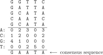
Their profile is shown below the sequences. The first column of the profile indicates that there is one sequence with a C in its first position and four sequences with a G in their first position. The second column of the profile shows that there are two sequences with A in their second position, two sequences with C in their second position, and one sequence with G in its second position. And so on. The consensus sequence for a set of sequences has in each position the most common base in the profile. The consensus for this list of sequences is shown below the profile.
A profile can be implemented as a list of 4-element dictionaries, one for each column. A consensus sequence can then be constructed by finding the base with the maximum frequency in each position. In this exercise, you will build up a function to find a consensus sequence in four parts.
- Write a function
profile1(sequences, index)
that returns a dictionary containing the frequency of each base in position
indexin the list of DNA sequences namedsequences. For example, suppose we pass in the list['GGTTC', 'GATTA', 'GCATA', 'CAATC', 'GCATA']forsequences(the sequences from the example above) and the value 2 forindex. Then the function should return the dictionary{'A': 3, 'C': 0, 'G': 0, 'T': 2}, equivalent to the third column in the profile above. - Write a function
profile(sequences)
that returns a list of dictionaries representing the profile for the list of DNA sequences named
sequences. For example, given the list of sequences above, the function should return the list[{'A': 0, 'C': 1, 'G': 4, 'T': 0},
{'A': 2, 'C': 2, 'G': 1, 'T': 0},
{'A': 3, 'C': 0, 'G': 0, 'T': 2},
{'A': 0, 'C': 0, 'G': 0, 'T': 5},
{'A': 3, 'C': 2, 'G': 0, 'T': 0}]Your
profilefunction should call yourprofile1function in a loop. - Write a function
maxBase(freqs)
that returns the base with the maximum frequency in a dictionary of base frequencies named
freqs. For example,maxBase({'A': 0, 'C': 1, 'G': 4, 'T': 0})should return
'G'. - Write a function
consensus(sequences)
that returns the consensus sequence for the list of DNA sequences named
sequences. Yourconsensusfunction should call yourprofilefunction and also call yourmaxBasefunction in a loop.
8.4 READING TABULAR DATA
In Section 6.2, we read one-dimensional text from files and designed algorithms to analyze the text in various ways. A lot of data, however, is maintained in the form of two-dimensional tables instead. For example, the U.S. Geological Survey (USGS) maintains up-to-the-minute tabular data about earthquakes happening around the world at http://earthquake.usgs.gov/earthquakes/feed/v1.0/csv.php. Earthquakes typically occur on the boundaries between tectonic plates. Therefore, by extracting this data into a usable form, and then plotting the locations of the earthquakes with matplotlib, we can visualize the locations of the earth’s tectonic plates.
The USGS earthquake data is available in many formats, the simplest of which is called CSV, short for “comma-separated values.” The first few columns of a USGS data file look like the following.
time,latitude,longitude,depth,mag,magType,...
2013-09-24T20:01:22.700Z,40.1333,-123.863,29,1.8,Md,...
2013-09-24T18:57:59.000Z,59.8905,-151.2392,56.4,2.5,Ml,...
2013-09-24T18:51:19.100Z,37.3242,-122.1015,0.3,1.8,Md,...
2013-09-24T18:40:09.100Z,34.3278,-116.4663,8.5,1.2,Ml,...
2013-09-24T18:20:06.300Z,35.0418,-118.3227,1.3,1.4,Ml,...
2013-09-24T18:09:53.700Z,32.0487,-115.0075,28,3.2,Ml,...
As you can see, CSV files contain one row of text per line, with columns separated by commas. The first row contains the names of the fifteen columns in this file, only six of which are shown here. Each additional row consists of fifteen columns of data from one earthquake. The first earthquake in this file was first detected at 20:01 UTC (Coordinated Universal Time) on 2013-09-24 at 40.1333 degrees latitude and –123.863 degrees longitude. The earthquake occurred at a depth of 29 km and had magnitude 1.8.
The CSV file containing data about all of the earthquakes in the past month is available on the web at the URL
http://earthquake.usgs.gov/earthquakes/feed/v1.0/summary/all_month.csv
(If you have trouble with this file, you can try smaller files by replacing all_month with 2.5_month or 4.5_month. The numbers indicate the minimum magnitude of the earthquakes included in the file.)
Reflection 8.15 Enter the URL above into a web browser to see the data file for yourself. About how many earthquakes were recorded in the last month?
We can read the contents of CSV files in Python using the same techniques that we used in Section 6.2. We can either download and save this file manually (and then read the file from our program), or we can download it directly from our program using the urllib.request module. We will use the latter method.
To begin our function, we will open the URL, and then read the header row containing the column names, as follows. (We do not actually need the header row; we just need to get past it to get to the data.)
import urllib.request as web

def plotQuakes():
    """Plot the locations of all earthquakes in the past month.

    Parameters: None

    Return value: None
    """


    url = 'http://earthquake.usgs.gov/...' # see above for full URL
    quakeFile = web.urlopen(url)
    header = quakeFile.readline()
To visualize fault boundaries with matplotlib, we will need all the longitude (x) values in one list and all the latitude (y) values in another list. In our plot, we will color the points according to their depths, so we will also need to extract the depths of the earthquakes in a third list. To maintain an association between the latitude, longitude, and depth of a particular earthquake, we will need these lists to be parallel in the sense that, at any particular index, the longitude, latitude, and depth at that index belong to the same earthquake. In other words, if we name these three lists longitudes, latitudes, and depths, then for any value of index, longitudes[index], latitudes[index], and depths[index] belong to the same earthquake.
In our function, we next initialize these three lists to be empty and begin to iterate over the lines in the file:
longitudes = []
latitudes = []
depths = []
for line in quakeFile:
    line = line.decode('utf-8')
To extract the necessary information from each line of the file, we can use the split method from the string class. The split method splits a string at every instance of a given character, and returns a list of strings that result. For example, 'this;is;a;line'.split(';') returns the list of strings ['this', 'is', 'a', 'line']. (If no argument is given, it splits at strings of whitespace characters.) In this case, we want to split the string line at every comma:
row = line.split(',')
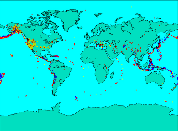
Figure 8.2 Plotted earthquake locations with colors representing depths (yellow dots are shallower, red dots are medium, and blue dots are deeper).
The resulting list named row will have the time of the earthquake at index 0, the latitude at index 1, the longitude at index 2 and the depth at index 3, followed by 11 additional columns that we will not use. Note that each of these values is a string, so we will need to convert each one to a number using the float function. After converting each value, we append it to its respective list:
         latitudes.append(float(row[1]))
         longitudes.append(float(row[2]))
         depths.append(float(row[3]))
Finally, after the loop completes, we close the file.
quakeFile.close()
Once we have the data from the file in this format, we can plot the earthquake epicenters, and depict the depth of each earthquake with a color. Shallow (less than 10 km deep) earthquakes will be yellow, medium depth (between 10 and 50 km) earthquakes will be red, and deep earthquakes (greater than 50 km deep) will be blue. In matplotlib, we can color each point differently by passing the scatter function a list of colors, one for each point. To create this list, we iterate over the depths list and, for each depth, append the appropriate color string to another list named colors:
    colors = []
    for depth in depths:
        if depth < 10:
             colors.append('yellow')
        elif depth < 50:
             colors.append('red')
        else:
             colors.append('blue')
Finally, we can plot the earthquakes in their respective colors:
    pyplot.scatter(longitudes, latitudes, 10, color = colors)
    pyplot.show()
In the call to scatter above, the third argument is the square of the size of the point marker, and color = colors is a keyword argument. (We also saw keyword arguments briefly in Section 4.1.) The name color is the name of a parameter of the scatter function, for which we are passing the argument colors. (We will only use keyword arguments with matplotlib functions, although we could also use them in our functions if we wished to do so.)
The complete plotQuakes function is shown below.
import urllib.request as web
import matplotlib.pyplot as pyplot

def plotQuakes():
    """Plot the locations of all earthquakes in the past month.

    Parameters: None

    Return value: None
    """

    url = 'http://earthquake.usgs.gov/...' # see above for full URL
    quakeFile = web.urlopen(url)
    header = quakeFile.readline()

    longitudes = []
    latitudes = []
       depths = []
    for line in quakeFile:
        line = line.decode('utf-8')
        row = line.split(',')
        latitudes.append(float(row[1]))
        longitudes.append(float(row[2]))
        depths.append(float(row[3]))
   quakeFile.close()

   colors = []
   for depth in depths:
       if depth < 10:
           colors.append('yellow')
       elif depth < 50:
           colors.append('red')
       else:
           colors.append('blue')

   pyplot.scatter(longitudes, latitudes, 10, color = colors)
   pyplot.show()
The plotted earthquakes are shown in Figure 8.2 over a map background. (Your plot will not show the map, but if you would like to add it, look into the Basemap class from the mpl_toolkits.basemap module.) Geologists use illustrations like Figure 8.2 to infer the boundaries between tectonic plates.
Reflection 8.16 Look at Figure 8.2 and try to identify the different tectonic plates. Can you infer anything about the way neighboring plates interact from the depth colors?
For example, the ring of red and yellow dots around Africa encloses the African plate, and the dense line of blue and red dots northwest of Australia delineates the boundary between the Eurasian and Australian plates. The depth information gives geologists information about the types of the boundaries and the directions in which the plates are moving. For example, the shallow earthquakes on the west coast of North America mark a divergent boundary in which the plates are moving away from each other, while the deeper earthquakes in the Aleutian islands near Alaska mark a subduction zone on a convergent boundary where the Pacific plate to the south is diving underneath the North American plate to the north.
Exercises
8.4.1. Modify plotQuakes so that it also reads earthquake magnitudes into a list, and then draws larger circles for higher magnitude earthquakes. The sizes of the circles can be changed by passing a list of sizes, similar to the list of colors, as the third argument to the scatter function.
8.4.2. Modify the function from Exercise 8.3.5 so that it takes a file name as a parameter and uses the words from this file instead. Test your function using the SCRABBLE® dictionary on the book web site.1
8.4.3. Modify the function from Exercise 8.3.13 so that it takes a file name as a parameter and creates a username/password dictionary with the usernames and passwords in that file before it starts prompting for a username and password. Assume that the file contains one username and password per line, separated by a space. There is an example file on the book web site.
8.4.4. Write a function
plotPopulation()
that plots the world population over time from the tab-separated data file on the book web site named worldpopulation.txt. To read a tab-separated file, split each line with line.split(' '). These figures are U.S. Census Bureau midyear population estimates from 1950–2050. Your function should create two plots. The first shows the years on the x-axis and the populations on the y-axis. The second shows the years on the x-axis and the annual growth rate on the y-axis. The growth rate is the difference between this year’s population and last year’s population, divided by last year’s population. Be sure to label your axes in both plots with the xlabel and ylabel functions. What is the overall trend in world population growth? Do you have any hypotheses regarding the most significant spikes and dips?
8.4.5. Write a function
plotMeteorites()
that plots the location (longitude and latitude) of every known meteorite that has fallen to earth, using a tab-separated data file from the book web site named meteoritessize.txt. Split each line of a tab-separated file with line.split(' '). There are large areas where no meteorites have apparently fallen. Is this accurate? Why do you think no meteorites show up in these areas?
plotTemps()
that reads a CSV data file from the book web site named madison_temp.csv to plot several years of monthly minimum temperature readings from Madison, Wisconsin. The temperature readings in the file are integers in tenths of a degree Celsius and each date is expressed in YYYYMMDD format. Rather than putting every date in a list for the x-axis, just make a list of the years that are represented in the file. Then plot the data and put a year label at each January tick with
pyplot.plot(range(len(minTemps)), minTemps)
pyplot.xticks(range(0, len(minTemps), 12), years)
The first argument to the xticks function says to only put a tick at every twelfth x value, and the second argument supplies the list of years to use to label those ticks. It will be helpful to know that the data file starts with a January 1 reading.
8.4.7. Write a function
plotZebras()
that plots the migration of seven Burchell’s zebra in northern Botswana. (The very interesting story behind this data can be found at https://www.movebank.org/node/11921.) The function should read a CSV data file from the book web site named zebra.csv. Each line in the data file is a record of the location of an individual zebra at a particular time. Each individual has a unique identifier. There are over 50,000 records in the file. For each record, your function should extract the individual identifier (column index 9), longitude (column index 3), and latitude (column index 4). Store the data in two dictionaries, each with a key equal to an identifier. The values in the two dictionaries should be the longitudes and latitudes, respectively, of all tracking events for the zebra with that identifier. Plot the locations of the seven zebras in seven different colors to visualize their migration patterns.
How can you determine from the data which direction the zebras are migrating?
8.4.8. On the book web site, there is a tab-separated data file named education.txt that contains information about the maximum educational attainment of U.S. citizens, as of 2013. Each non-header row contains the number of people in a particular category (in thousands) that have attained each of fifteen different educational levels. Look at the file in a text editor (not a spreadsheet program) to view its contents. Write a function
plotEducation()
that reads this data and then plots separately (but in one figure) the educational attainment of all males, females, and both sexes together over 18 years of age. The x-axis should be the fifteen different educational attainment levels and the y axis should be the percentage of each group that has attained that level. Notice that you will only need to extract three lines of the data file, skipping over the rest. To label the ticks on the x-axis, use the following:
pyplot.xticks(range(15), titles[2:], rotation = 270)
pyplot.subplots_adjust(bottom = 0.45)
The first statement labels the x ticks with the educational attainment categories, rotated 270 degrees. The second statement reserves 45% of the vertical space for these x tick labels. Can you draw any conclusions from the plot about relative numbers of men and women who pursue various educational degrees?
*8.5 DESIGNING EFFICIENT ALGORITHMS
For nearly all of the problems we have encountered so far, there has been only one algorithm, and its design has been relatively straightforward. But for most real problems that involve real data, there are many possible algorithms, and a little more ingenuity is required to find the best one.
To illustrate, let’s consider a slightly more involved problem that can be formulated in terms of the following “real world” situation. Suppose you organized a petition drive in your community, and have now collected all of the lists of signatures from your volunteers. Before you can submit your petition to the governor, you need to remove duplicate signatures from the combined list. Rather than try to do this by hand, you decide to scan all of the names into a file, and design an algorithm to remove the duplicates for you. Because the signatures are numbered, you want the final list of unique names to be in their original order.
As we design an algorithm for this problem, we will keep in mind the four steps outlined in Section 7.1:
Understand the problem.
Design an algorithm.
Implement your algorithm as a program.
Analyze your algorithm for clarity, correctness, and efficiency.
Reflection 8.17 Before you read any further, make sure you understand this problem. If you were given this list of names on paper, what algorithm would you use to remove the duplicates?
The input to our problem is a list of items, and the output is a new list of unique items in the same order they appeared in the original list. We will start with an intuitive algorithm and work through a process of refinement to get progressively better solutions. In this process, we will see how a critical look at the algorithms we write can lead to significant improvements.
A first algorithm
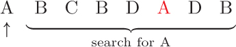
There are several different approaches we could use to solve this problem. We will start with an algorithm that iterates over the items and, for each one, marks any duplicates found further down the list. Once all of the duplicates are marked, we can remove them from a copy of the original list. The following example illustrates this approach with a list containing four unique names, abbreviated A, B, C, and D. The algorithm starts at the beginning of the list, which contains the name A. Then we search down the list and record the index of the duplicate, marked in red.
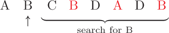
Next we move on to the second item, B, and mark its duplicates.
Some items, like the next item, C, do not have any duplicates.
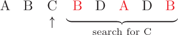
The item after C is already marked as a duplicate, so we skip the search.

The next item, D, is not marked so we search for its duplicates down the list.

Finally, we finish iterating over the list, but find that the remaining items are already marked as duplicates.
Once we know where all the duplicates are, we can make a copy of the original list and remove the duplicates from the copy. This algorithm, partially written in Python, is shown below. We keep track of the “marked” items with a list of their indices. The portions in red need to be replaced with calls to appropriate functions, which we will develop soon.
 1   def removeDuplicates1(data):
 2       """Return a list containing only the unique items in data.
 3
 4       Parameter:
 5           data: a list
 6
 7       Return value: a new list of the unique values in data,
 8                     in their original order
 9       """
10
11       duplicateIndices = [ ]        # indices of duplicate items
12       for index in range(len(data)):
13           if index is not in duplicateIndices:
14               positions = indices of later duplicates of data[index]
15               duplicateIndices.extend(positions)
16
17       unique = data.copy()
18       for index in duplicateIndices:
19           remove data[index] from unique
20
21       return unique
To implement the red portion of the if statement on line 13, we need to search for index in the list duplicateIndices. We could use the Python in operator (if index in duplicateIndices:), but let’s instead revisit how to write a search function from scratch. Recall that, in Section 6.5, we developed a linear search algorithm (named find) that returns the index of the first occurrence of a substring in a string. We can use this algorithm as a starting point for an algorithm to find an item in a list.
Reflection 8.18 Look back at the find function on Page 283. Modify the function so that it returns the index of the first occurrence of a target item in a list.
The linear search function, based on the find function but applied to a list, follows.
def linearSearch(data, target):
    """Find the index of the first occurrence of target in data.

    Parameters:
           data: a list object to search in
           target: an object to search for

    Return value: the index of the first occurrence of target in data
    """

    for index in range(len(data)):
          if data[index] == target:
               return index
    return -1
The function iterates over the indices of the list named data, checking whether each item equals the target value. If a match is found, the function returns the index of the match. Otherwise, if no match is ever found, the function returns –1. We can call this function in the if statement on line 13 of removeDuplicates1 to determine whether the current value of index is already in duplicateIndices.
Reflection 8.19 What would this if statement look like?
We want the condition in the if statement to be true if index is not in the list, i.e., if linearSearch returns –1. So the if statement should look like:
if linearSearch(duplicateIndices, index) == -1:
In the red portion on line 14, we need to find all of the indices of items equal to data[index] that occur later in the list. A function to do this will be very similar to linearSearch, but differ in two ways. First, it must return a list of indices instead of a single index. Second, it will require a third parameter that specifies where the search should begin.
Reflection 8.20 Write a new version of linearSearch that differs in the two ways outlined above.
The resulting function could look like this:
def linearSearchAll(data, target, start):
    """Find the indices of all occurrences of target in data.

    Parameters:
           data: a list object to search in
           target: an object to search for
           start: the index in data to start searching from

    Return value: a list of indices of all occurrences of
                  target in data
    """

    found = [ ]
    for index in range(start, len(data)):
        if data[index] == target:
            found.append(index)
    return found
With these two new functions, we can fill in the first two missing parts of our removeDuplicates1 function:
def removeDuplicates1(data):
    """ (docstring omitted) """

    duplicateIndices = [ ]        # indices of duplicate items
    for index in range(len(data)):
        if linearSearch(duplicateIndices, index) == -1:
            positions = linearSearchAll(data, data[index], index + 1)
            duplicateIndices.extend(positions)

    unique = data.copy()
    for index in duplicateIndices:
        remove data[index] from unique

    return unique
Once we have the list of duplicates, we need to remove them from the list. The algorithm above suggests using the pop method to do this, since pop takes an index as a parameter:
unique.pop(index)
However, this is likely to cause a problem. To see why, suppose we have the list [1, 2, 3, 2, 3] and we want to remove the duplicates at indices 3 and 4:
>>> data = [1, 2, 3, 2, 3]
>>> data.pop(3)
>>> data.pop(4)
Reflection 8.21 What is the problem above?
The problem is that, after we delete the item at index 3, the list looks like [1, 2, 3, 3], so the next item we want to delete is at index 3 instead of index 4. In fact, there is no index 4!
An alternative approach would be to use a list accumulator to build the unique list up from an empty list. To do this, we will need to iterate over the original list and append items to unique if their indices are not in duplicateIndices. The following function replaces the last loop with a new list accumulator loop that uses this approach instead.
def removeDuplicates1(data):
    """ (docstring omitted) """

    duplicateIndices = [ ]         # indices of duplicate items
    for index in range(len(data)):
        if linearSearch(duplicateIndices, index) == -1:
            positions = linearSearchAll(data, data[index], index + 1)
            duplicateIndices.extend(positions)

    unique = [ ]
    for index in range(len(data)):
        if linearSearch(duplicateIndices, index) == -1:
            unique.append(data[index])

   return unique
We now finally have a working function! (Try it out.) However, this does not mean that we should immediately leave this problem behind. It is important that we take some time to critically reflect on our solution. Is it correct? (If you covered Section 7.3, this would be a good time to develop some unit tests.) Can the function be simplified or made more efficient? What is the algorithm’s time complexity?
Reflection 8.22 The function above can be simplified a bit. Look at the similarity between the two for loops. Can they be combined?
The two for loops can, in fact, be combined. If the condition in the first if statement is true, then this must be the first time we have seen this particular list item. Therefore, we can append it to the unique list right then. The resulting function is a bit more streamlined:
 1   def removeDuplicates1(data):
 2       """ (docstring omitted) """
 3
 4       duplicateIndices = [ ]
 5       unique = [ ]
 6       for index in range(len(data)):
 7           if linearSearch(duplicateIndices, index) == -1:
 8               positions = linearSearchAll(data, data[index], index + 1)
 9               duplicateIndices.extend(positions)
10               unique.append(data[index])
11       return unique
Now let’s analyze the asymptotic time complexity of this algorithm in the worst case. The input to the algorithm is the parameter data. As usual, we will call the length of this list n (i.e., len(data) is n). The statements on lines 4, 5, and 11 each count as one elementary step. The rest of the algorithm is contained in the for loop, which iterates n times. So the if statement on line 7 is executed n times and, in the worst case, the statements on lines 8–10 are each executed n times as well. But how many elementary steps are hidden in each of these statements?
Reflection 8.23 How many elementary steps are required in the worst case by the call to linearSearch on line 7? (You might want to refer back to Page 283, where we talked about the time complexity of a linear search.)
We saw in Section 6.5 that linear search is a linear-time algorithm (hence the name). So the number of elementary steps required by line 7 is proportional to the length of the list that is passed in as a parameter. The length of the list that we pass into linearSearch in this case, duplicateIndices, will be zero in the first iteration of the loop, but may contain as many as n – 1 indices in the second iteration. So the total number of elementary steps in each of these later iterations is at most n – 1, which is just n asymptotically.
Reflection 8.24 Why could duplicateIndices have length n – 1 after the first iteration of the loop? What value of data would make this happen?
So the total number of elementary steps executed by line 7 is at most 1 + (n – 1)(n), one in the first iteration of the loop, then at most n for each iteration thereafter. This simplifies to n2 – n + 1 which, asymptotically, is just n2.
The linearSearchAll function, called on line 8, is also a linear search, but this function only iterates from start to the end of the list, so it requires about n – start elementary steps instead of n, as long as the call to append that is in the body of the loop qualifies as an elementary step.
Reflection 8.25 Do you think append qualifies as an elementary step? In other words, does it take the same amount of time regardless of the list or the item being appended?
Consider a typical call to the append method, like data.append(item). How many elementary steps are involved in this call? We have seen that some Python operations, like assignment statements, require a constant number of elementary steps while others, like the count method, can require a linear number of elementary steps. The append method is an interesting case because the number of elementary steps depends on how much space is available in the chunk of memory that has been allocated to hold the list. If there is room available at the end of this chunk of memory, then a reference to the appended item can be placed at the end of the list in constant time. However, if the list is already occupying all of the memory that has been allocated to it, the append has to allocate a larger chunk of memory, and then copy the entire list to this larger chunk. The amount of time to do this is proportional to the current length of the list. To reconcile these different cases, we can use the average number of elementary steps over a long sequence of append calls, a technique known as amortization.
When a new chunk of memory needs to be allocated, Python allocates more than it actually needs so that the next few append calls will be quicker. The amount of extra memory allocated is cleverly proportional to the length of the list, so the extra memory grows a little more each time. Therefore, a sequence of append calls on the same list will consist of sequences of several quick operations interspersed with increasingly rare slow operations. If you take the average number of elementary steps over all of these appends, it turns out to be a constant number (or very close to it). Thus an append can be considered one elementary step!
This is actually a tricky question to answer, as explained in Box 8.3. In a nutshell, the average time required over a sequence of append calls is constant (or close enough to it), so it is safe to characterize an append as an elementary step. So it is safe to say that a call to linearSearchAll requires about n – start elementary steps. When the linearSearchAll function is called on line 8, the value of index + 1 is passed in for start. So when index has the value 0, the linearSearchAll function requires about n – start = n – (index + 1) = n – 1 elementary steps. When index has the value 1, it requires about n – (index + 1) = n – 2 elementary steps. And so on. So the total number of elementary steps in line 8 is
(n – 1) + (n – 2) + ··· + 1.
We have seen this sum before (see Box 4.2); it is equal to the triangular number
which is the same as n2 asymptotically.
Finally, lines 9 and 10 involve a total of n elementary steps asymptotically. This is easier to see with line 10 because it involves at most one append per iteration. The extend method called on line 9 effectively appends all of the values in positions
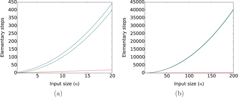
Figure 8.3 Two views of the time complexities n2 + 2n + 2 (blue), n2 (green), and n (red). (This is the same as Figure 6.4.)
to the end of duplicateIndices. Although one call to extend may append more than one index to duplicateIndices at a time, overall, each index of data can be appended at most once, so the total number of elementary steps over all of the calls to extend must be proportional to n. In summary, we have determined the following numbers of elementary steps for each line.
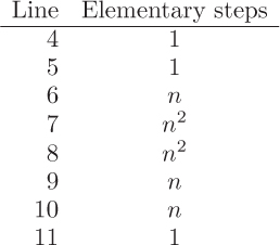
Since the maximum number of elementary steps for any line is n2, this is the asymptotic time complexity of the algorithm. Algorithms with asymptotic time complexity n2 are called quadratic-time algorithms.
How do quadratic-time algorithms compare to the linear-time algorithms we have encountered in previous chapters? The answer is communicated graphically by Figure 8.3: quadratic-time algorithms are a lot slower than linear-time algorithms. However, they still tend to finish in a reasonable amount of time, unless n is extremely large.
Another visual way to understand the difference between a linear-time algorithm and a quadratic-time algorithm is shown in Figure 8.4. Suppose each square represents one elementary step. On the left is a representation of the work required in a linear-time algorithm. If the size of the input to the linear-time algorithm
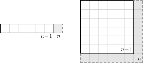
increases from n–1 to n (n = 7 in the pictures), then the algorithm must execute one additional elementary step (in gray). On the right is a representation of the work involved in a quadratic-time algorithm. If the size of the input to the quadratic-time algorithm increases from n– 1 to n, then the algorithm gains 2n – 1 additional steps. So we can see that the amount of work that a quadratic-time algorithm must do grows much more quickly than the work required by a linear-time algorithm!
A more elegant algorithm
In our current algorithm, we collect a list of indices of duplicate items, and search this list before deciding whether to append a new item to the growing list of unique items.
Reflection 8.26 In our current algorithm, how else could we tell if the current item, data[index], is a duplicate, without referring to duplicateIndices?
Since we are now constructing the list of unique items in the main for loop, we could decide whether the current item (data[index]) is a duplicate by searching for it in unique, instead of searching for index in duplicateIndices. This change eliminates the need for the duplicateIndices list altogether and greatly simplifies the algorithm, as illustrated below:
def removeDuplicates2(data):
    """ (docstring omitted) """

    duplicateIndices = [ ]
    unique = [ ]
    for index in range(len(data)):
          if linearSearch(unique, data[index]) == -1:
              positions = linearSearchAll(data, data[index], index + 1)
              duplicateIndices.extend(positions)
              unique.append(data[index])
    return unique
In addition, since we are not storing indices any longer, we can iterate over the items in the list instead of the indices, giving a much cleaner look to the algorithm:
1   def removeDuplicates2(data):
2       """ (docstring omitted) """
3

4       unique = [ ]
5       for item in data:
6           if linearSearch(unique, item) == -1:
7               unique.append(item)
8       return unique
Reflection 8.27 This revised algorithm is certainly more elegant. But is it more efficient?
To answer this question, let’s revisit our time complexity analysis. The for loop still iterates n times and, in the worst case, both the call to linearSearch and the append are still executed in every iteration of the loop. We saw above that the number of elementary steps executed by the linearSearch function depends on the length of the list that is passed in. In this case, unique can be no longer than the number of previous iterations, since at most one item is appended to it in each iteration. So the length of unique can grow by at most one in each iteration, meaning that the number of elementary steps executed by linearSearch can also grow by at most one in each iteration and the total number of elementary steps executed by all of the calls to linearSearch is at most
or, once again, n2 asymptotically. In summary, the numbers of elementary steps for each line are now:
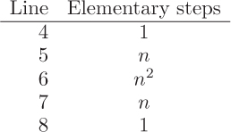
Like our previous algorithm, the maximum value in the table is n2, so our new algorithm is also a quadratic-time algorithm.
A more efficient algorithm
Reflection 8.28 Do you think it is possible to design a more efficient algorithm for this problem? If so, what part(s) of the algorithm would need to be made more efficient? Are there parts of the algorithm that are absolutely necessary and therefore cannot be made more efficient?
To find all of the duplicates in a list, it seems obvious that we need to look at every one of the n items in the list (using a for loop or some other kind of loop). Therefore, the time complexity of any algorithm for this problem must be at least n, or linear-time. But is a linear-time algorithm actually possible? Apart from the loop, the only significant component of the algorithm remaining is the linear search in line 6. Can the efficiency of this step be improved from linear time to something better?
Searching for data efficiently, as we do in a linear search, is a fundamental topic that is covered in depth in later computer science courses. There are a wide variety of innovative ways to store data to facilitate fast access, most of which are beyond the scope of an introductory book. However, we have already seen one alternative. Recall from Box 8.2 that a dictionary is cleverly implemented so that access can be considered a constant-time operation. So if we can store information about duplicates in a dictionary, we should be able to perform the search in line 6 in constant time!
The trick is to store the items that we have already seen as keys in a dictionary. In particular, when we append a value of item to the list of unique items, we also make item a new key in the dictionary. Then we can test whether we want to append each new value of item by checking whether item is already a key in seen. The new function with these changes follows.
def removeDuplicates3(data):
    """ (docstring omitted) """

    seen = { }
    unique = [ ]
    for item in data:
          if item not in seen:
              unique.append(item)
              seen[item] = True
    return unique
In our new function, we associate the value True with each key, but this is an arbitrary choice because we never actually use these values.
Since every statement in the body of the for loop is now one elementary step, the removeDuplicates3 function is a linear-time algorithm. As we saw in Figure 8.3, this makes a significant difference! Exercise 8.5.2 asks you to investigate this difference for yourself.
Exercises
8.5.1. Show how to modify each of the three functions we wrote so that they each instead return a list of only those items in data that have duplicates. For example, if data were [1, 2, 3, 1, 3, 1], the function should return the list [1, 3].
8.5.2. In this exercise, you will write a program that tests whether the linear-time removeDuplicates3 function really is faster than the first two versions that we wrote. First, write a function that creates a list of n random integers between 0 and n – 1 using a list accumulator and the random.randrange function. Then write another function that calls each of the three functions with such a list as the argument. Time how long each call takes using the time.time function, which returns the current time in elapsed seconds since a fixed “epoch” time (usually midnight on January 1, 1970). By calling time.time before and after each call, you can find the number of seconds that elapsed.
Repeat your experiment with n = 100, 1000, 10, 000, and 100, 000 (this will take a long time). Describe your results.
8.5.3. In a round-robin tournament, every player faces every other player exactly once, and the player with the most head-to-head wins is deemed the champion. The following partially written algorithm simulates a round-robin tournament. Assume that each of the steps expressed as a comment is one elementary step.
def roundRobin(players):
    # initialize all players' win counts to zero
    for player1 in players:
        for player2 in players:
            if player2 != player1:
                # player1 challenges player2
                # increment the win count of the winner
    # return the player with the most wins (or tie)
What is the asymptotic time complexity of this algorithm?
8.5.4. The nested loop in the previous function actually generates far too many contests. Not only does it create situations in which the two players are the same person, necessitating the if statement, it also considers every head-to-head contest twice. The illustration on the left below (a) shows all of the contests created by the nested for loop in the previous function in a four-player tournament.
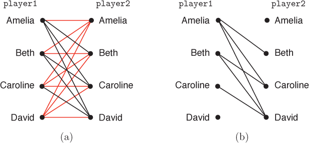
A line between two players represents the player on the left challenging the player on the right. Notice, for example, that Amelia challenges Caroline and Caroline challenges Amelia. Obviously, these are redundant, so we would like to avoid them. The red lines represent all of the unnecessary contests. The remaining contests that we need to consider are illustrated on the right side above (b).
- Let’s think about how we can design an algorithm to create just the contests we need. Imagine that we are iterating from top to bottom over the
playerslist on the left side of (b) above. Notice that each value ofplayer1on the left only challenges values ofplayer2on the right that come after it in the list. First, Amelia needs to challenge Beth, Caroline, and David. Then Beth only needs to challenge Caroline and David because Amelia challenged her in the previous round. Then Caroline only needs to challenge David because both Amelia and Beth already challenged her in previous rounds. Finally, when we get to David, everyone has already challenged him, so nothing more needs to be done.
Modify the nestedforloop in the previous exercise so that it implements this algorithm instead. - What is the asymptotic time complexity of your algorithm?
8.5.5. Suppose you have a list of projected daily stock prices, and you wish to find the best days to buy and sell the stock to maximize your profit. For example, if the list of daily stock prices was [3, 2, 1, 5, 3, 9, 2], you would want to buy on day 2 and sell on day 5, for a profit of $8 per share. Similar to the previous exercise, you need to check all possible pairs of days, such that the sell day is after the buy day. Write a function
profit(prices)
that returns a tuple containing the most profitable buy and sell days for the given list of prices. For example, for the list of daily prices above, your function should return (2, 5).
*8.6 LINEAR REGRESSION
Suppose you work in college admissions, and would like to determine how well various admissions data predict success in college. For example, if an applicant earned a 3.1 GPA in high school, is that a predictor of cumulative college GPA? Are SAT scores better or worse predictors?
Analyses such as these, looking for relationships between two (or more) variables, are called regression analyses. In a regression analysis, we would like to find a function or formula that accurately predicts the value of a dependent variable based on the value of an independent variable. In the college admissions problem, the independent variables are high school GPA and SAT scores, and the dependent variable is cumulative GPA in college. A regression analysis would choose one independent variable (e.g., high school GPA) and try to find a function that accurately predicts the value of one dependent variable (e.g., college GPA). Regression is a fundamental technique of data mining, which seeks to extract patterns and other meaningful information from large data sets.
The input to a regression problem is a data set consisting of n pairs of values. The first value in each pair is a value of the independent variable and the second value is the corresponding value of the dependent variable. For example, consider the following very small data set.
High school GPA |
College GPA |
|---|---|
3.1 |
2.8 |
3.8 |
3.7 |
3.4 |
3.2 |
We can also think of each row in the table, which represents one student, as an (x, y) point where x is the value of the independent variable and y is the value of the dependent variable.
The most common type of regression analysis is called linear regression. A linear regression finds a straight line that most closely approximates the relationship between the two variables. The most commonly used linear regression technique, called the least squares method, finds the line that minimizes the sum of the squares of the vertical distances between the line and our data points. This is represented graphically below.
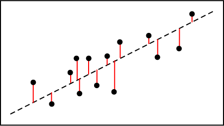
The red line segments in the figure represent the vertical distances between the points and the dashed line. This dashed line represents the line that results in the minimum total squared vertical distance for these points.
Mathematically, we are trying to find the line y = mx + b (with slope m and y-intercept b) for which
is the minimum. The x and y in this notation represent any one of the points (x, y) in our data set; (y – (mx + b)) represents the vertical distance between the height of (x, y) (given by y) and the height of the line at (x, y) (given by mx + b). The upper case Greek letter sigma (∑) means that we are taking the sum over all such points (x, y) in our data set.
To find the least squares line for a data set, we could test all of the possible lines, and choose the one with the minimum total squared distance. However, since there are an infinite number of such lines, this “brute force” approach would take a very long time. Fortunately, the least squares line can be found exactly using calculus. The slope m of this line is given by
and the y-intercept b is given by
Although the notation is these formulas may look imposing, the quantities are really quite simple:
n is the number of points
Σx is the sum of the x coordinates of all of the points (x, y)
Σy is the sum of the y coordinates of all of the points (x, y)
Σ(xy) is the sum of x times y for all of the points (x, y)
Σ(x2) is the sum of the squares of the x coordinates of all of the points (x, y)
For example, suppose we had only three points: (5, 4), (3, 2), and (8, 3). Then
Σx = 5 + 3 + 8 = 16
Σy = 4 + 2 + 3 = 9
Σ(xy) = (5 · 4) + (3 · 2) + (8 · 3) = 20 + 6 + 24 = 50
Σ(x2) = 52 + 32 + 82 = 25 + 9 + 64 = 98
Therefore,
and
Plugging in these values, we find that the formula for the least squares line is
which is plotted below.
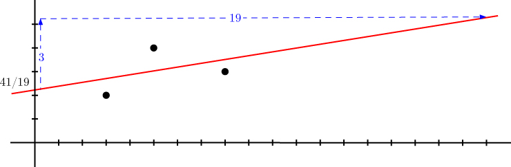
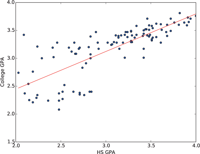
Figure 8.5 Scatter plot showing high school GPA and corresponding cumulative college GPA with regression line.
Given these formulas, it is fairly easy to write a function linearRegression to find the least squares regression line. Suppose the function takes as parameters a list of x coordinates named x and a list of y coordinates named y (just like the matplotlib plot function). The x coordinates are values of the independent variable and the y coordinates are the values of the dependent variable. Then we can use four accumulator variables to store the four sums above. For example, ∑ x can be computed with
n = len(x)             # number of points
sumx = 0               # sum of x coordinates
for index in range(n):
    sumx = sumx + x[index]
Once all of the sums are computed, m and b can be computed and returned with
return m, b
Exercise 8.6.1 asks you to complete the implementation of this function.
Once we have a function that performs linear regression, it is fairly simple to plot a set of points with the regression line:
def plotRegression(x, y, xLabel, yLabel):
    """Plot points in x and y with a linear regression line.

    Parameters:
        x: a list   of x values (independent variable)
        y: a list   of y values (dependent variable)
        xLabel: a   string to label the x axis
        yLabel: a   string to label the y axis

    Return value: None
    """

    pyplot.scatter(x, y)
    m, b = linearRegression(x, y)
    minX = min(x)
    maxX = max(x)
    pyplot.plot([minX, maxX], [m * minX + b, m * maxX + b], color = 'red')
    pyplot.xlabel(xLabel)
    pyplot.ylabel(yLabel)
    pyplot.show()
Returning to our college admissions problem, suppose the high school GPA values are in a list named hsGPA and the college GPA values are in a list named collegeGPA. Then we can get our regression line by calling
plotRegression(hsGPA, collegeGPA, 'HS GPA', 'College GPA')
An example plot based on real data is shown in Figure 8.5.
Reflection 8.29 What can you discern from this plot? Does high school GPA do a good job of predicting college GPA?
In the exercises below, and in Project 8.4, you will have the opportunity to investigate this problem in more detail. Projects 8.3 and 8.5 also use linear regression to approximate the demand curve for an economics problem and predict flood levels on the Snake River, respectively.
Exercises
linearRegression(x, y)
The function should return the slope and y-intercept of the least squares regression line for the points whose x and y coordinates are stored in the lists x and y, respectively. (Your function should use only one loop.)
8.6.2. The table below lists the homework and exam scores for a class (one row per student). Write a program that uses the completed linearRegression function from the previous exercise and the plotRegression function above to plot a linear regression line for this data.
8.6.3. On the book web site, you will find a CSV data file named sat.csv that contains GPA and SAT data for 105 students. Write a function
readData(filename)
that reads the data from this file and returns a tuple of two lists containing the data in the first and fourth columns of the file (high school GPAs and college GPAs). Then use the plotRegression function (which will call your completed linearRegression function from the previous exercise) to plot this data with a linear regression line to determine whether there is a correlation between high school GPA and college GPA. (Your plot should look like Figure 8.5.)
8.6.4. A standard way to measure how well a regression line fits a set of data is to compute the coefficient of determination, often called the R2 coefficient, of the regression line. R2 is defined to be
where S and T are defined as follows:
S = ∑ (y – (mx + b))2
For example, the example with three points in the text: (5, 4), (3, 2), and (8, 3).
We saw that these points have regression line
(So m = 3/14 and b = 13/7.) Then
y¯=(4+2+3)/3=3 T=Σ(y−y¯)2=(4−3)2+(2−3)2+(3−3)2=2 S = Σ(y – (mx + b))2 = (4 – 41/14)2 + (2 – 5/2)2 + (3 – 25/7)2 = 169/98
R2 = 1 – (169/98)/2 = 1 – 169/196 = 27/196 ≈ 0.137755
The R2 coefficient is always between 0 and 1, with values closer to 1 indicating a better fit.
Write a function
rSquared(x, y, m, b)
that returns the R2 coefficient for the set of points whose x and y coordinates are stored in the lists x and y, respectively. The third and fourth parameters are the slope and y-intercept of the regression line for the set of points. For example, to apply your function to the example above, we would call
rSquared([5, 3, 8], [4, 2, 3], 3/14, 13/7)
8.6.5. An alternative linear regression method, called a Deming regression finds the line that minimizes the squares of the perpendicular distances between the points and the line rather than the vertical distances. While the traditional least squares method accounts only for errors in the y values, this technique accounts for errors in both x and y. The slope and y-intercept of the line found by this method are2
and
where
x¯ = (1/n) ∑ x, the mean of the x coordinates of all of the points (x, y)y¯ = (1/n) ∑ y, the mean of the y coordinates of all of the points (x, y)sxx = (1/(n – 1)) ∑(x –
x¯ )2syy = (1/(n – 1)) ∑(y –
y¯ )2sxy = (1/(n – 1)) ∑(x –
x¯ ) (y –y¯ )
Write a function
linearRegressionDeming(x, y)
that computes these values of m and b. Test your function by using it in the plotRegression function above.
*8.7 DATA CLUSTERING
In some large data sets, we are interested in discovering groups of items that are similar in some way. For example, suppose we are trying to determine whether a suite of test results is indicative of a malignant tumor. If we have these test results for a large number of patients, together with information about whether each patient has been diagnosed with a malignant tumor, then we can test whether clusters of similar test results correspond uniformly to the same diagnosis. If they do, the clustering is evidence that the tests can be used to test for malignancy, and the clusters give insights into the range of results that correspond to that diagnosis. Because data clustering can result in deep insights like this, it is another fundamental technique used in data mining.
Algorithms that cluster items according to their similarity are easiest to understand initially with two-dimensional data (e.g., longitude and latitude) that can be represented visually. Therefore, before you tackle the tumor diagnosis problem (as an exercise), we will look at a data set containing the geographic locations of vehicular collisions in New York City.3
The clustering problem turns out to be very difficult, and there are no known efficient algorithms that solve it exactly. Instead, people use heuristics. A heuristic is an algorithm that does not necessarily give the best answer, but tends to work well in practice. Colloquially, you might think of a heuristic as a “good rule of thumb.” We will discuss a common clustering heuristic known as k-means clustering. In k-means clustering, the data is partitioned into k clusters, and each cluster has an associated centroid, defined to be the mean of the points in the cluster. The k-means clustering heuristic consists of a number of iterations in which each point is (re)assigned to the cluster of the closest centroid, and then the centroids of each cluster are recomputed based on their potentially new membership.
Defining similarity
Similarity among items in a data set can be defined in a variety of ways; here we will define similarity simply in terms of normal Euclidean distance. If each item in our data set has m numerical attributes, then we can think of these attributes as a point in m-dimensional space. Given two m-dimensional points p and q, we can find the distance between them using the formula
In Python, we can represent each point as a list of m numbers. For example, each of the following three lists might represent six test results (m = 6) for one patient:
p1 = [85, 92, 45, 27, 31, 0.0]
p2 = [85, 64, 59, 32, 23, 0.0]
p3 = [86, 54, 33, 16, 54, 0.0]
But since we are not going to need to change any element of a point once we read it from a data file, a better alternative is to store each point in a tuple, as follows:
Box 8.4: Privacy in the Age of Big Data
Companies collect (and buy) a lot of data about their customers, including demographics (age, address, marital status), education, financial and credit history, buying habits, and web browsing behavior. They then mine this data, using techniques like clustering, to learn more about customers so they can target customers with advertising that is more likely to lead to sales. But when does this practice lead to unacceptable breaches of privacy? For example, a recent article explained how a major retailer is able to figure out when a woman is pregnant before her family does.
When companies store this data online, it also becomes vulnerable to unauthorized access by hackers. In recent years, there have been several high-profile incidents of retail, government, and financial data breaches. As our medical records also begin to migrate online, more people are taking notice of the risks involved in storing “big data.”
So as you continue to work with data, remember to always balance the reward with the inherent risk. Just because we can do something doesn’t mean that we should do it.
p1 = (85, 92, 45, 27, 31, 0.0)
p2 = (85, 64, 59, 32, 23, 0.0)
p3 = (86, 54, 33, 16, 54, 0.0)
To find the distance between tuples p1 and p2, we can compute
and to find the distance between tuples p1 and p3, we can compute
Because the distance between p1 and p2 is less than the distance between p1 and p3, we consider the results for patient p1 to be more similar to the results for patient p2 than to the results for patient p3.
Reflection 8.30 What is the distance between tuples p2 and p3? Which patient’s results are more similar to each of p2 and p3?
A k-means clustering example
To illustrate in more detail how the heuristic works, consider the following small set of six points, and suppose we want to group them into k = 2 clusters. The lower left corner of the rectangle has coordinates (0, 0) and each square is one unit on a side. So our six points have coordinates (0.5, 5), (1.75, 5.75), (3.5, 2), (4, 3.5), (5, 2), and (7, 1).
We begin by randomly choosing k = 2 of our points to be the initial centroids. In the figure below, we chose one centroid to be the red point at (0.5, 5) and the other centroid to be the blue point at (7, 1).
In the first iteration of the heuristic, for every point, we compute the distance between the point and each of the two centroids, represented by the dashed line segments. We assign each point to a cluster associated with the centroid to which it is closest. In this example, the three points circled in red below are closest to the red centroid and the three points circled in blue below are closest to the blue centroid.
Once every point is assigned to a cluster, we compute a new centroid for each cluster, defined to be the mean of all the points in the cluster. In our example, the x and y coordinates of the new centroid of the red cluster are (0.5 + 1.75 + 4)/3 = 25/12 ≈ 2.08 and (5 + 5.75 + 3.5)/3 = 4.75. The x and y coordinates of the new centroid of the blue cluster are (3.5 + 5 + 7)/3 = 31/6 ≈ 5.17 and (2 + 2 + 1)/3 = 5/3 ≈ 1.67. These are the new red and blue points shown below.
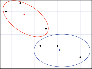
In the second iteration of the heuristic, we once again compute the closest centroid for each point. As illustrated below, the point at (4, 3.5) is now grouped with the lower right points because it is closer to the blue centroid than to the red centroid (distance ((2.08, 4.75), (4, 3.5)) ≈ 2.29 and distance((5.17, 1.67), (4, 3.5)) ≈ 2.17).

Next, we once again compute new centroids. The x and y coordinates of the new centroid of the red cluster are (0.5 + 1.75)/2 = 1.125 and (5 + 5.75)/2 = 5.375. The x and y coordinates of the new centroid of the blue cluster are (3.5 + 4 + 5 + 7)/4 = 4.875 and (1 + 2 + 2 + 3.5)/4 = 2.125. These new centroids are shown below.
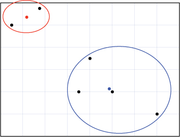
In the third iteration, when we find the closest centroid for each point, we find that nothing changes. Therefore, these clusters are the final ones chosen by the heuristic.
Implementing k-means clustering
To implement this heuristic in Python, we define the function named kmeans below with three parameters: a list of tuples named data, the number of clusters k, and iterations, the number of iterations in the heuristic. If we were calling the function with the points in the previous example, then data would be assigned the list
[(0.5, 5), (1.75, 5.75), (3.5, 2), (4, 3.5), (5, 2), (7, 1)]
def kmeans(data, k, iterations):
    """Cluster data into k clusters using the given number of
       iterations of the k-means clustering algorithm.

    Parameters:
        data: a list of points
        k: the number of desired clusters
        iterations: the number of iterations of the algorithm

    Return value:
        a tuple containing the list of clusters and the list
        of centroids; each cluster is represented by a list
        of indices of the points assigned to that cluster
    """

    n = len(data)
    centroids = random.sample(data, k)  # k initial centroids

    for step in range(iterations):
The function begins by using the sample function from the random module to choose k random tuples from data to be the initial centroids, assigned to the variable named centroids. The remainder of the function consists of iterations passes over the list of points controlled by the for loop above.
Next, within the loop, we first create a list of k empty lists, one for each cluster. For example, if k was 4 then, after the following three lines, clusters would be assigned the list [[ ], [ ], [ ], [ ]].
clusters = []
for i in range(k):
    clusters.append([])
The first empty list, clusters[0], will be used to hold the indices of the points in the cluster associated with centroids[0]; the second empty list, clusters[1], will be used to hold the indices of the points in the cluster associated with centroids[1]; and so on. Some care has to be taken to create this list of lists; clusters = [[]] * k will not work. Exercise 8.7.6 asks you to investigate this further.
Next, we iterate over the indices of the points in data. In each iteration, we need to find the centroid that is closest to the point data[dataIndex].
for dataIndex in range(n):
    minIndex = 0
    for clustIndex in range(1, k):
        dist = distance(centroids[clustIndex], data[dataIndex])
        if dist < distance(centroids[minIndex], data[dataIndex]):
            minIndex = clustIndex
    clusters[minIndex].append(dataIndex)
The inner for loop above is essentially the same algorithm that we used in Section 8.1 to find the minimum value in a list. The difference here is that we need to find the index of the centroid with the minimum distance to data[dataIndex]. (We leave writing this distance function as Exercise 8.7.1.) Therefore, we maintain the index of the closest centroid in the variable named minIndex. Once we have found the final value of minIndex, we append dataIndex to the list of indices assigned to the cluster with index minIndex.
After we have assigned all of the points to a cluster, we compute each new centroid with a function named centroid. We leave writing this function as Exercise 8.7.2.
for clustIndex in range(k):
    centroids[clustIndex] = centroid(clusters[clustIndex], data)
Finally, once the outer for loop finishes, we return a tuple containing the list of clusters and the list of centroids.
return (clusters, centroids)
The complete function is reproduced below:
def kmeans(data, k, iterations):
    """ (docstring omitted) """

    n = len(data)
    centroids = random.sample(data, k)

    for step in range(iterations):
        clusters = []
        for i in range(k):
            clusters.append([])

        for dataIndex in range(n):
            minIndex = 0
            for clustIndex in range(1, k):
                dist = distance(centroids[clustIndex], data[dataIndex])
                if dist < distance(centroids[minIndex], data[dataIndex]):
                    minIndex = clustIndex
            clusters[minIndex].append(dataIndex)

        for clustIndex in range(k):
            centroids[clustIndex] = centroid(clusters[clustIndex], data)

    return (clusters, centroids)
Locating bicycle safety programs
Suppose that, in response to an increase in the number of vehicular accidents in New York City involving cyclists, we want to find the best locations to establish a limited number of bicycle safety programs. To do the most good, we would like to centrally locate these programs in areas containing the most cycling injuries. In other words, we want to locate safety programs at the centroids of clusters of accidents.
We can use the k-means clustering heuristic to find these centroids. First, we need to read the necessary attributes from a data file containing the accident information. This data file,4 which is available on the book web site, is tab-separated and contains a row for each of 7,642 collisions involving bicycles between August, 2011 and August, 2013 in all five boroughs of New York City. Associated with each collision are 68 attributes that include information about the location, injuries, and whether pedestrians or cyclists were involved. The first few rows of the data file look like this (with triangles representing tab characters):
borocode⊳precinct⊳year⊳month⊳lon⊳lat⊳street1⊳street2⊳collisions⊳...
3⊳60⊳2011⊳8⊳-73.987424⊳40.58539⊳CROPSEY AVENUE⊳SHORE PARKWAY⊳4⊳...
3⊳60⊳2011⊳8⊳-73.98584⊳40.576503⊳MERMAID AVENUE⊳WEST 19 STREET⊳2⊳...
3⊳60⊳2011⊳8⊳-73.983088⊳40.579161⊳NEPTUNE AVENUE⊳WEST 15 STREET⊳2⊳...
3⊳60⊳2011⊳8⊳-73.986609⊳40.574894⊳SURF AVENUE⊳WEST 20 STREET⊳1⊳...
3⊳61⊳2011⊳8⊳-73.955477⊳40.598939⊳AVENUE U⊳EAST 16 STREET⊳2⊳...
For our clustering algorithm, we will need a list of accident locations as (longitude, latitude) tuples. To limit the data in our analysis, we will extract the locations of only those accidents that occurred in Manhattan (borocode 1) during 2012. The function to accomplish this is very similar to what we have done previously.
def readFile(filename):
    """Read locations of 2012 bicycle accidents in Manhattan
       into a list of tuples.

     Parameter:
         filename: the name of the data file

     Return value: a list of (longitude, latitude) tuples
     """

     inputFile = open(filename, 'r', encoding = 'utf-8')
     header = inputFile.readline()
     data = [ ]
     for line in inputFile:
         row = line.split('	')
         borough = int(row[0])
         year = int(row[2])
         if (borough == 1) and (year == 2012):
             longitude = float(row[4])
             latitude = float(row[5])
             data.append( (longitude, latitude) )
     inputFile.close()
     return data
Once we have the data as a list of tuples, we can call the kmeans function to find the clusters and centroids. If we had enough funding for six bicycle safety programs, we would call the function with k = 6 as follows:
data = readFile('collisions_cyclists.txt')
(clusters, centroids) = kmeans(data, 6, 100)
To visualize the clusters, we can plot the points with matplotlib, with each cluster in a different color and centroids represented by stars. The following plotClusters function does just this. The result is shown in Figure 8.6.
import matplotlib.pyplot as pyplot

def plotClusters(clusters, data, centroids):
    """Plot clusters and centroids in unique colors.

     Parameters:
         clusters: a list of k lists of data indices
         data: a list of points
         centroids: a list of k centroid points

     Return value: None
     """

Figure 8.6 Six clusters of bicycle accidents in Manhattan with the centroid for each shown as a star.
    colors = ['blue', 'red', 'yellow', 'green', 'purple', 'orange']
    for clustIndex in range(len(clusters)):   # plot clusters of points
        x = []
        y = []
        for dataIndex in clusters[clustIndex]:
            x.append(data[dataIndex][0])
            y.append(data[dataIndex][1])
        pyplot.scatter(x, y, 10, color = colors[clustIndex])

    x = []
    y = []
    for centroid in centroids:    # plot centroids
        x.append(centroid[0])
        y.append(centroid[1])
    pyplot.scatter(x, y, 200, marker = '*', color = 'black')
    pyplot.show()
In Exercise 8.7.3, we ask you to combine the kmeans, readFile, and plotClusters functions into a complete program that produces the plot in Figure 8.6.
Reflection 8.31 If you look at the “map” in Figure 8.6, you will notice that the orientation of Manhattan appears to be more east-west than it is in reality. Do you know why?
In addition to completing this program, Exercise 8.7.4 asks you to apply k-means clustering to the tumor diagnosis problem that we discussed at the beginning of the chapter.
Exercises
distance(p, q)
that returns the Euclidean distance between k-dimensional points p and q, each of which is represented by a tuple with length k.
centroid(cluster, data)
that is needed by the kmeans function. The function should compute the centroid of the given cluster, which is a list of indices of points in data. Remember that the points in data can be of any length, and the centroid that the function returns must be a tuple of the same length. It will probably be most convenient to build up the centroid in a list and then convert it to a tuple using the tuple function. If the cluster is empty, then return a randomly chosen point from data with random.choice(data).
8.7.3. Combine the distance and centroid functions that you wrote in the previous two exercises with the kmeans, readFile, and plotClusters functions to create a complete program (with a main function) that produces the plot in Figure 8.6. The data file, collisions_cyclists.txt, is available on the book web site.
8.7.4. In this exercise, you will apply k-means clustering to the tumor diagnosis problem from the beginning of this section, using a data set of breast cancer biopsy results. This data set, available on the book web site, contains nine test results for each of 683 individuals.5 The first few lines of the comma-separated data set look like:
1000025,5,1,1,1,2,1,3,1,1,2
1002945,5,4,4,5,7,10,3,2,1,2
1015425,3,1,1,1,2,2,3,1,1,2
1016277,6,8,8,1,3,4,3,7,1,2
1017023,4,1,1,3,2,1,3,1,1,2
1017122,8,10,10,8,7,10,9,7,1,4
  .
  .
  .
The first number in each column is a unique sample number and the last number in each column is either 2 or 4, where 2 means “benign” and 4 means “malignant.”
Of the 683 samples in the data set, 444 were diagnosed as benign and 239 were diagnosed as malignant. The nine numbers on each line between the sample number and the diagnosis are test result values that have been normalized to a 1–10 scale. (There is additional information accompanying the data on the book’s web site.)
The first step is to write a function
readFile(filename)
that reads this data and returns two lists, one of test results and the other of diagnoses. The test results will be in a list of 9-element tuples and the diagnosis values will be a list of integers that are in the same order as the test results.
Next, write a program, with the following main function, that clusters the data into k = 2 groups. If one of these two groups contains predominantly benign samples and the other contains predominantly malignant samples, then we can conclude that these test results can effectively discriminate between malignant and benign tumors.
def main():
    data, diagnosis = readFile('breast-cancer-wisconsin.csv')
    clusters, centroids = kmeans(data, 2, 10)
    for clustIndex in range(2):
        count = {2: 0, 4: 0}
        for index in clusters[clustIndex]:
            count[diagnosis[index]] = count[diagnosis[index]] + 1
        print('Cluster', clustIndex)
        print(' benign:', count[2], 'malignant:', count[4])
To complete the program, you will need to incorporate the distance and centroid functions from Exercises 8.7.1 and 8.7.2, the kmeans function, and your readFile function. The data file, breast-cancer-wisconsin.csv, is available on the book web site. Describe the results.
8.7.5. Given data on 100 customers’ torso length and chest measurements, use k-means clustering to cluster the customers into three groups: S, M, and L. (Later, you can use this information to design appropriately sized t-shirts.) You can find a list of measurements on the book web site.
8.7.6. In the kmeans function, we needed to create a new list of empty clusters at the beginning of each iteration. To create this list, we did the following:
clusters = []
for i in range(k):
    clusters.append([])
Alternatively, we could have created a list of lists using the * repetition operator like this:
clusters = [[]] * k
However, this will not work correctly, as evidenced by the following:
>>> clusters = [[]] * 5
>>> clusters
[[], [], [], [], []]
>>> clusters[2].append(4)
>>> clusters
[[4], [4], [4], [4], [4]]
What is going on here?
8.7.7. Modify the kmeans function so that it does not need to take the number of iterations as a parameter. Instead, the function should iterate until the list of clusters stops changing. In other words, the loop should iterate while the list of clusters generated in an iteration is not the same as the list of clusters from the previous iteration.
8.8 SUMMARY
Those who know how to manipulate and extract meaning from data will be well positioned as the decision makers of the future. Algorithmically, the simplest way to store data is in a list. We developed algorithms to summarize the contents of a list with various descriptive statistics, modify the contents of lists, and create histograms describing the frequency of values in a list. The beauty of these techniques is that they can be used with a wide variety of data types and applications. But before any of them can be used on real data, the data must be read from its source and wrangled into a usable form. To this end, we also discussed basic methods for reading and formatting tabular data both from local files and from the web.
In later sections, we went beyond simply describing data sets to data mining techniques that can make predictions from them. Linear regression seeks a linear pattern in data and then uses this pattern to predict missing data points. The k-means clustering algorithm partitions data into clusters of like elements to elicit hidden relationships.
Algorithms that manipulate lists can quickly become much more complicated than what we have seen previously, and therefore paying attention to their time complexity is important. To illustrate, we worked through a sequence of three increasingly more elegant and more efficient algorithms for removing duplicates from a list. In the end, we saw that the additional time taken to think through a problem carefully and reduce its time complexity can pay dividends.
8.9 FURTHER DISCOVERY
Sherlock Holmes was an early data scientist, always insisting on fact-based theories (and not vice versa). The chapter epigraph is from Sir Arthur Conan Doyle’s short story, The Adventure of the Copper Beeches [11].
A good resource for current data-related news is the “data journalism” web site FiveThirtyEight at http://fivethirtyeight.com. If you are interested in learning more about the emerging field of data science, one resource is Doing Data Science by Rachel Schutt and Cathy O’Neil [49].
The article referenced in Box 8.4 is from The New York Times [12]. The nonprofit Electronic Frontier Foundation (EFF), founded in 1990, works at the forefront of issues of digital privacy and free speech. To learn more about contemporary privacy issues, visit its website at http://www.eff.org. For more about ethical issues in computing in general, we recommend Computer Ethics by Deborah Johnson and Keith Miller [21].
8.10 PROJECTS
Project 8.1 Climate change
The causes and consequences of global warming are of intense interest. The consensus of the global scientific community is that the primary cause of global warming is an increased concentration of “greenhouse gasses,” primarily carbon dioxide (CO2) in the atmosphere. In addition, it is widely believed that human activity is the cause of this increase, and that it will continue into the future if we do not limit what we emit into the atmosphere.
To understand the causes of global warming, and to determine whether the increase in CO2 is natural or human-induced, scientists have reconstructed ancient climate patterns by analyzing the composition of deep ocean sediment core samples. In a core sample, the older sediment is lower and the younger sediment is higher. These core samples contain the remains of ancient bottom-dwelling organisms called foraminifera that grew shells made of calcium carbonate (CaCO3).
Virtually all of the oxygen in these calcium carbonate shells exists as one of two stable isotopes: oxygen-16 (16O) and oxygen-18 (18O). Oxygen-16 is, by far, the most common oxygen isotope in our atmosphere and seawater at about 99.76% and oxygen-18 is the second most common at about 0.2%. The fraction of oxygen-18 incorporated into the calcium carbonate shells of marine animals depends upon the temperature of the seawater. Given the same seawater composition, colder temperatures will result in a higher concentration of oxygen-18 being incorporated into the shells. Therefore, by analyzing the ratio of oxygen-18 to oxygen-16 in an ancient shell, scientists can deduce the temperature of the water at the time the shell formed. This ratio is denoted δ18O; higher values of δ18O represent lower temperatures.
Similarly, it is possible to measure the relative amounts of carbon isotopes in calcium carbonate. Carbon can exist as one of two stable isotopes: carbon-12 (12C) and carbon-13 (13C). (Recall from Section 4.4 that carbon-14 (14C) is radioactive and used for radiocarbon dating.) δ13C is a measure of the ratio of carbon-13 to carbon-12. The value of δ13C can decrease, for example, if there were a sudden injection of 12C-rich (i.e., 13C-depleted) carbon. Such an event would likely cause an increase in warming due to the increase in greenhouse gasses.
In this project, we will examine a large data set [60] containing over 17,000 δ18O and δ13C measurements from deep ocean sediment core samples, representing conditions over a period of about 65 million years. From this data, we will be able to visualize deep-sea temperature patterns over time (based on the δ18O measurements) and the accompanying values of δ13C. We can try to answer two questions with this data. First, is there a correspondence between changes in carbon output and changes in temperature? Second, are recent levels of carbon in the atmosphere and ocean "natural," based on what has happened in the past?
Part 1: Read and plot the data
First, download the file named 2008CompilationData.csv from the book web site.6 Examine the file and write a function that creates four parallel lists containing information about δ18O and δ13C readings: one list containing the δ18O measurements, one list containing the δ13C measurements, one list containing the sites of the measurements, and a fourth list containing the ages of the measurements. (Note that the Age (ma) column represents the ages of the samples in millions of years.) If a row is missing either the δ18O value or the δ13C value, do not include that row in your lists.
Using matplotlib, create scatter plots of the δ18O and δ13C measurements separately with respect to time (we will use the list of sites later). Be sure to appropriately label your axes. Because there is a lot of data here, your plots will be clearer if you make the dots small by passing s = 1 into the scatter function. To create two plots in separate windows, precede the first plot with pyplot.figure(1) and precede the second plot with pyplot.figure(2):
pyplot.figure(1)

# plot d18O data here

pyplot.figure(2)

# plot d13C data here

pyplot.show() # after all the figures
Part 2: Smooth and plot the data
Inconsistencies in sampling, and local environmental variation, result in relatively noisy plots, but this can be fixed with a smoothing function that computes means in a window moving over the data. This is precisely the algorithm we developed back in Section 1.3 (and Exercise 8.2.14). Write a function that implements this smoothing algorithm, and use it to create three new lists — for δ18O, δ13C, and the ages — that are smoothed over a window of length 5.
To compare the oxygen and carbon isotope readings, it will be convenient to create two plots, one over the other, in the same window. We can do this with the matplotlib subplot function:
pyplot.figure(3)
pyplot.subplot(2, 1, 1) # arguments are (rows, columns, subplot #)

# plot d18O here

pyplot.subplot(2, 1, 2)

# plot d13C here
Part 3: The PETM
Looking at your smoothed data, you should now clearly see a spike in temperature (i.e., rapid decrease in δ18O) around 55 ma. This event is known as the Palaeocene-Eocene Thermal Maximum (PETM), during which deep-sea temperatures rose 5° to 6° Celsius in fewer than 10,000 years!
To investigate further what might have happened during this time, let’s “zoom in” on this period using data from only a few sites. Create three new lists, one of ages and the other two of measurements, that contain data only for ages between 53 and 57 ma and only for sites 527, 690, and 865. Sites 527 and 690 are in the South Atlantic Ocean, and site 865 is in the Western Pacific Ocean. (Try using list comprehensions to create the three lists.)
Plot this data in the same format as above, using two subplots.
Question 8.1.1 What do you notice? What do your plots imply about the relationship between carbon and temperature?
Part 4: Recent history
To gain insight into what “natural” CO2 levels have looked like in our more recent history, we can consult another data set, this time measuring the CO2 concentrations in air bubbles trapped inside ancient Antarctic ice [39]. Download this tab-separated data file from the book web site, and write code to extract the data into two parallel lists — a list of ages and a list of corresponding CO2 concentrations. The CO2 concentrations are measured in parts per million by volume (ppmv) and the ages are in years.
Next, plot your data. You should notice four distinct, stable cycles, each representing a glacial period followed by an interglacial period. To view the temperature patterns during the same period, we can plot the most recent 420,000 years of our δ18O readings. To do so, create two new parallel lists — one containing the δ18O readings from sites 607, 659, and 849 for the last 420,000 years, and the other containing the corresponding ages. Arrange a plot of this data and your plot of CO2 concentrations in two subplots, as before.
Question 8.1.2 What do you notice? What is the maximum CO2 concentration during this period?
Part 5: Very recent history
In 1958, geochemist Charles David Keeling began measuring atmospheric CO2 concentrations at the Mauna Loa Observatory (MLO) on the big island of Hawaii. These measurements have continued for the past 50 years, and are now known as the Keeling curve. Available on the book web site (and at http://scrippsco2.ucsd.edu/data/mlo.html) is a CSV data file containing weekly CO2 concentration readings (in ppmv) since 1958. Read this data into two parallel lists, one containing the CO2 concentration readings and the other containing the dates of the readings. Notice that the file contains a long header in which each line starts with a quotation mark. To read past this header, you can use the following while loop:
line = inputFile.readline() # inputFile is your file object name
while line[0] == '"':
    line = inputFile.readline()
Each of the dates in the file is a string in YYYY-MM-DD format. To convert each of these date strings to a fractional year (e.g., 2013-07-01 would be 2013.5), we can use the following formula:
year = float(date[:4]) + (float(date[5:7]) + float(date[8:10])/31) / 12
Next, plot the data.
Question 8.1.3 How do these levels compare with the maximum level from the previous 420,000 years? Is your plot consistent with the pattern of “natural” CO2 concentrations from the previous 420,000 years? Based on these results, what conclusions can we draw about the human impact on atmospheric CO2 concentrations?
Project 8.2 Does education influence unemployment?
Conventional wisdom dictates that those with more education have an easier time finding a job. In this project, we will investigate this claim by analyzing 2012 data from the U.S. Census Bureau.7
Part 1: Get the data
Download the data file from the book web site and look at it in a text editor. You will notice that it is a tab-separated file with one line per U.S. metropolitan area. In each line are 60 columns containing population data broken down by educational attainment and employment status. There are four educational attainment categories: less than high school graduate (i.e., no high school diploma), high school graduate, some college or associate’s degree, and college graduate.
Economists typically define unemployment in terms of the “labor force,” people who are available for employment at any given time, whether or not they are actually employed. So we will define the unemployment rate to be the fraction of the (civilian) labor force that is unemployed. To compute the unemployment rate for each category of educational attainment, we will need data from the following ten columns of the file:
Column index |
Contents |
|---|---|
2 |
Name of metropolitan area |
3 |
Total population of metropolitan area |
11 |
No high school diploma, total in civilian labor force |
15 |
No high school diploma, unemployed in civilian labor force |
25 |
High school graduate, total in civilian labor force |
29 |
High school graduate, unemployed in civilian labor force |
39 |
Some college, total in civilian labor force |
43 |
Some college, unemployed in civilian labor force |
53 |
College graduate, total in civilian labor force |
57 |
College graduate, unemployed in civilian labor force |
Read this data from the file and store it in six lists that contain the names of the metropolitan areas, the total populations, and the unemployment rates for each of the four educational attainment categories. Each unemployment rate should be stored as a floating point value between 0 and 100, rounded to one decimal point. For example, 0.123456 should be stored as 12.3.
Next, use four calls to the matplotlib plot function to plot the unemployment rate data in a single figure with the metropolitan areas on the x-axis, and the unemployment rates for each educational attainment category on the y-axis. Be sure to label each plot and display a legend. You can place the names of the metropolitan areas on the x-axis with the xticks function:
pyplot.xticks(range(len(names)), names, rotation = 270, fontsize = 'small')
The first argument is the locations of the ticks on the x-axis, the second argument is a list of labels to place at those ticks, and the third and fourth arguments optionally rotate the text and change its size.
Part 2: Filter the data
Your plot should show data for 366 metropolitan areas. To make trends easier to discern, let’s narrow the data down to the most populous areas. Create six new lists that contain the same data as the original six lists, but for only the thirty most populous metropolitan areas. Be sure to maintain the correct correspondence between values in the six lists. Generate the same plot as above, but for your six shorter lists.
Part 3: Analysis
Write a program to answer each of the following questions.
Question 8.2.1 In which of the 30 metropolitan areas is the unemployment rate higher for HS graduates than for those without a HS diploma?
Question 8.2.2 Which of the 30 metropolitan areas have the highest and lowest unemployment rates for each of the four categories of educational attainment? Use a single loop to compute all of the answers, and do not use the built-in min and max functions.
Question 8.2.3 Which of the 30 metropolitan areas has the largest difference between the unemployment rates of college graduates and those with only a high school diploma? What is this difference?
Question 8.2.4 Print a formatted table that ranks the 30 metropolitan areas by the unemployment rates of their college graduates. (Hint: use a dictionary.)
Project 8.3 Maximizing profit
Part 4 of this project assumes that you have read Section 8.6.
Suppose you are opening a new coffee bar, and need to decide how to price each shot of espresso. If you price your espresso too high, no customers will buy from you. On the other hand, if you price your espresso too low, you will not make enough money to sustain your business.
Part 1: Poll customers
To determine the most profitable price for espresso, you poll 1,000 potential daily customers, asking for the maximum price they would be willing to pay for a shot of espresso at your coffee bar. To simulate these potential customers, write a function
randCustomers(n)
that returns a list of n normally distributed prices with mean $4.00 and standard deviation $1.50. Use this function to generate a list of maximum prices for your 1,000 potential customers, and display of histogram of these maximum prices.
Part 2: Compute sales
Next, based on this information, you want to know how many customers would buy espresso from you at any given price. Write a function
sales(customers, price)
that returns the number of customers willing to buy espresso if it were priced at the given price. The first parameter customers is a list containing the maximum price that each customer is willing to pay. Then write another function
plotDemand(customers, lowPrice, highPrice, step)
that uses your sales function to plot a demand curve. A demand curve has price on the x-axis and the quantity of sales on the y-axis. The prices on the x-axis should run from lowPrice to highPrice in increments of step. Use this function to draw a demand curve for prices from free to $8.00, in increments of a quarter.
Part 3: Compute profits
Suppose one pound (454 g) of roasted coffee beans costs you $10.00 and you use 8 g of coffee per shot of espresso. Each “to go” cup costs you $0.05 and you estimate that half of your customers will need “to go” cups. You also estimate that you have about $500 of fixed costs (wages, utilities, etc.) for each day you are open. Write a function
profits(customers, lowPrice, highPrice, step, perCost, fixedCost)
that plots your profit at each price. Your function should return the maximum profit, the price at which the maximum profit is attained, and the number of customers who buy espresso at that price. Do not use the built-in min and max functions.
Question 8.3.1 How should you price a shot of espresso to maximize your profit? At this price, how much profit do you expect each day? How many customers should you expect each day?
*Part 4: Find the demand function
If you have not already done so, implement the linear regression function discussed in Section 8.6. (See Exercise 8.6.1.) Then use linear regression on the data in your demand plot in Part 2 to find the linear function that best approximates the demand. This is called the demand function. Linear demand functions usually have the form
where Q is the quantity sold and P is the price. Modify your plotDemand function so that it computes the regression line and plots it with the demand curve.
Question 8.3.2 What is the linear demand function that best approximates your demand curve?
Project 8.4 Admissions
This project is a continuation of the problem begun in Section 8.6, and assumes that you have read that section.
Suppose you work in a college admissions office and would like to study how well admissions data (high school GPA and SAT scores) predict success in college.
Part 1: Get the data
We will work with a limited data source consisting of data for 105 students, available on the book web site.8 The file is named sat.csv.
Write a function
readData(fileName)
that returns four lists containing the data from sat.csv. The four lists will contain high school GPAs, math SAT scores, verbal (critical reading) SAT scores, and cumulative college GPAs. (This is an expanded version of the function in Exercise 8.6.3.)
Then a write another function
plotData(hsGPA, mathSAT, crSAT, collegeGPA)
that plots all of this data in one figure. We can do this with the matplotlib subplot function:
pyplot.figure(1)
pyplot.subplot(4, 1, 1) # arguments are (rows, columns, subplot #)

# plot HS GPA data here

pyplot.subplot(4, 1, 2)

# plot SAT math here

pyplot.subplot(4, 1, 3)

# plot SAT verbal here

pyplot.subplot(4, 1, 4)

# plot college GPA here
Reflection 8.32 Can you glean any useful information from these plots?
Part 2: Linear regression
As we discussed in Section 8.6, a linear regression is used to analyze how well an independent variable predicts a dependent variable. In this case, the independent variables are high school GPA and the two SAT scores. If you have not already, implement the linear regression function discussed in Section 8.6. (See Exercise 8.6.1.) Then use the plotRegression function from Section 8.6 to individually plot each independent variable, plus combined (math plus verbal) SAT scores against college GPA, with a regression line. (You will need four separate plots.)
Question 8.4.1 Judging from the plots, how well do you think each independent variable predicts college GPA? Is there one variable that is a better predictor than the others?
Part 3: Measuring fit
As explained in Exercise 8.6.4, the coefficient of determination (or R2 coefficient) is a mathematical measure of how well a regression line fits a set of data. Implement the function described in Exercise 8.6.4 and modify the plotRegression function so that it returns the R2 value for the plot.
Question 8.4.2 Based on the R2 values, how well does each independent variable predict college GPA? Which is the best predictor?
Part 4: Additional analyses
Choose two of the independent variables and perform a regression analysis.
Question 8.4.3 Explain your findings.
*Project 8.5 Preparing for a 100-year flood
This project assumes that you have read Section 8.6.
Suppose we are undertaking a review of the flooding contingency plan for a community on the Snake River, just south of Jackson, Wyoming. To properly prepare for future flooding, we would like to know the river’s likely height in a 100-year flood, the height that we should expect to see only once in a century. This 100-year designation is called the flood’s recurrence interval, the amount of time that typically elapses between two instances of the river reaching that height. Put another way, there is a 1/100, or 1%, chance that a 100-year flood happens in any particular year.
River heights are measured by stream gauges maintained by the U.S. Geological Survey (USGS)9. A snippet of the data from the closest Snake River gauge, which can be downloaded from the USGS10 or the book’s web site, is shown below.
#
# U.S. Geological Survey
# National Water Information System
 ⋮
#
agency_cd⊳site_no⊳peak_dt⊳peak_tm⊳peak_va⊳peak_cd⊳gage_ht⊳...
5s⊳15s⊳10d⊳6s⊳8s⊳27s⊳8s⊳...
USGS⊳13018750⊳1976-06-04⊳⊳15800⊳6⊳7.80⊳...
USGS⊳13018750⊳1977-06-09⊳⊳11000⊳6⊳6.42⊳...
USGS⊳13018750⊳1978-06-10⊳⊳19000⊳6⊳8.64⊳...
 ⋮
USGS⊳13018750⊳2011-07-01⊳⊳19900⊳6⊳8.75⊳...
USGS⊳13018750⊳2012-06-06⊳⊳16500⊳6⊳7.87⊳...
The file begins with several comment lines preceded by the hash (#) symbol. The next two lines are header rows; the first contains the column names and the second contains codes that describe the content of each column, e.g., 5s represents a string of length 5 and 10d represents a date of length 10. Each column is separated by a tab character, represented above by a right-facing triangle (⊳). The header rows are followed by the data, one row per year, representing the peak event of that year. For example, in the first row we have:
• agency_cd (agency code) is USGS
• site_no (site number) is 13018750 (same for all rows)
• peak_dt (peak date) is 1976-06-04
• peak_tm (peak time) is omitted
• peak_va (peak streamflow) is 15800 cubic feet per second
• peak_cd (peak code) is 6 (we will ignore this)
• gage_ht (gauge height) is 7.80 feet
So for each year, we essentially have two gauge values: the peak streamflow in cubic feet per second and the maximum gauge height in feet.
If we had 100 years of gauge height data in this file, we could approximate the water level of a 100-year flood with the maximum gauge height value. However, our data set only covers 37 years (1976 to 2012) and, for 7 of those years, the gauge height value is missing. Therefore, we will need to estimate the 100-year flood level from the limited data we are given.
Part 1: Read the data
Write a function
readData(filename)
that returns lists of the peak streamflow and gauge height data (as floating point numbers) from the Snake River data file above. Your function will need to first read past the comment section and header lines to get to the data. Because we do not know how many comment lines there might be, you will need to use a while loop containing a call to the readline function to read past the comment lines.
Notice that some rows in the data file are missing gauge height information. If this information is missing for a particular line, use a value of 0 in the list instead.
Your function should return two lists, one containing the peak streamflow rates and one containing the peak gauge heights. A function can return two values by simply separating them with a comma, .e.g.,
return flows, heights
Then, when calling the function, we need to assign the function call to two variable names to capture these two lists:
flows, heights = readData('snake_peak.txt')
Part 2: Recurrence intervals
To associate the 100-year recurrence interval with an estimated gauge height, we can associate each of our known gauge heights with a recurrence interval, plot this data, and then use regression to extrapolate out to 100 years. A flood’s recurrence interval is computed by dividing (n + 1), where n is the number of years on record, by the rank of the flood. For example, suppose we had only three gauge heights on record. Then the recurrence interval of the maximum (rank 1) height is (3 + 1)/1 = 4 years, the recurrence interval of the second largest height is (3 + 1)/2 = 2 years, and the recurrence interval of the smallest height is (3 + 1)/3 = 4/3 years. (However, these inferences are unlikely to be at all accurate because there is so little data!)
Write a function
getRecurrenceIntervals(n)
that returns a list of recurrence intervals for n floods, in order of lowest to highest. For example if n is 3, the function should return the list [1.33, 2.0, 4.0].
After you have written this function, write another function
plotRecurrenceIntervals(heights)
that plots recurrence intervals and corresponding gauge heights (also sorted from smallest to largest). Omit any missing gauge heights (with value zero). Your resulting plot should look like Figure 8.7.
Part 3: Find the river height in a 100-year flood
To estimate the gauge height corresponding to a 100-year recurrence interval, we need to extend the “shape” of this curve out to 100 years. Mathematically speaking, this means that we need to find a mathematical function that predicts the peak
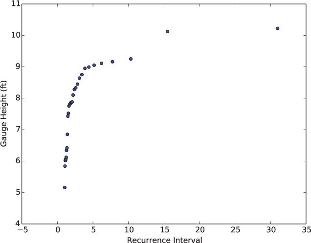
gauge height for each recurrence interval. Once we have this function, we can plug in 100 to find the gauge height for a 100-year flood.
What we need is a regression analysis, as we discussed in Section 8.6. But linear regression only works properly if the data exhibits a linear relationship, i.e., we can draw a straight line that closely approximates the data points.
Reflection 8.33 Do you think we can use linear regression on the data in Figure 8.7?
This data in Figure 8.7 clearly do not have a linear relationship, so a linear regression will not produce a good approximation. The problem is that the x coordinates (recurrence intervals) are increasing multiplicatively rather than additively; the recurrence interval for the flood with rank r + 1 is (r + 1)/r times the recurrence interval for the flood with rank r. However, we will share a trick that allows us to use linear regression anyway. To illustrate the trick we can use to turn this non-linear curve into a “more linear” one, consider the plot on the left in Figure 8.8, representing points (20, 0), (21, 1), (22, 2), ..., (210, 10). Like the plot in Figure 8.7, the x coordinates are increasing multiplicatively; each x coordinate is twice the one before it. The plot on the right in Figure 8.8 contains the points that result from taking the logarithm base 2 of each x coordinate (log2 x), giving
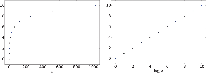
Figure 8.8 On the left is a plot of the points (20, 0), (21, 1), (22, 2), ..., (210, 10), and on the right is a plot of the points that result from taking the logarithm base 2 of the x coordinate of each of these points.
(0, 0), (1, 1), (2, 2), ..., (10, 10). Notice that this has turned an exponential plot into a linear one.
We can apply this same technique to the plotRecurrenceIntervals function you wrote above to make the curve approximately linear. Write a new function
plotLogRecurrenceIntervals(heights)
that modifies the plotRecurrenceIntervals function so that it makes a new list of logarithmic recurrence intervals, and then computes the linear regression line based on these x values. Use logarithms with base 10 for convenience. Then plot the data and the regression line using the linearRegression function from Exercise 8.6.1. To find the 100-year flood gauge height, we want the regression line to extend out to 100 years. Since we are using logarithms with base 10, we want the x coordinates to run from log10 1 = 0 to log10 100 = 2.
Question 8.5.1 Based on Figure 8.8, what is the estimated river level for a 100-year flood? How can you find this value exactly in your program? What is the exact value?
Part 4: An alternative method
As noted earlier in this section, there are seven gauge height values missing from the data file. But all of the peak streamflow values are available. If there is a linear correlation between peak streamflow and gauge height, then it might be more accurate to find the 100-year peak streamflow value instead, and then use the linear regression between peak streamflow and gauge height to find the gauge height that corresponds to the 100-year peak streamflow value.
First, write a function
plotFlowsHeights(flows, heights)
that produces a scatter plot with peak streamflow on the x-axis and the same year’s gauge height on the y axis. Do not plot data for which the gauge height is missing. Then also plot the least squares linear regression for this data.
Next, write a function
plotLogRecurrenceIntervals2(flows)
that modifies the plotLogRecurrenceIntervals function from Part 3 so that it find the 100-year peak streamflow value instead.
Question 8.5.2 What is the 100-year peak streamflow rate?
Once you have found the 100-year peak streamflow rate, use the linear regression formula to find the corresponding 100-year gauge height.
Question 8.5.3 What is the gauge height that corresponds to the 100-year peak streamflow rate?
Question 8.5.4 Compare the two results. Which one do you think is more accurate? Why?
Project 8.6 Voting methods
Although most of us are used to simple plurality-based elections in which the candidate with the most votes wins, there are other voting methods that have been proven to be fairer according to various criteria. In this project, we will investigate two other such voting methods. For all of the parts of the project, we will assume that there are four candidates named Amelia, Beth, Caroline, and David (abbreviated A, B, C, and D).
Part 1: Get the data
The voting results for an election are stored in a data file containing one ballot per line. Each ballot consists of one voter’s ranking of the candidates. For example, a small file might look like:
B A D C
D B A C
B A C D
To begin, write a function
readVotes(fileName)
that returns these voting results as a list containing one list for each ballot. For example, the file above should be stored in a list that looks like this:
[['B', 'A', 'D', 'C'], ['D', 'B', 'A', 'C'], ['A', 'B', 'C', 'D']]
There are three sample voting result files on the book web site. Also feel free to create your own.
Part 2: Plurality voting
First, we will implement basic plurality voting. Write a function
plurality(ballots)
that prints the winner (or winners if there is a tie) of the election based on a plurality count. The parameter of the function is a list of ballots like that returned by the readVotes function. Your function should first iterate over all of the ballots and count the number of first-place votes won by each candidate. Store these votes in a dictionary containing one entry for each candidate. To break the problem into more manageable pieces, write a “helper function”
printWinners(points)
that determines the winner (or winners if there is a tie) based on this dictionary (named points), and then prints the outcome. Call this function from your plurality function.
Part 3: Borda count
Next, we will implement a vote counting system known as a Borda count, named after Jean-Charles de Borda, a mathematician and political scientist who lived in 18th century France. For each ballot in a Borda count, a candidate receives a number of points equal to the number of lower-ranked candidates on the ballot. In other words, with four candidates, the first place candidate on each ballot is awarded three points, the second place candidate is awarded two points, the third place candidate is awarded one point, and the fourth place candidate receives no points. In the example ballot above, candidate B is the winner because candidate A receives 2 + 1 + 2 = 5 points, candidate B receives 3 + 2 + 3 = 8 points, candidate C receives 0 + 0 + 1 = 1 points, and candidate D receives 1 + 3 + 0 = 4 points. Note that, like a plurality count, it is possible to have a tie with a Borda count.
Write a function
borda(ballots)
that prints the winner (or winners if there is a tie) of the election based on a Borda count. Like the plurality function, this function should first iterate over all of the ballots and count the number of points won by each candidate. To make this more manageable, write another “helper function” to call from within your loop named
processBallot(points, ballot)
that processes each individual ballot and adds the appropriate points to the dictionary of accumulated points named points. Once all of the points have been accumulated, call the printWinners above to determine the winner(s) and print the outcome.
Part 4: Condorcet voting
Marie Jean Antoine Nicolas de Caritat, Marquis de Condorcet was another mathematician and political scientist who lived about the same time as Borda. Condorcet proposed a voting method that he considered to be superior to the Borda count. In this method, every candidate participates in a virtual head-to-head election between herself and every other candidate. For each ballot, the candidate who is ranked higher wins. If a candidate wins every one of these head-to-head contests, she is determined to be the Condorcet winner. Although this method favors the candidate who is most highly rated by the majority of voters, it is also possible for there to be no winner.
Write a function
condorcet(ballots)
that prints the Condorcet winner of the election or indicates that there is none. (If there is a winner, there can only be one.)
Suppose that the list of candidates is assigned to candidates. (Think about how you can get this list.) To simulate all head-to-head contests between one candidate named candidate1 and all of the rest, we can use the following for loop:
for candidate2 in candidates:
    if candidate2 != candidate1:
        # head-to-head between candidate1 and candidate2 here
This loop iterates over all of the candidates and sets up a head-to-head contest between each one and candidate1, as long as they are not the same candidate.
Reflection 8.34 How can we now use this loop to generate contests between all pairs of candidates?
To generate all of the contests with all possible values of candidate1, we can nest this for loop in the body of another for loop that also iterates over all of the candidates, but assigns them to candidate1 instead:
for candidate1 in candidates:
    for candidate2 in candidates:
        if candidate2 != candidate1:
            # head-to-head between candidate1 and candidate2 here
Reflection 8.35 This nested for loop actually generates too many pairs of candidates. Can you see why?
To simplify the body of the nested loop (where the comment is currently), write another “helper function”
head2head(ballots, candidate1, candidate2)
that returns the candidate that wins in a head-to-head vote between candidate1 and candidate2, or None is there is a tie. Your condorcet function should call this function for every pair of different candidates. For each candidate, keep track of the number of head-to-head wins in a dictionary with one entry per candidate.
Reflection 8.36 The most straightforward algorithm to decide whether candidate1 beats candidate2 on a particular ballot iterates over all of the candidates on the ballot. Can you think of a way to reorganize the ballot data before calling head2head so that the head2head function can decide who wins each ballot in only one step instead?
Part 5: Compare the three methods
Execute your three functions on each of the three data files on the book web site and compare the results.
Project 8.7 Heuristics for traveling salespeople
Imagine that you drive a delivery truck for one of the major package delivery companies. Each day, you are presented with a list of addresses to which packages must be delivered. Before you can call it a day, you must drive from the distribution center to each package address, and back to the distribution center. This cycle is known as a tour. Naturally, you wish to minimize the total distance that you need to drive to deliver all the packages, i.e., the total length of the tour. For example, Figures 8.9 and 8.10 show two different tours.


This is known as the traveling salesperson problem (TSP), and it is notoriously difficult. In fact, as far as anyone knows, the only way to come up with a guaranteed correct solution is to essentially enumerate all possible tours and choose the best one. But since, for n locations, there are n! (n factorial) different tours, this is practically impossible.
Unfortunately, the TSP has many important applications, several of which seem at first glance to have nothing at all to do with traveling or salespeople, including circuit board drilling, controlling robots, designing networks, x-ray crystallography, scheduling computer time, and assembling genomes. In these cases, a heuristic must be used. A heuristic does not necessarily give the best answer, but it tends to work well in practice
For this project, you will design your own heuristic, and then work with a genetic algorithm, a type of heuristic that mimics the process of evolution to iteratively improve problem solutions.
Part 1: Write some utility functions
Each point on your itinerary will be represented by (x, y) coordinates, and the input to the problem is a list of these points. A tour will also be represented by a list of points; the order of the points indicates the order in which they are visited. We will store a list of points as a list of tuples.
The following function reads in points from a file and returns the points as a list of tuples. We assume that the file contains one point per line, with the x and y coordinates separated by a space.
def readPoints(filename):
    inputFile = open(filename, 'r')
    points = []
    for line in inputFile:
        values = line.split()
        points.append((float(values[0]), float(values[1])))
    return points
To begin, write the following three functions. The first two will be needed by your heuristics, and the third will allow you to visualize the tours that you create. To test your functions, and the heuristics that you will develop below, use the example file containing the coordinates of 96 African cities (africa.tsp) on the book web site.
distance(p, q)returns the distance between pointspandq, each of which is stored as a two-element tuple.tourLength(tour)returns the total length of a tour, stored as a list of tuples. Remember to include the distance from the last point back to the first point.drawTour(tour)draws a tour using turtle graphics. Use thesetworldcoordinatesmethod to make the coordinates in your drawing window more closely match the coordinates in the data files you use. For example, for theafrica.tspdata file, the following will work well:screen.setworldcoordinates(-40, -25, 40, 60)
Part 2: Design a heuristic
Now design your own heuristic to find a good TSP tour. There are many possible ways to go about this. Be creative. Think about what points should be next to each other. What kinds of situations should be fixed? Use the drawTour function to visualize your tours and help you design your heuristic.
Part 3: A genetic algorithm
A genetic algorithm attempts to solve a hard problem by emulating the process of evolution. The basic idea is to start with a population of feasible solutions to the problem, called individuals, and then iteratively try to improve the fitness of this population through the evolutionary operations of recombination and mutation. In genetics, recombination is when chromosomes in a pair exchange portions of their DNA during meiosis. The illustration below shows how a crossover would affect the bases in a particular pair of (single stranded) DNA molecules.
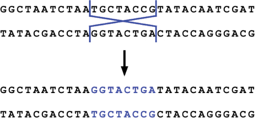
Mutation occurs when a base in a DNA molecule is replaced with a different base or when bases are inserted into or deleted from a sequence. Most mutation is the result of DNA replication errors but environmental factors can also lead to mutations in DNA.
To apply this technique to the traveling salesperson problem, we first need to define what we mean by an individual in a population. In genetics, an individual is represented by its DNA, and an individual’s fitness, for the purposes of evolution, is some measure of how well it will thrive in its environment. In the TSP, we will have a population of tours, so an individual is one particular tour — a list of cities. The most natural fitness function for an individual is the length of the tour; a shorter tour is more fit than a longer tour.
Recombination and mutation on tours are a bit trickier conceptually than they are for DNA. Unlike with DNA, swapping two subsequences of cities between two tours is not likely to produce two new valid tours. For example, suppose we have two tours [a, b, c, d] and [b, a, d, c], where each letter represents a point. Swapping the two middle items between the tours will produce the offspring [a, a, d, d] and [b, b, c, c], neither of which are permutations of the cities. One way around this is to delete from the first tour the cities in the portion to be swapped from the second tour, and then insert this portion from the second tour. In the above example, we would delete points a and d from the first tour, leaving [b, c], before inserting [a, d] in the middle. Doing likewise for the second tour gives us children [b, a, d, c] and [a, b, c, d]. But we are not limited in genetic programming to recombination that more or less mimics that found in nature. A recombination operation can be anything that creates new offspring by somehow combining two parents. A large part of this project involves brainstorming about and experimenting with different techniques.
We must also rethink mutation since we cannot simply replace an arbitrary city with another city and end up with a valid tour. One idea might be to swap the positions of two randomly selected cities instead. But there are other possibilities as well.
Your mission is to improve upon a baseline genetic algorithm for TSP. Be creative! You may change anything you wish as long as the result can still be considered a genetic algorithm. To get started, download the baseline program from the book web site. Try running it with the 96-point instance on the book web site. Take some time to understand how the program works. Ask questions. You may want to refer to the Python documentation if you don’t recall how a particular function works. Most of the work is performed by the following four functions:
makePopulation(cities): creates an initial population (of random tours)crossover(mom, pop): performs a recombination operation on two tours and returns the two offspringmutate(individual): mutates an individual tournewGeneration(population): update the population by performing a crossover and mutating the offspring
Write the function
histogram(population)
that is called from the report function. (Use a Python dictionary.) This function should print a frequency chart (based on tour length) that gives you a snapshot of the diversity in your population. Your histogram function should print something like this:
Population diversity
   1993.2714596455853   :   ****
   2013.1798076309087   :   **
   2015.1395212505120   :   ****
   2017.1005248468230   :   ********************************
   2020.6881282400334   :   *
   2022.9044855489917   :   *
   2030.9623523675089   :   *
   2031.4773010231959   :   *
   2038.0257926528227   :   *
   2040.7438913120230   :   *
   2042.8148398732630   :   *
   2050.1916058477627   :   *
This will be very helpful as you strive to improve the algorithm: recombination in a homogeneous population is not likely to get you very far.
Brainstorm ways to improve the algorithm. Try lots of different things, ranging from tweaking parameters to completely rewriting any of the four functions described above. You are free to change anything, as long as the result still resembles a genetic algorithm. Keep careful records of what works and what doesn’t to include in your submission.
On the book web site is a link to a very good reference [42] that will help you think of new things to try. Take some time to skim the introductory sections, as they will give you a broader sense of the work that has been done on this problem. Sections 2 and 3 contain information on genetic algorithms; Section 5 contains information on various recombination/crossover operations; and Section 7 contains information on possible mutation operations. As you will see, this problem has been well studied by researchers over the past few decades! (To learn more about this history, we recommend In Pursuit of the Traveling Salesman by William Cook [8].)
1SCRABBLE® is a registered trademark of Hasbro Inc.
2These formulas assume that the variances of the x and y errors are equal.
4The data file contains the rows of the file at http://nypd.openscrape.com/#/collisions.csv.gz (accessed October 1, 2013) that involved a bicyclist.
5The data set on the book’s web site is the original file from http://archive.ics.uci.edu/ml/datasets/Breast+Cancer+Wisconsin+(Original) with 16 rows containing missing attributes removed.
6This is a slightly "cleaned" version of the original data file from http://www.es.ucsc.edu/~jzachos/Data/2008CompilationData.xls
7Educational Attainment by Employment Status for the Population 25 to 64 Years (Table B23006), U.S. Census Bureau, 2012 American Community Survey, http://factfinder2.census.gov/faces/tableservices/jsf/pages/productview.xhtml?pid=ACS_12_1YR_B23006
8Adapted from data available at http://onlinestatbook.com/2/case_studies/sat.html
9http://nwis.waterdata.usgs.gov/nwis
10http://nwis.waterdata.usgs.gov/nwis/peak?site_no=13018750&agency_cd=USGS&format=rdb