
CHAPTER 4
Growth and decay
Our population and our use of the finite resources of planet Earth are growing exponentially, along with our technical ability to change the environment for good or ill.
Stephen Hawking
TED talk (2008)
SOME of the most fundamental questions asked in the natural and social sciences concern the dynamic sizes of populations and other quantities over time. For example, we may be interested in the size of a plant population being affected by an invasive species, the magnitude of an infection facing a human population, the quantity of a radioactive material in a storage facility, the penetration of a product in the global marketplace, or the evolving characteristics of a dynamic social network. The possibilities are endless.
To study situations like these, scientists develop a simplified model that abstracts key characteristics of the actual situation so that it might be more easily understood and explored. In this sense, a model is another example of abstraction. Once we have a model that describes the problem, we can write a simulation that shows what happens when the model is applied over time. The power of modeling and simulation lies in their ability to either provide a theoretical framework for past observations or predict future behavior. Scientists often use models in parallel with traditional experiments to compare their observations to a proposed theoretical framework. These parallel scientific processes are illustrated in Figure 4.1. On the left is the computational process. In this case, we use “model” instead of “algorithm” to acknowledge the possibility that the model is mathematical rather than algorithmic. (We will talk more about this process in Section 7.1.) On the right side is the parallel experimental process, guided by the scientific method. The results of the computational and experimental processes can be compared, possibly leading to model adjustments or new experiments to improve the results.

When we model the dynamic behavior of populations, we will assume that time ticks in discrete steps and, at any particular time step, the current population size is based on the population size at the previous time step. Depending on the problem, a time step may be anywhere from a nanosecond to a century. In general, a new time step may bring population increases, in the form of births and immigration, and population decreases, in the form of deaths and emigration. In this chapter, we will discuss a fundamental algorithmic technique, called an accumulator, that we will use to model dynamic processes like these. Accumulators crop up in all kinds of problems, and lie at the foundation of a variety of different algorithmic techniques. We will continue to see examples throughout the book.
4.1 DISCRETE MODELS
Managing a fishing pond
Suppose we manage a fishing pond that contained a population of 12,000 largemouth bass on January 1 of this year. With no fishing, the bass population is expected to grow at a rate of 8% per year, which incorporates both the birth rate and the death rate of the population. The maximum annual fishing harvest allowed is 1,500 bass. Since this is a popular fishing spot, this harvest is attained every year. Is our maximum annual harvest sustainable? If not, how long until the fish population dies out? Should we reduce the maximum harvest? If so, what should it be reduced to?
We can find the projected population size for any given year by starting with the initial population size, and then computing the population size in each successive year based on the size in the previous year. For example, suppose we wanted to know the projected population size four years from now. We start with the initial population of largemouth bass, assigned to a variable named population0:
population0 = 12000
Then we want to set the population size at the end of the first year to be this initial population size, plus 8% of the initial population size, minus 1,500. In other words, if we let population1 represent the population size at the end of the first year, then
population1 = population0 + 0.08 * population0 - 1500 # 11,460
or, equivalently,
population1 = 1.08 * population0 - 1500 # 11,460.0
The population size at the end of the second year is computed in the same way, based on the value of population1:
population2 = 1.08 * population1 - 1500 # 10,876.8
Continuing,
population3 = 1.08 * population2 - 1500    # 10,246.94
population4 = 1.08 * population3 - 1500    # 9,566.6952
So this model projects that the bass population in four years will be 9, 566 (ignoring the “fractional fish” represented by the digits to the right of the decimal point).
The process we just followed was obviously repetitive (or iterative), and is therefore ripe for a for loop. Recall that we used the following for loop in Section 3.2 to draw our geometric flower with eight petals:
for segment in range(8):
    tortoise.forward(length)
    tortoise.left(135)
The keywords for and in are required syntax elements, while the parts in red are up to the programmer. The variable name, in this case segment, is called an index variable. The part in red following in is a list of values assigned to the index variable, one value per iteration. Because range(8) represents a list of integers between 0 and 7, this loop is equivalent to the following sequence of statements:
segment = 0
tortoise.forward(length)
tortoise.left(135)
segment = 1
tortoise.forward(length)
tortoise.left(135)
segment = 2
tortoise.forward(length)
tortoise.left(135)
  ⋮
segment = 7
tortoise.forward(length)
tortoise.left(135)
Because eight different values are assigned to segment, the loop executes the two drawing statements in the body of the loop eight times.
In our fish pond problem, to compute the population size at the end of the fourth year, we performed four computations, namely:
population0 = 12000
population1 = 1.08 * population0 - 1500   # 11460.0
population2 = 1.08 * population1 - 1500   # 10876.8
population3 = 1.08 * population2 - 1500   # 10246.94
population4 = 1.08 * population3 - 1500   # 9566.6952
So we need a for loop that will iterate four times:
for year in range(4):
    # compute population based on previous population
In each iteration of the loop, we want to compute the current year’s population size based on the population size in the previous year. In the first iteration, we want to compute the value that we assigned to population1. And, in the second, third, and fourth iterations, we want to compute the values that we assigned to population2, population3, and population4.
But how do we generalize these four statements into one statement that we can repeat four times? The trick is to notice that, once each variable is used to compute the next year’s population, it is never used again. Therefore, we really have no need for all of these variables. Instead, we can use a single variable population, called an accumulator variable (or just accumulator), that we multiply by 1.08 and subtract 1500 from each year. We initialize population = 12000, and then for each successive year we assign
population = 1.08 * population - 1500
Remember that an assignment statement evaluates the righthand side first. So the value of population on the righthand size of the equals sign is the previous year’s population, which is used to compute the current year’s population that is assigned to population of the lefthand side.
population = 12000
for year in range(4):
    population = 1.08 * population - 1500
This for loop is equivalent to the following statements:

In the first iteration of the for loop, 0 is assigned to year and population is assigned the previous value of population (12000) times 1.08 minus 1500, which is 11460.0. Then, in the second iteration, 1 is assigned to year and population is once again assigned the previous value of population (now 11460.0) times 1.08 minus 1500, which is 10876.8. This continues two more times, until the for loop ends. The final value of population is 9566.6952, as we computed earlier.
Reflection 4.1 Type in the statements above and add the following statement after the assignment to population in the body of the for loop:
print(year + 1, int(population))
Run the program. What is printed? Do you see why?
We see in this example that we can use the index variable year just like any other variable. Since year starts at zero and the first iteration of the loop is computing the population size in year 1, we print year + 1 instead of year.
Reflection 4.2 How would you change this loop to compute the fish population in five years? Ten years?
Changing the number of years to compute is now simple. All we have to do is change the value in the range to whatever we want: range(5), range(10), etc. If we put this computation in a function, then we can have the parameter be the desired number of years:
def pond(years):
    """Simulates a fish population in a fishing pond, and
       prints annual population size.  The population
       grows 8% per year with an annual harvest of 1500.

    Parameter:
        years: number of years to simulate

    Return value: the final population size
    """

    population = 12000
    for year in range(years):
        population = 1.08 * population - 1500
        print(year + 1, int(population))

    return population

def main():
    finalPopulation = pond(10)
    print('The final population is', finalPopulation)

main()
Reflection 4.3 What would happen if population = 12000 was inside the body of the loop instead of before it? What would happen if we omitted the population = 12000 statement altogether?
The initialization of the accumulator variable before the loop is crucial. If population were not initialized before the loop, then an error would occur in the first iteration of the for loop because the righthand side of the assignment statement would not make any sense!
Reflection 4.4 Use the pond function to answer the original questions: Is this maximum harvest sustainable? If not, how long until the fish population dies out? Should the pond manager reduce the maximum harvest? If so, what should it be reduced to?
Calling this function with a large enough number of years shows that the fish population drops below zero (which, of course, can’t really happen) in year 14:
1 11460
2 10876
3 10246
⋮
13 392
14 -1076
⋮
This harvesting plan is clearly not sustainable, so the pond manager should reduce it to a sustainable level. In this case, determining the sustainable level is easy: since the population grows at 8% per year and the pond initially contains 12,000 fish, we cannot allow more than 0.08 · 12000 = 960 fish to be harvested per year without the population declining.
Reflection 4.5 Generalize the pond function with two additional parameters: the initial population size and the annual harvest. Using your modified function, compute the number of fish that will be in the pond in 15 years if we change the annual harvest to 800.
With these modifications, your function might look like this:
def pond(years, initialPopulation, harvest):
    """ (docstring omitted) """

    population = initialPopulation
    for year in range(years):
        population = 1.08 * population - harvest
        print(year + 1, int(population))

    return population
The value of the initialPopulation parameter takes the place of our previous initial population of 12000 and the parameter named harvest takes the place of our previous harvest of 1500. To answer the question above, we can replace the call to the pond function from main with:
finalPopulation = pond(15, 12000, 800)
The result that is printed is:
1 12160
2 12332
3 12519
4 12720
⋮
13 15439
14 15874
15 16344
The final population is 16344.338228396558
Reflection 4.6 How would you call the new version of the pond function to replicate its original behavior, with an annual harvest of 1500?
Before moving on, let’s look at a helpful Python trick, called a format string, that enables us to format our table of annual populations in a more attractive way. To illustrate the use of a format string, consider the following modified version of the previous function.
def pond(years, initialPopulation, harvest):
    """ (docstring omitted) """

    population = initialPopulation
    print('Year | Population')
    print('-----|-----------')
    for year in range(years):
        population = 1.08 * population - harvest
        print('{0:^4} | {1:>9.2f}'.format(year + 1, population))

    return population
The function begins by printing a table header to label the columns. Then, in the call to the print function inside the for loop, we utilize a format string to line up the two values in each row. The syntax of a format string is
'<replacement fields>'.format(<values to format>)
(The parts in red above are descriptive and not part of the syntax.) The period between the the string and format indicates that format is a method of the string class; we will talk more about the string class in Chapter 6. The parameters of the format method are the values to be formatted. The format for each value is specified in a replacement field enclosed in curly braces ({}) in the format string.
In the example in the for loop above, the {0:^4} replacement field specifies that the first (really the “zero-th”; computer scientists like to start counting at 0) argument to format, in this case year + 1, should be centered (^) in a field of width 4. The {1:>9.2f} replacement field specifies that population, as the second argument to format, should be right justified (>) in a field of width 9 as a floating point number with two places to the right of the decimal point (.2f). When formatting floating point numbers (specified by the f), the number before the decimal point in the replacement field is the minimum width, including the decimal point. The number after the decimal point in the replacement field is the minimum number of digits to the right of the decimal point in the number. (If we wanted to align to the left, we would use <.) Characters in the string that are not in replacement fields (in this case, two spaces with a vertical bar between them) are printed as-is. So, if year were assigned the value 11 and population were assigned the value 1752.35171, the above statement would print

To fill spaces with something other than a space, we can use a fill character immediately after the colon. For example, if we replaced the second replacement field with {1:*>9.2f}, the previous statement would print the following instead:

Measuring network value
Now let’s consider a different problem. Suppose we have created a new online social network (or a new group within an existing social network) that we expect to steadily grow over time. Intuitively, as new members are added, the value of the network to its members grows because new relationships and opportunities become available. The potential value of the network to advertisers also grows as new members are added. But how can we quantify this value?
We will assume that, in our social network, two members can become connected or “linked” by mutual agreement, and that connected members gain access to each other’s network profile. The inherent value of the network lies in these connections, or links, rather than in the size of its membership. Therefore, we need to figure out how the potential number of links grows as the number of members grows. The picture below visualizes this growth. The circles, called nodes, represent members of the social network and lines between nodes represent links between members.
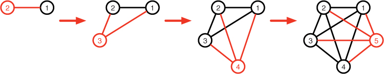
At each step, the red node is added to the network. In each step, the red links represent all of the potential new connections that could result from the addition of the new member.
Reflection 4.7 What is the maximum number of new connections that could arise when each of nodes 2, 3, 4, and 5 are added? In general, what is the maximum number of new connections that could arise from adding node number n?
Node 2 adds a maximum of 1 new connection, node 3 adds a maximum of 2 new connections, node 4 adds a maximum of 3 new connections, etc. In general, a maximum of n – 1 new connections arise from the addition of node number n. This pattern is illustrated in the table below.

Therefore, as shown in the last row, the maximum number of links in a network with n nodes is the sum of the numbers in the second row:
1 + 2 + 3 + . . . + n − 1.
We will use this sum to represent the potential value of the network.
Let’s write a function, similar to the previous one, that lists the maximum number of new links, and the maximum total number of links, as new nodes are added to a network. In this case, we will need an accumulator to count the total number of links. Adapting our pond function to this new purpose gives us the following:
def countLinks(totalNodes):
    """Prints a table with the maximum total number of links
       in networks with 2 through totalNodes nodes.

    Parameter:
        totalNodes: the total number of nodes in the network

    Return value:
        the maximum number of links in a network with totalNodes nodes
    """

    totalLinks = 0
    for node in range(totalNodes):
        newLinks = ???
        totalLinks = totalLinks + newLinks
        print(node, newLinks, totalLinks)

    return totalLinks
In this function, we want our accumulator variable to count the total number of links, so we renamed it from population to to totalLinks, and initialized it to zero. Likewise, we renamed the parameter, which specifies the number of iterations, from years to totalNodes, and we renamed the index variable of the for loop from year to node because it will now be counting the number of the node that we are adding at each step. In the body of the for loop, we add to the accumulator the maximum number of new links added to the network with the current node (we will return to this in a moment) and then print a row containing the node number, the maximum number of new links, and the maximum total number of links in the network at that point.
Before we determine what the value of newLinks should be, we have to resolve one issue. In the table above, the node numbers range from 2 to the number of nodes in the network, but in our for loop, node will range from 0 to totalNodes - 1. This turns out to be easily fixed because the range function can generate a wider variety of number ranges than we have seen thus far. If we give range two arguments instead of one, like range(start, stop), the first argument is interpreted as a starting value and the second argument is interpreted as the stopping value, producing a range of values starting at start and going up to, but not including, stop. For example, range(-5, 10) produces the integers –5,–4,–3, . . ., 8, 9.
To see this for yourself, type range(-5, 10) into the Python shell (or print it in a program).
>>> range(-5, 10)
range(-5, 10)
Unfortunately, you will get a not-so-useful result, but one that we can fix by converting the range to a list of numbers. A list, enclosed in square brackets ([ ]), is another kind of abstract data type that we will make extensive use of in later chapters. To convert the range to a list, we can pass it as an argument to the list function:
>>> list(range(-5, 10))
[-5, -4, -3, -2, -1, 0, 1, 2, 3, 4, 5, 6, 7, 8, 9]
Reflection 4.8 What list of numbers does range(1, 10) produce? What about range(10, 1)? Can you explain why in each case?
Reflection 4.9 Back to our program, what do we want our for loop to look like?
For node to start at 2 and finish at totalNodes, we want our for loop to be
for node in range(2, totalNodes + 1):
Now what should the value of newLinks be in our program? The answer is in the table we constructed above; the maximum number of new links added to the network with node number n is n – 1. In our loop, the node number is assigned to the name node, so we need to add node - 1 links in each step:
newLinks = node - 1
With these substitutions, our function looks like this:
def countLinks(totalNodes):
    """ (docstring omitted) """

    totalLinks = 0
    for node in range(2, totalNodes + 1):
        newLinks = node - 1
        totalLinks = totalLinks + newLinks
        print(node, newLinks, totalLinks)

    return totalLinks

def main():
    links = countLinks(10)
    print('The total number of links is', links)

main()
As with our previous for loop, we can see more clearly what this loop does by looking at an equivalent sequence of statements. The changing value of node is highlighted in red.
totalLinks = 0

node = 2
newLinks = node - 1                 # newLinks is assigned 2 - 1 = 1
totalLinks = totalLinks + newLinks  # totalLinks is assigned 0 + 1 = 1
print(node, newLinks, totalLinks)   # prints 2 1 1

node = 3
newLinks = node - 1                 # newLinks is assigned 3 - 1 = 2
totalLinks = totalLinks + newLinks  # totalLinks is assigned 1 + 2 = 3
print(node, newLinks, totalLinks)   # prints 3 2 3

node = 4
newLinks = node - 1                 # newLinks is assigned 4 - 1 = 3
totalLinks = totalLinks + newLinks  # totalLinks is assigned 3 + 3 = 6
print(node, newLinks, totalLinks)   # prints 4 3 6

 ⋮

node = 10
newLinks = node - 1                 # newLinks is assigned 10 - 1 = 9
totalLinks = totalLinks + newLinks  # totalLinks is assigned 36 + 9 = 45
print(node, newLinks, totalLinks)   # prints 10 9 45
When we call countLinks(10) from the main function above, it prints
2 1 1
3 2 3
4 3 6
5 4 10
6 5 15
7 6 21
8 7 28
9 8 36
10 9 45
The total number of links is 45
We leave lining up the columns more uniformly using a format string as an exercise.
Reflection 4.10 What does countLinks(100) return? What does this represent?
Organizing a concert
Let’s look at one more example. Suppose you are putting on a concert and need to figure out how much to charge per ticket. Your total expenses, for the band and the venue, are $8000. The venue can seat at most 2,000 and you have determined through market research that the number of tickets you are likely to sell is related to a ticket’s selling price by the following relationship:
sales = 2500 - 80 * price
According to this relationship, if you give the tickets away for free, you will overfill your venue. On the other hand, if you charge too much, you won’t sell any tickets at all. You would like to price the tickets somewhere in between, so as to maximize your profit. Your total income from ticket sales will be sales * price, so your profit will be this amount minus $8000.
To determine the most profitable ticket price, we can create a table using a for loop similar to that in the previous two problems. In this case, we would like to iterate over a range of ticket prices and print the profit resulting from each choice. In the following function, the for loop starts with a ticket price of one dollar and adds one to the price in each iteration until it reaches maxPrice dollars.
def profitTable(maxPrice):
    """Prints a table of profits from a show based on ticket price.

    Parameters:
        maxPrice: maximum price to consider

    Return value: None
    """

    print('Price   Income    Profit')
    print('------ --------- ---------')
    for price in range(1, maxPrice + 1):
        sales = 2500 - 80 * price
        income = sales * price
        profit = income - 8000
        formatString = '${0:>5.2f}  ${1:>8.2f}  ${2:8.2f}'
        print(formatString.format(price, income, profit))

def main():
    profitTable(25)

main()
The number of expected sales in each iteration is computed from the value of the index variable price, according to the relationship above. Then we print the price and the resulting income and profit, formatted nicely with a format string. As we did previously, we can look at what happens in each iteration of the loop:
price = 1
sales = 2500 - 80 * price       # sales is assigned 2500 - 80 * 1 = 2420
income = sales * price          # income is assigned  2420 * 1 = 2420
profit = income - 8000          # profit is assigned 2420 - 8000 = -5580
print(price, income, profit)    # prints  $ 1.00   $ 2420.00   $-5580.00

price = 2
sales = 2500 - 80 * price       # sales is assigned 2500 - 80 * 2 = 2340
income = sales * price          # income is assigned  2340 * 2 = 4680
profit = income - 8000          # profit is assigned 4680 - 8000 = -3320
print(price, income, profit)    # prints  $ 2.00   $ 4680.00   $-3320.00

price = 3
sales = 2500 - 80 * price       # sales is assigned 2500 - 80 * 3 = 2260
income = sales * price          # income is assigned  2260 * 3 = 6780
profit = income - 8000          # profit is assigned 6780 - 8000 = -1220
print(price, income, profit)    # prints  $ 3.00   $ 6780.00   $-1220.00
 ⋮
Reflection 4.11 Run this program and determine what the most profitable ticket price is.
The program prints the following table:
Price     Income      Profit
------   ---------   ---------
$ 1.00   $ 2420.00   $-5580.00
$ 2.00   $ 4680.00   $-3320.00
$ 3.00   $ 6780.00   $-1220.00
$ 4.00   $ 8720.00   $  720.00
⋮
$15.00   $19500.00   $11500.00
$16.00   $19520.00   $11520.00
$17.00   $19380.00   $11380.00
⋮
$24.00   $13920.00   $ 5920.00
$25.00   $12500.00   $ 4500.00
The profit in the third column increases until it reaches $11,520.00 at a ticket price of $16, then it drops off. So the most profitable ticket price seems to be $16.
Reflection 4.12 Our program only considered whole dollar ticket prices. How can we modify it to increment the ticket price by fifty cents in each iteration instead?
The range function can only create ranges of integers, so we cannot ask the range function to increment by 0.5 instead of 1. But we can achieve our goal by doubling the range of numbers that we iterate over, and then set the price in each iteration to be the value of the index variable divided by two.
def profitTable(maxPrice):
    """ (docstring omitted) """

    print('Price   Income    Profit')
    print('------ --------- ---------')
    for price in range(1, 2 * maxPrice + 1):
        realPrice = price / 2
        sales = 2500 - 80 * realPrice
        income = sales * realPrice
        profit = income - 8000
        formatString = '${0:>5.2f}  ${1:>8.2f}  ${2:8.2f}'
        print(formatString.format(realPrice, income, profit))
Now when price is 1, the “real price” that is used to compute profit is 0.5. When price is 2, the “real price” is 1.0, etc.
Reflection 4.13 Does our new function find a more profitable ticket price than $16?
Our new function prints the following table.
Price    Income     Profit
------  ---------  ---------
$ 0.50  $ 1230.00  $-6770.00
$ 1.00  $ 2420.00  $-5580.00
$ 1.50  $ 3570.00  $-4430.00
$ 2.00  $ 4680.00  $-3320.00
⋮
$15.50  $19530.00  $11530.00
$16.00  $19520.00  $11520.00
$16.50  $19470.00  $11470.00
⋮
$24.50  $13230.00  $ 5230.00
$25.00  $12500.00  $ 4500.00
If we look at the ticket prices around $16, we see that $15.50 will actually make $10 more.
Just from looking at the table, the relationship between the ticket price and the profit is not as clear as it would be if we plotted the data instead. For example, does profit rise in a straight line to the maximum and then fall in a straight line? Or is it a more gradual curve? We can answer these questions by drawing a plot with turtle graphics, using the goto method to move the turtle from one point to the next.
import turtle

def profitPlot(tortoise, maxPrice):
    """ (docstring omitted) """

    for price in range(1, 2 * maxPrice + 1):
        realPrice = price / 2
        sales = 2500 - 80 * realPrice
        income = sales * realPrice
        profit = income - 8000
        tortoise.goto(realPrice, profit)

def main():
    george = turtle.Turtle()
    screen = george.getscreen()
    screen.setworldcoordinates(0, -15000, 25, 15000)
    profitPlot(george, 25)
    screen.exitonclick()

main()
Our new main function sets up a turtle and then uses the setworldcoordinates function to change the coordinate system in the drawing window to fit the points that we are likely to plot. The first two arguments to setworldcoordinates set the coordinates of the lower left corner of the window, in this case (0,–15, 000). So the minimum visible x value (price) in the window will be zero and the minimum visible y value (profit) will be –15, 000. The second two arguments set the coordinates in the upper right corner of the window, in this case (25, 15,000). So the maximum visible x value (price) will be 25 and the maximum visible y value (profit) will be 15, 000. In the for loop in the profitPlot function, since the first value of realPrice is 0.5, the first goto is
george.goto(0.5, -6770)
which draws a line from the origin (0, 0) to (0.5,–6770). In the next iteration, the value of realPrice is 1.0, so the loop next executes
george.goto(1.0, -5580)
which draws a line from the previous position of (0.5,–6770) to (1.0,–5580). The next value of realPrice is 1.5, so the loop then executes
george.goto(1.5, -4430)
which draws a line from from (1.0,–5580) to (1.5,–4430). And so on, until realPrice takes on its final value of 25 and we draw a line from the previous position of (24.5, 5230) to (25, 4500).
Reflection 4.14 What shape is the plot? Can you see why?
Reflection 4.15 When you run this plotting program, you will notice an ugly line from the origin to the first point of the plot. How can you fix this? (We will leave the answer as an exercise.)
Exercises
Write a function for each of the following problems. When appropriate, make sure the function returns the specified value (rather than just printing it). Be sure to appropriately document your functions with docstrings and comments.
4.1.1. Write a function
print100()
that uses a for loop to print the integers from 0 to 100.
4.1.2. Write a function
triangle1()
that uses a for loop to print the following:
*
**
***
****
*****
******
*******
********
*********
**********
4.1.3. Write a function
square(letter, width)
that prints a square with the given width using the string letter. For example, square('Q', 5) should print:
QQQQQ
QQQQQ
QQQQQ
QQQQQ
QQQQQ
4.1.4. Write a for loop that prints the integers from –50 to 50.
4.1.5. Write a for loop that prints the odd integers from 1 to 100. (Hint: use range(50).)
4.1.6. On Page 43, we talked about how to simulate the minutes ticking on a digital clock using modular arithmetic. Write a function
clock(ticks)
that prints ticks times starting from midnight, where the clock ticks once each minute. To simplify matters, the midnight hour can be denoted 0 instead of 12. For example, clock(100) should print
0:00
0:01
0:02
⋮
0:59
1:00
1:01
⋮
1:38
1:39
To line up the colons in the times and force the leading zero in the minutes, use a format string like this:
print('{0:>2}:{1:0>2}'.format(hours, minutes))
4.1.7. There are actually three forms of the range function:
1 parameter:
range(stop)2 parameters:
range(start, stop)3 parameters:
range(start, stop, skip)
With three arguments, range produces a range of integers starting at the start value and ending at or before stop - 1, adding skip each time. For example,
range(5, 15, 2)
produces the range of numbers 5, 7, 9, 11, 13 and
range(-5, -15, -2)
produces the range of numbers -5, -7, -9, -11, -13. To print these numbers, one per line, we can use a for loop:
for number in range(-5, -15, -2):
    print(number)
- Write a
forloop that prints the even integers from 2 to 100, using the third form of therangefunction. - Write a
forloop that prints the odd integers from 1 to 100, using the third form of therangefunction. - Write a
forloop that prints the integers from 1 to 100 in descending order. - Write a
forloop that prints the values 7, 11, 15, 19. - Write a
forloop that prints the values 2, 1, 0, –1, –2. - Write a
forloop that prints the values –7, –11, –15, –19.
4.1.8. Write a function
multiples(n)
that prints all of the multiples of the parameter n between 0 and 100, inclusive. For example, if n were 4, the function should print the values 0, 4, 8, 12, . . . .
4.1.9. Write a function
countdown(n)
that prints the integers between 0 and n in descending order. For example, if n were 5, the function should print the values 5, 4, 3, 2, 1, 0.
4.1.10. Write a function
triangle2()
that uses a for loop to print the following:
*****
****
***
**
*
4.1.11. Write a function
triangle3()
that uses a for loop to print the following:
******
 *****
  ****
   ***
    **
     *
4.1.12. Write a function
diamond()
that uses for loops to print the following:
***** *****
****   ****
***     ***
**       **
*         *
*         *
**       **
***     ***
****   ****
***** *****
4.1.13. Write a function
circles(tortoise)
that uses turtle graphics and a for loop to draw concentric circles with radii 10, 20, 30, . . ., 100. (To draw each circle, you may use the turtle graphics circle method or the drawCircle function you wrote in Exercise 3.3.8.
4.1.14. In the profitPlot function in the text, fix the problem raised by Reflection 4.15.
plotSine(tortoise, n)
that uses turtle graphics to plot sin x from x = 0 to x = n degrees. Use setworldcoordinates to make the x coordinates of the window range from 0 to 1080 and the y coordinates range from -1 t0 1.
4.1.16. Python also allows us to pass function names as parameters. So we can generalize the function in Exercise 4.1.15 to plot any function we want. We write a function
plot(tortoise, n, f)
where f is the name of an arbitrary function that takes a single numerical argument and returns a number. Inside the for loop in the plot function, we can apply the function f to the index variable x with
tortoise.goto(x, f(x))
To call the plot function, we need to define one or more functions to pass in as arguments. For example, to plot x2, we can define
def square(x):
   return x * x
and then call plot with
plot(george, 20, square)
Or, to plot an elongated sin x, we could define
def sin(x):
   return 10 * math.sin(x)
and then call plot with
plot(george, 20, sin)
After you create your new version of plot, also create at least one new function to pass into plot for the parameter f. Depending on the functions you pass in, you may need to adjust the window coordinate system with setworldcoordinates.
4.1.17. Modify the profitTable function so that it considers all ticket prices that are multiples of a quarter.
4.1.18. Generalize the pond function so that it also takes the annual growth rate as a parameter.
4.1.19. Generalize the pond function further to allow for the pond to be annually restocked with an additional quantity of fish.
4.1.20. Modify the countLinks function so that it prints a table like the following:
|       |   Links     |
| Nodes | New | Total |
| ----- | --- | ----- |
|   2   | 1   |     1 |
|   3   | 2   |     3 |
|   4   | 3   |     6 |
|   5   | 4   |    10 |
|   6   | 5   |    15 |
|   7   | 6   |    21 |
|   8   | 7   |    28 |
|   9   | 8   |    36 |
|  10   | 9   |    45 |
growth1(totalDays)
that simulates a population growing by 3 individuals each day. For each day, print the day number and the total population size.
4.1.22. Write a function
growth2(totalDays)
that simulates a population that grows by 3 individuals each day but also shrinks by, on average, 1 individual every 2 days. For each day, print the day number and the total population size.
growth3(totalDays)
that simulates a population that increases by 110% every day. Assume that the initial population size is 10. For each day, print the day number and the total population size.
4.1.24. Write a function
growth4(totalDays)
that simulates a population that grows by 2 on the first day, 4 on the second day, 8 on the third day, 16 on the fourth day, etc. Assume that the initial population size is 10. For each day, print the day number and the total population size.
sum(n)
that returns the sum of the integers between 1 and n, inclusive. For example, sum(4) returns 1 + 2 + 3 + 4 = 10. (Use a for loop; if you know a shortcut, don’t use it.)
4.1.26. Write a function
sumEven(n)
that returns the sum of the even integers between 2 and n, inclusive. For example, sumEven(6) returns 2 + 4 + 6 = 12. (Use a for loop.)
4.1.27. Between the ages of three and thirteen, girls grow an average of about six centimeters per year. Write a function
growth(finalAge)
that prints a simple height chart based on this information, with one entry for each age, assuming the average girl is 95 centimeters (37 inches) tall at age three.
4.1.28. Write a function
average(low, high)
that returns the average of the integers between low and high, inclusive. For example, average(3, 6) returns (3 + 4 + 5 + 6)/4 = 4.5.
factorial(n)
that returns the value of n! = 1 × 2 × 3 × . . . × (n – 1) × n. (Be careful; how should the accumulator be initialized?)
4.1.30. Write a function
power(base, exponent)
that returns the value of base raised to the exponent power, without using the ** operator. Assume that exponent is a positive integer.
4.1.31. The geometric mean of n numbers is defined to be the nth root of the product of the numbers. (The nth root is the same as the 1/n power.) Write a function
geoMean(high)
that returns the geometric mean of the numbers between 1 and high, inclusive.
4.1.32. Write a function
sumDigits(number, numDigits)
that returns the sum of the individual digits in a parameter number that has numDigits digits. For example, sumDigits(1234, 4) should return the value 1 + 2 + 3 + 4 = 10. (Hint: use a for loop and integer division (// and %).)
4.1.33. Consider the following fun game. Pick any positive integer less than 100 and add the squares of its digits. For example, if you choose 25, the sum of the squares of its digits is 22 + 52 = 29. Now make the answer your new number, and repeat the process. For example, if we continue this process starting with 25, we get: 25, 29, 85, 89, 145, 42, etc.
Write a function
fun(number, iterations)
that prints the sequence of numbers generated by this game, starting with the two digit number, and continuing for the given number of iterations. It will be helpful to know that no number in a sequence will ever have more than three digits. Execute your function with every integer between 15 and 25, with iterations at least 30. What do you notice? Can you classify each of these integers into one of two groups based on the results?
4.1.34. You have $1,000 to invest and need to decide between two savings accounts. The first account pays interest at an annual rate of 1% and is compounded daily, meaning that interest is earned daily at a rate of (1/365)%. The second account pays interest at an annual rate of 1.25% but is compounded monthly. Write a function
interest(originalAmount, rate, periods)
that computes the interest earned in one year on originalAmount dollars in an account that pays the given annual interest rate, compounded over the given number of periods. Assume the interest rate is given as a percentage, not a fraction (i.e., 1.25 vs. 0.0125). Use the function to answer the original question.
4.1.35. Suppose you want to start saving a certain amount each month in an investment account that compounds interest monthly. To determine how much money you expect to have in the future, write a function
invest(investment, rate, years)
that returns the income earned by investing investment dollars every month in an investment account that pays the given rate of return, compounded monthly (rate / 12 % each month).
4.1.36. A mortgage loan is charged some rate of interest every month based on the current balance on the loan. If the annual interest rate of the mortgage is r%, then interest equal to r/12 % of the current balance is added to the amount owed each month. Also each month, the borrower is expected to make a payment, which reduces the amount owed.
Write a function
mortgage(principal, rate, years, payment)
that prints a table of mortgage payments and the remaining balance every month of the loan period. The last payment should include any remaining balance. For example, paying $1,000 per month on a $200,000 loan at 4.5% for 30 years should result in the following table:
Month   Payment     Balance
1       1000.00   199750.00
2       1000.00   199499.06
3       1000.00   199247.18
⋮
359     1000.00    11111.79
360    11153.46        0.00
4.1.37. Suppose a bacteria colony grows at a rate of 10% per hour and that there are initially 100 bacteria in the colony. Write a function
bacteria(days)
that returns the number of bacteria in the colony after the given number of days. How many bacteria are in the colony after one week?
4.1.38. Generalize the function that you wrote for the previous exercise so that it also accepts parameters for the initial population size and the growth rate. How many bacteria are in the same colony after one week if it grows at 15% per hour instead?
4.2 VISUALIZING POPULATION CHANGES
Visualizing changes in population size over time will provide more insight into how population models evolve. We could plot population changes with turtle graphics, as we did in Section 4.1, but instead, we will use a dedicated plotting module called matplotlib, so-named because it emulates the plotting capabilities of the technical programming language MATLAB1. If you do not already have matplotlib installed on your computer, see Appendix A for instructions.
To use matplotlib, we first import the module using
import matplotlib.pyplot as pyplot
matplotlib.pyplot is the name of module; “as pyplot” allows us to refer to the module in our program with the abbreviation pyplot instead of its rather long full name. The basic plotting functions in matplotlib take two arguments: a list of x values and an associated list of y values. A list in Python is an object of the list class, and is represented as a comma-separated sequence of items enclosed in square brackets, such as
[4, 7, 2, 3.1, 12, 2.1]
We saw lists briefly in Section 4.1 when we used the list function to visualize range values; we will use lists much more extensively in Chapter 8. For now, we only need to know how to build a list of population sizes in our for loop so that we can plot them. Let’s look at how to do this in the fishing pond function from Page 119, reproduced below.
def pond(years, initialPopulation, harvest):
    """ (docstring omitted) """

    population = initialPopulation
    print('Year Population')
    for year in range(years):
        population = 1.08 * population - harvest
        print('{0:^4} {1:>9.2f}'.format(year + 1, population))

    return population
We start by creating an empty list of annual population sizes before the loop:
populationList = [ ]
As you can see, an empty list is denoted by two square brackets with nothing in between. To add an annual population size to the end of the list, we will use the append method of the list class. We will first append the initial population size to the end of the empty list with
populationList.append(initialPopulation)
If we pass in 12000 for the initial population parameter, this will result in populationList becoming the single-element list [12000]. Inside the loop, we want to append each value of population to the end of the growing list with
populationList.append(population)
Incorporating this code into our pond function, and deleting the calls to print, yields:
def pond(years, initialPopulation, harvest):
    """Simulates a fish population in a fishing pond, and
       plots annual population size.  The population
       grows 8% per year with an annual harvest.

    Parameters:
       years: number of years to simulate
       initialPopulation: the initial population size
       harvest: the size of the annual harvest

    Return value: the final population size
    """

    population = initialPopulation
    populationList = [ ]
    populationList.append(initialPopulation)
    for year in range(years):
        population = 1.08 * population - harvest
        populationList.append(population)

    return population
The table below shows how the populationList grows with each iteration by appending the current value of population to its end, assuming an initial population of 12,000. When the loop finishes, we have years + 1 population sizes in our list.


There is a strong similarity between the manner in which we are appending elements to a list and the accumulators that we have been talking about in this chapter. In an accumulator, we accumulate values into a sum by repeatedly adding new values to a running sum. The running sum changes (usually grows) in each iteration of the loop. With the list in the for loop above, we are accumulating values in a different way—by repeatedly appending them to the end of a growing list. Therefore, we call this technique a list accumulator.
We now want to use this list of population sizes as the list of y values in a matplotlib plot. For the x values, we need a list of the corresponding years, which can be obtained with range(years + 1). Once we have both lists, we can create a plot by calling the plot function and then display the plot by calling the show function:
pyplot.plot(range(years + 1), populationList)
pyplot.show()
The first argument to the plot function is the list of x values and the second parameter is the list of y values. The matplotlib module includes many optional ways to customize our plots before we call show. Some of the simplest are functions that label the x and y axes:
pyplot.xlabel('Year')
pyplot.ylabel('Fish Population Size')
Incorporating the plotting code yields the following function, whose output is shown in Figure 4.2.
import matplotlib.pyplot as pyplot

def pond(years, initialPopulation, harvest):
    """ (docstring omitted) """

    population = initialPopulation
    populationList = [ ]
    populationList.append(initialPopulation)
    for year in range(years):
        population = 1.08 * population - harvest
        populationList.append(population)

    pyplot.plot(range(years + 1), populationList)
    pyplot.xlabel('Year')
    pyplot.ylabel('Fish Population Size')
    pyplot.show()

    return population
For more complex plots, we can alter the scales of the axes, change the color and style of the curves, and label multiple curves on the same plot. See Appendix B.4 for a sample of what is available. Some of the options must be specified as keyword arguments of the form name = value. For example, to color a curve in a plot red and specify a label for the plot legend, you would call something like this:
pyplot.plot(x, y, color = 'red', label = 'Bass population')
pyplot.legend()    # creates a legend from labeled lines
Exercises
4.2.1. Modify the countLinks function on Page 123 so that it uses matplotlib to plot the number of nodes on the x axis and the maximum number of links on the y axis. Your resulting plot should look like the one in Figure 4.3.
4.2.2. Modify the profitPlot function on Page 128 so that it uses matplotlib to plot ticket price on the x axis and profit on the y axis. (Remove the tortoise parameter.) Your resulting plot should look like the one in Figure 4.4. To get the correct prices (in half dollar increments) on the x axis, you will need to create a second list of x values and append the realPrice to it in each iteration.
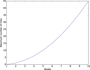
Figure 4.3 Plot for Exercise 4.2.1.

Figure 4.4 Plot for Exercise 4.2.2.
4.2.3. Modify your growth1 function from Exercise 4.1.21 so that it uses matplotlib to plot days on the x axis and the total population on the y axis. Create a plot that shows the growth of the population over 30 days.
4.2.4. Modify your growth3 function from Exercise 4.1.23 so that it uses matplotlib to plot days on the x axis and the total population on the y axis. Create a plot that shows the growth of the population over 30 days.
4.2.5. Modify your invest function from Exercise 4.1.35 so that it uses matplotlib to plot months on the x axis and your total accumulated investment amount on the y axis. Create a plot that shows the growth of an investment of $50 per month for ten years growing at an annual rate of 8%.
4.3 CONDITIONAL ITERATION
In our fishing pond model, to determine when the population size fell below zero, it was sufficient to simply print the annual population sizes for at least 14 years, and look at the results. However, if it had taken a thousand years for the population size to fall below zero, then looking at the output would be far less convenient. Instead, we would like to have a program tell us the year directly, by ceasing to iterate when population drops to zero, and then returning the year it happened. This is a different kind of problem because we no longer know how many iterations are required before the loop starts. In other words, we have no way of knowing what value to pass into range in a for loop.
Instead, we need a more general kind of loop that will iterate only while some condition is met. Such a loop is generally called a while loop. In Python, a while loop looks like this:
while <condition>:
    <body>
The <condition> is replaced with a Boolean expression that evaluates to True or False, and the <body> is replaced with statements constituting the body of the loop. The loop checks the value of the condition before each iteration. If the condition is true, it executes the statements in the body of the loop, and then checks the condition again. If the condition is false, the body of the loop is skipped, and the loop ends.
We will talk more about building Boolean expressions in the next chapter; for now we will only need very simple ones like population > 0. This Boolean expression is true if the value of population is positive, and false otherwise. Using this Boolean expression in the while loop in the following function, we can find the year that the fish population drops to 0.
def yearsUntilZero(initialPopulation, harvest):
    """Computes # of years until a fish population reaches zero.
       Population grows 8% per year with an annual harvest.

    Parameters:
        initialPopulation: the initial population size
        harvest: the size of the annual harvest

    Return value: year during which the population reaches zero
    """

    population = initialPopulation
    year = 0
    while population > 0:
        population = 1.08 * population - harvest
        year = year + 1
    return year
Let’s assume that initialPopulation is 12000 and harvest is 1500, as in our original pond function in Section 4.1. Therefore, before the loop, population is 12000 and year is 0. Since population > 0 is true, the loop body executes, causing population to become 11460 and year to become 1. (You might want to refer back to the annual population sizes on Page 118.) We then go back to the top of the loop to check the condition again. Since population > 0 is still true, the loop body executes again, causing population to become 10876 and year to become 2. Iteration continues until year reaches 14. In this year, population becomes -1076.06. When the condition is checked now, we find that population > 0 is false, so the loop ends and the function returns 14.
Using while loops can be tricky for two reasons. First, a while loop may not iterate at all. For example, if the initial value of population were zero, the condition in the while loop will be false before the first iteration, and the loop will be over before it starts.
Reflection 4.16 What will be returned by the function in this case?
A loop that sometimes does not iterate at all is generally not a bad thing, and can even be used to our advantage. In this case, if population were initially zero, the function would return zero because the value of year would never be incremented in the loop. And this is correct; the population dropped to zero in year zero, before the clock started ticking beyond the initial population size. But it is something that one should always keep in mind when designing algorithms involving while loops.
Second, a while loop may become an infinite loop. For example, suppose initialPopulation is 12000 and harvest is 800 instead of 1500. In this case, as we saw on Page 119, the population size increases every year instead. So the population size will never reach zero and the loop condition will never be false, so the loop will iterate forever. For this reason, we must always make sure that the body of a while loop makes progress toward the loop condition becoming false.
Let’s look at one more example. Suppose we have $1000 to invest and we would like to know how long it will take for our money to double in size, growing at 5% per year. To answer this question, we can create a loop like the following that compounds 5% interest each year:
amount = 1000
while ???:
    amount = 1.05 * amount
print(amount)
Reflection 4.17 What should be the condition in the while loop?
We want the loop to stop iterating when amount reaches 2000. Therefore, we want the loop to continue to iterate while amount < 2000.
amount = 1000
while amount < 2000:
    amount = 1.05 * amount
print(amount)
Reflection 4.18 What is printed by this block of code? What does this result tell us?
Once the loop is done iterating, the final amount is printed (approximately $2078.93), but this does not answer our question.
Reflection 4.19 How do figure out how many years it takes for the $1000 to double?
To answer our question, we need to count the number of times the while loop iterates, which is very similar to what we did in the yearsUntilZero function. We can introduce another variable that is incremented in each iteration, and print its value after the loop, along with the final value of amount:
amount = 1000
while amount < 2000:
    amount = 1.05 * amount
    year = year + 1
print(year, amount)
Reflection 4.20 Make these changes and run the code again. Now what is printed?
Oops, an error message is printed, telling us that the name year is undefined.
Reflection 4.21 How do we fix the error?
The problem is that we did not initialize the value of year before the loop. Therefore, the first time year = year + 1 was executed, year was undefined on the right side of the assignment statement. Adding one statement before the loop fixes the problem:
amount = 1000
year = 0
while amount < 2000:
    amount = 1.05 * amount
    year = year + 1
print(year, amount)
Reflection 4.22 Now what is printed by this block of code? In other words, how many years until the $1000 doubles?
We will see some more examples of while loops later in this chapter, and again in Section 5.5.
Exercises
4.3.1. Suppose you put $1000 into the bank and you get a 3% interest rate compounded annually. How would you use a while loop to determine how long will it take for your account to have at least $1200 in it?
4.3.2. Repeat the last question, but this time write a function
interest(amount, rate, target)
that takes the initial amount, the interest rate, and the target amount as parameters. The function should return the number of years it takes to reach the target amount.
4.3.3. Since while loops are more general than for loops, we can emulate the behavior of a for loop with a while loop. For example, we can emulate the behavior of the for loop
for counter in range(10):
    print(counter)
with the while loop
counter = 0
while counter < 10:
    print(counter)
    counter = counter + 1
Execute both loops “by hand” to make sure you understand how these loops are equivalent.
- What happens if we omit
counter = 0before thewhileloop? Why does this happen? - What happens if we omit
counter = counter + 1from the body of thewhileloop? What does the loop print? - Show how to emulate the following
forloop with awhileloop:for index in range(3, 12):
print(index) - Show how to emulate the following
forloop with awhileloop:for index in range(12, 3, -1):
print(index)
4.3.4. In the profitTable function on Page 127, we used a for loop to indirectly consider all ticket prices divisible by a half dollar. Rewrite this function so that it instead uses a while loop that increments price by $0.50 in each iteration.
4.3.5. A zombie can convert two people into zombies everyday. Starting with just one zombie, how long would it take for the entire world population (7 billion people) to become zombies? Write a function
zombieApocalypse()
that returns the answer to this question.
4.3.6. Tribbles increase at the rate of 50% per hour (rounding down if there are an odd number of them). How long would it take 10 tribbles to reach a population size of 1 million? Write a function
tribbleApocalypse()
that returns the answer to this question.
4.3.7. Vampires can each convert v people a day into vampires. However, there is a band of vampire hunters that can kill k vampires per day. If a coven of vampires starts with vampires members, how long before a town with a population of people becomes a town with no humans left in it? Write a function
vampireApocalypse(v, k, vampires, people)
that returns the answer to this question.
4.3.8. An amoeba can split itself into two once every h hours. How many hours does it take for a single amoeba to become target amoebae? Write a function
amoebaGrowth(h, target)
that returns the answer to this question.
*4.4 CONTINUOUS MODELS
If we want to more accurately model the situation in our fishing pond, we need to acknowledge that the size of the fish population does not really change only once a year. Like virtually all natural processes, the change happens continually or, mathematically speaking, continuously, over time. To more accurately model continuous natural processes, we need to update our population size more often, using smaller time steps. For example, we could update the size of the fish population every month instead of every year by replacing every annual update of
population = population + 0.08 * population - 1500
with twelve monthly updates:
for month in range(12):
    population = population + (0.08 / 12) * population - (1500 / 12)
Since both the growth rate of 0.08 and the harvest of 1500 are based on 1 year, we have divided both of them by 12.
Reflection 4.23 Is the final value of population the same in both cases?
If the initial value of population is 12000, the value of population after one annual update is 11460.0 while the final value after 12 monthly updates is 11439.753329049303. Because the rate is “compounding” monthly, it reduces the population more quickly.
This is exactly how bank loans work. The bank will quote an annual percentage rate (APR) of, say, 6% (or 0.06) but then compound interest monthly at a rate of 6/12% = 0.5% (or 0.005), which means that the actual annual rate of interest you are being charged, called the annual percentage yield (APY), is actually (1+0.005)12−1 ≈ 0.0617 = 6.17%. The APR, which is really defined to be the monthly rate times 12, is sometimes also called the “nominal rate.” So we can say that our fish population is increasing at a nominal rate of 8%, but updated every month.
Difference equations
A population model like this is expressed more accurately with a difference equation, also known as a recurrence relation. If we let P(t) represent the size of the fish population at the end of year t, then the difference equation that defines our original model is

or, equivalently,
P(t) = 1.08 · P(t – 1) – 1500.
In other words, the size of the population at the end of year t is 1.08 times the size of the population at the end of the previous year (t – 1), minus 1500. The initial population or, more formally, the initial condition is P(0) = 12, 000. We can find the projected population size for any given year by starting with P(0), and using the difference equation to compute successive values of P(t). For example, suppose we wanted to know the projected population size four years from now, represented by P(4). We start with the initial condition: P(0) = 12, 000. Then, we apply the difference equation to t = 1:
P(1) = 1.08 · P(0) – 1500 = 1.08 · 12, 000 – 1500 = 11, 460.
Now that we have P(1), we can compute P(2):
P(2) = 1.08 · P(1) – 1500 = 1.08 · 11, 460 – 1500 = 10, 876.8.
Continuing,
P(3) = 1.08 · P(2) – 1500 = 1.08 · 10, 876.8 – 1500 = 10, 246.94
and
P(4) = 1.08 · P(3) – 1500 = 1.08 · 10, 246.94 – 1500 = 9, 566.6952.
So this model projects that the bass population in 4 years will be 9, 566. This is the same process we followed in our for loop in Section 4.1.
To turn this discrete model into a continuous model, we define a small update interval, which is customarily named Δt (Δ represents “change,” so Δt represents “change in time”). If, for example, we want to update the size of our population every month, then we let Δt = 1/12. Then we express our difference equation as
P(t) = P(t – Δt) + (0.08 ·P(t – Δt) – 1500) · Δt
This difference equation is defining the population size at the end of year t in terms of the population size one Δt fraction of a year ago. For example, if t is 3 and Δt is 1/12, then P(t) represents the size of the population at the end of year 3 and P(t – Δt) represents the size of the population at the end of “year 21112for loop on Page 145.
To implement this model, we need to make some analogous changes to the algorithm from Page 119. First, we need to pass in the value of Δt as a parameter so that we have control over the accuracy of the approximation. Second, we need to modify the number of iterations in our loop to reflect 1/Δt decay events each year; the number of iterations becomes years · (1/Δt) = years/Δt. Third, we need to alter how the accumulator is updated in the loop to reflect this new type of difference equation. These changes are reflected below. We use dt to represent Δt.

def pond(years, initialPopulation, harvest, dt):
    """ (docstring omitted) """

    population = initialPopulation
    for step in range(1, int(years / dt) + 1):
        population = population + (0.08 * population - harvest) * dt

    return population
Reflection 4.24 Why do we use range(1, int(years / dt) + 1) in the for loop instead of range(int(years / dt))?
We start the for loop at one instead of zero because the first iteration of the loop represents the first time step of the simulation. The initial population size assigned to population before the loop represents the population at time zero.
To plot the results of this simulation, we use the same technique that we used in Section 4.2. But we also use a list accumulator to create a list of time values for the x axis because the values of the index variable step no longer represent years. In the following function, the value of step * dt is assigned to the variable t, and then appended to a list named timeList.
import matplotlib.pyplot as pyplot

def pond(years, initialPopulation, harvest, dt):
    """Simulates a fish population in a fishing pond, and plots
       annual population size.  The population grows at a nominal
       annual rate of 8% with an annual harvest.

    Parameters:
        years: number of years to simulate
        initialPopulation: the initial population size
        harvest: the size of the annual harvest
        dt: value of "Delta t" in the simulation (fraction of a year)

    Return value: the final population size
    """


    population = initialPopulation
    populationList = [initialPopulation]
    timeList = [0]
    t = 0
    for step in range(1, int(years / dt) + 1):
        population = population + (0.08 * population - harvest) * dt
        populationList.append(population)
        t = step * dt
        timeList.append(t)

    pyplot.plot(timeList, populationList)
    pyplot.xlabel('Year')
    pyplot.ylabel('Fish Population Size')
    pyplot.show()
    return population
Figure 4.5 shows a plot produced by calling this function with Δt = 0.01. Compare this plot to Figure 4.2. To actually come close to approximating a real continuous process, we need to use very small values of Δt. But there are tradeoffs involved in doing so, which we discuss in more detail later in this section.
Radiocarbon dating
When archaeologists wish to know the ages of organic relics, they often turn to radiocarbon dating. Both carbon-12 (12C) and carbon-14 (or radiocarbon, 14C) are isotopes of carbon that are present in our atmosphere in a relatively constant proportion. While carbon-12 is a stable isotope, carbon-14 is unstable and decays at a known rate. All living things ingest both isotopes, and die possessing them in the same proportion as the atmosphere. Thereafter, an organism’s acquired carbon-14 decays at a known rate, while its carbon-12 remains intact. By examining the current ratio of carbon-12 to carbon-14 in organic remains (up to about 60,000 years old), and comparing this ratio to the known ratio in the atmosphere, we can approximate how long ago the organism died.
The annual decay rate (more correctly, the decay constant2) of carbon-14 is about
k = –0.000121.
Radioactive decay is a continuous process, rather than one that occurs at discrete intervals. Therefore, Q(t), the quantity of carbon-14 present at the beginning of year t, needs to be defined in terms of the value of Q(t – Δt), the quantity of carbon-14 a small Δt fraction of a year ago. Therefore, the difference equation modeling the decay of carbon-14 is
Q(t) = Q(t – Δt) + k · Q(t – Δt) · Δt.
Since the decay constant k is based on one year, we scale it down for an interval of length Δt by multiplying it by Δt. We will represent the initial condition with Q(0) = q, where q represents the initial quantity of carbon-14.
Although this is a completely different application, we can implement the model the same way we implemented our continuous fish population model.
import matplotlib.pyplot as pyplot

def decayC14(originalAmount, years, dt):
    """Approximates the continuous decay of carbon-14.

    Parameters:
        originalAmount: the original quantity of carbon-14 (g)
        years: number of years to simulate
        dt: value of "Delta t" in the simulation (fraction of a year)

    Return value: final quantity of carbon-14 (g)
    """

    k = -0.000121
    amount = originalAmount
    t = 0
    timeList = [0]                    # x values for plot
    amountList = [amount]             # y values for plot

    for step in range(1, int(years/dt) + 1):
        amount = amount + k * amount * dt
        t = step * dt
        timeList.append(t)
        amountList.append(amount)

    pyplot.plot(timeList, amountList)
    pyplot.xlabel('Years')
    pyplot.ylabel('Quantity of carbon-14')
    pyplot.show()

    return amount

Like all of our previous accumulators, this function initializes our accumulator variable, named amount, before the loop. Then the accumulator is updated in the body of the loop according to the difference equation above. Figure 4.6 shows an example plot from this function.
Reflection 4.25 How much of 100 g of carbon-14 remains after 5,000 years of decay? Try various Δt values ranging from 1 down to 0.001. What do you notice?
Tradeoffs between accuracy and time
Approximations of continuous models are more accurate when the value of Δt is smaller. However, accuracy has a cost. The decayC14 function has time complexity proportional to y/Δt, where y is the number of years we are simulating, since this is how many times the for loop iterates. So, if we want to improve accuracy by dividing Δt in half, this will directly result in our algorithm requiring twice as much time to run. If we want Δt to be one-tenth of its current value, our algorithm will require ten times as long to run.
Box 4.1: Differential equations
If you have taken a course in calculus, you may recognize each of these continuous models as an approximation of a differential equation. A differential equation is an equation that relates a function to the rate of change of that function, called the derivative. For example, the differential equation corresponding to the carbon-14 decay problem is
dQdt=kQ
where Q is the quantity of carbon-14, dQ/dt is the rate of change in the quantity of carbon-14 at time t (i.e., the derivative of Q with respect to t), and k is the decay constant. Solving this differential equation using basic calculus techniques yields
Q(t) = Q(0) ekt
where Q(0) is the original amount of carbon-14. We can use this equation to directly compute how much of 1000 g of carbon-14 would be left after 2,000 years with:
Q(2000) = 1000 e2000k ≈ 785.0562.
Although simple differential equations like this are easily solved if you know calculus, most realistic differential equations encountered in the sciences are not, making approximate iterative solutions essential. The approximation technique we are using in this chapter, called Euler’s method, is the most fundamental, and introduces error proportional to Δt. More advanced techniques seek to reduce the approximation error further.
To get a sense of how decreasing values of Δt affect the outcome, let’s look at what happens in our decayC14 function with originalAmount = 1000 and years = 2000. The table below contains these results, with the theoretically derived answer in the last row (see Box 4.1). The error column shows the difference between the result and this value for each value of dt. All values are rounded to three significant digits to reflect the approximate nature of the decay constant. We can see from the table that smaller values of dt do indeed provide closer approximations.

Reflection 4.26 What is the relationship between the value of dt and the error? What about between the value of dt and the execution time?
Each row in the table represents a computation that took ten times as long as that in the previous row because the value of dt was ten times smaller. But the error is also ten times smaller. Is this tradeoff worthwhile? The answer depends on the situation. Certainly using dt = 0.0001 is not worthwhile because it gives the same answer (to three significant digits) as dt = 0.001, but takes ten times as long.
These types of tradeoffs — quality versus cost — are common in all fields, and computer science is no exception. Building a faster memory requires more expensive technology. Ensuring more accurate data transmission over networks requires more overhead. And finding better approximate solutions to hard problems requires more time.
Propagation of errors
In both the pond and decayC14 functions in this section, we skirted a very subtle error that is endemic to numerical computer algorithms. Recall from Section 2.2 that computers store numbers in binary and with finite precision, resulting in slight errors, especially with very small floating point numbers. But a slight error can become magnified in an iterative computation. This would have been the case in the for loops in the pond and decayC14 functions if we had accumulated the value of t by adding dt in each iteration with
t = t + dt
instead of getting t by multiplying dt by step. If dt is very small, then there might have been a slight error every time dt was added to t. If the loop iterates for a long time, the value of t will become increasingly inaccurate.
To illustrate the problem, let’s mimic what might have happened in decayC14 with the following bit of code.
dt = 0.0001
iterations = 1000000

t = 0
for index in range(iterations):
    t = t + dt

correct = dt * iterations        # correct value of t
print(correct, t)
The loop accumulates the value 0.0001 one million times, so the correct value for t is 0.0001·1, 000,000 = 100. However, by running the code, we see that the final value of t is actually 100.00000000219612, a small fraction over the correct answer. In some applications, even errors this small may be significant. And it can get even worse with more iterations. Scientific computations can often run for days or weeks, and the number of iterations involved can blow up errors significantly.
Reflection 4.27 Run the code above with 10 million and 100 million iterations. What do you notice about the error?
To avoid this kind of error, we instead assigned the product of dt and the current iteration number to t, step:
t = step * dt
In this way, the value of t is computed from only one arithmetic operation instead of many, reducing the potential error.
Simulating an epidemic
Real populations interact with each other and the environment in complex ways. Therefore, to accurately model them requires an interdependent set of difference equations, called coupled difference equations. In 1927, Kermack and McKendrick [23] introduced such a model for the spread of infectious disease called the SIR model. The “S” stands for the “susceptible” population, those who may still acquire the disease; “I” stands for the “infected” population, and “R” stands for the “recovered” population. In this model, we assume that, once recovered, an individual has built an immunity to the disease and cannot reacquire it. We also assume that the total population size is constant, and no one dies from the disease. Therefore, an individual moves from a “susceptible” state to an “infected” state to a “recovered” state, where she remains, as pictured below.

These assumptions apply very well to common viral infections, like the flu.
A virus like the flu travels through a population more quickly when there are more infected people with whom a susceptible person can come into contact. In other words, a susceptible person is more likely to become infected if there are more infected people. Also, since the total population size does not change, an increase in the number of infected people implies an identical decrease in the number who are susceptible. Similarly, a decrease in the number who are infected implies an identical increase in the number who have recovered. Like most natural processes, the spread of disease is fluid or continuous, so we will need to model these changes over small intervals of Δt, as we did in the radioactive decay model.
We need to design three difference equations that describe how the sizes of the three groups change. We will let S(t) represent the number of susceptible people on day t, I(t) represent the number of infected people on day t, and R(t) represent the number of recovered people on day t.
The recovered population has the most straightforward difference equation. The size of the recovered group only increases; when infected people recover they move from the infected group into the recovered group. The number of people who recover at each step depends on the number of infected people at that time and the recovery rate r: the average fraction of people who recover each day.
Reflection 4.28 What factors might affect the recovery rate in a real outbreak?
Since we will be dividing each day into intervals of length Δt, we will need to use a scaled recovery rate of r · Δt for each interval. So the difference equation describing the size of the recovered group on day t is
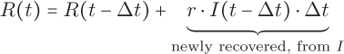
Since no one has yet recovered on day 0, we set the initial condition to be R(0) = 0.
Next, we will consider the difference equation for S(t). The size of the susceptible population only decreases by the number of newly infected people. This decrease depends on the number of susceptible people, the number of infected people with whom they can make contact, and the rate at which these potential interactions produce a new infection. The number of possible interactions between susceptible and infected individuals at time t – Δt is simply their product: S(t – Δt) · I(t – Δt). If we let d represent the rate at which these interactions produce an infection, then our difference equation is

Reflection 4.29 What factors might affect the infection rate in a real outbreak?
If N is the total size of our population, then the initial condition is S(0) = N – 1 because we will start with one infected person, leaving N – 1 who are susceptible.
The difference equation for the infected group depends on the number of susceptible people who have become newly infected and the number of infected people who are newly recovered. These numbers are precisely the number leaving the susceptible group and the number entering the recovered group, respectively. We can simply copy those from the equations above.

Since we are starting with one infected person, we set I(0) = 1.
The program below is a “skeleton” for implementing this model with a recovery rate r = 0.25 and an infection rate d = 0.0004. These rates imply that the average infection lasts 1/r = 4 days and there is a 0.04% chance that an encounter between a susceptible person and an infected person will occur and result in a new infection. The program also demonstrates how to plot and label several curves in the same figure, and display a legend. We leave the implementation of the difference equations in the loop as an exercise.
import matplotlib.pyplot as pyplot

def SIR(population, days, dt):
    """Simulates the SIR model of infectious disease and
       plots the population sizes over time.

    Parameters:
        population: the population size
        days: number of days to simulate
        dt: the value of "Delta t" in the simulation
            (fraction of a day)

    Return value: None
    """

    susceptible = population - 1  # susceptible count = S(t)
    infected = 1.0                # infected count = I(t)
    recovered = 0.0               # recovered count = R(t)
    recRate = 0.25                # recovery rate r
    infRate = 0.0004              # infection rate d
    SList = [susceptible]
    IList = [infected]
    RList = [recovered]
    timeList = [0]

    # Loop using the difference equations goes here.

    pyplot.plot(timeList, SList, label = 'Susceptible')
    pyplot.plot(timeList, IList, label = 'Infected')
    pyplot.plot(timeList, RList, label = 'Recovered')
    pyplot.legend(loc = 'center right')
    pyplot.xlabel('Days')
    pyplot.ylabel('Individuals')
    pyplot.show()
Figure 4.7 shows the output of the model with 2,200 individuals (students at a small college, perhaps?) over 30 days. We can see that the infection peaks after about 2 weeks, then decreases steadily. After 30 days, the virus is just about gone, with only about 40 people still infected. We also notice that not everyone is infected after 30 days; about 80 people are still healthy.
Reflection 4.30 Look at the relationships among the three population sizes over time in Figure 4.7. How do the sizes of the susceptible and recovered populations cause the decline of the affected population after the second week? What other relationships do you notice?
When we are implementing a coupled model, we need to be careful to compute the change in each population size based on population sizes from the previous iteration rather than population sizes previously computed in this iteration. Therefore, we need to compute all of the changes in population sizes for time t, denoted ΔR(t), ΔS(t) and ΔI(t), based on the previous population sizes, before we update the new population sizes in each iteration. In other words, in each iteration, we first compute

ΔR(t)=r·I(t−Δt)·Δt,ΔS(t)=d·S(t−Δt)·I(t−Δt)·Δt,andΔI(t)=ΔS(t)−ΔR(t).
Then, we use these values to update the new population sizes:
R(t)=R(t−Δt)+ΔR(t),S(t)=S(t−Δt)−ΔS(t),andI(t)=I(t−Δt)+ΔI(t).
Interestingly, the SIR model can also be used to model the diffusion of ideas, fads, or memes in a population. A “contagious” idea starts with a small group of people and can “infect” others over time. As more people adopt the idea, it spreads more quickly because there are more potential interactions between those who have adopted the idea and those who have not. Eventually, people move on to other things and forget about the idea, thereby “recovering.”
Exercises
Write a function for each of the following problems.
4.4.1. Suppose we have a pair of rabbits, one male and one female. Female rabbits are mature and can first mate when they are only one month old, and have a gestation period of one month. Suppose that every mature female rabbit mates every month and produces exactly one male and one female offspring one month later. No rabbit ever dies.
(a) Write a difference equation R(m) representing the number of female rabbits at the end of each month. (Note that this is a discrete model; there are no Δt’s.) Start with the first month and compute successive months until you see a pattern. Don’t forget the initial condition(s). To get you started:
• R(0) = 1, the original pair
• R(1) = 1, the original pair now one month old
• R(2) = 2, the original pair plus a newborn pair
• R(3) = 3, the original pair plus a newborn pair plus a one-month-old pair
• R(4) = 5, the pairs from the previous generation plus two newborn pairs
⋮
• R(m) = ?
(b) Write a function
rabbits(months)
that uses your difference equation from part (a) to compute and return the number of rabbits after the given number of months. Your function should also plot the population growth using matplotlib. (The sequence of numbers generated in this problem is called the Fibonacci sequence.)
4.4.2. Consider Exercise 4.1.37, but now assume that a bacteria colony grows continuously with a growth rate of 0.1 Δt per small fraction Δt of an hour.
- Write a difference equation for B(t), the size of the bacteria colony, using Δt’s to approximately model continuous growth.
- Write a function
bacteria(population, dt, days)
that uses your difference equation from part (a) compute and return the number of bacteria in the colony after the given number of
days. The other parameters,populationanddt, are the initial size of the colony and the step size (Δt), respectively. Your function should also plot the population growth usingmatplotlib.
4.4.3. Radioactive elements like carbon-14 are normally described by their half-life, the time required for a quantity of the element to decay to half its original quantity. Write a function
halflifeC14(originalAmount, dt)
that computes the half-life of carbon-14. Your function will need to simulate radioactive decay until the amount is equal to half of originalAmount.
The known half-life of carbon-14 is 5, 730 ± 40 years. How close does this approximation come? Try it with different values of dt.
4.4.4. Finding the half-life of carbon-14 is a special case of radiocarbon dating. When an organic artifact is dated with radiocarbon dating, the fraction of extant carbon-14 is found relative to the content in the atmosphere. Let’s say that the fraction in an ancient piece of parchment is found to be 70%. Then, to find the age of the artifact, we can use a generalized version of halflifeC14 that iterates while amount > originalAmount * 0.7. Show how to generalize the halflifeC14 function in the previous exercise by writing a new function
carbonDate(originalAmount, fractionRemaining, dt)
that returns the age of an artifact with the given fraction of carbon-14 remaining. Use this function to find the approximate age of the parchment.
4.4.5. Complete the implementation of the SIR simulation. Compare your results to Figure 4.7 to check your work.
4.4.6. Run your implementation of the SIR model for longer periods of time than that shown in Figure 4.7. Given enough time, will everyone become infected?
4.4.7. Suppose that enough people have been vaccinated that the infection rate is cut in half. What effect do these vaccinations have?
4.4.8. The SIS model represents an infection that does not result in immunity. In other words, there is no “recovered” population; people who have recovered re-enter the “susceptible” population.
- Write difference equations for this model.
- Copy and then modify the
SIRfunction (renaming itSIS) so that it implements your difference equations. - Run your function with the same parameters that we used for the SIR model. What do you notice? Explain the results.
4.4.9. Suppose there are two predator species that compete for the same prey, but do not directly harm each other. We might expect that, if the supply of prey was low and members of one species were more efficient hunters, then this would have a negative impact on the health of the other species. This can be modeled through the following pair of difference equations. P(t) and Q(t) represent the populations of predator species 1 and 2, respectively, at time t.
P(t)=P(t−Δt)+bP·P(t−Δt)·Δt−dP·P(t−Δt)·Q(t−Δt)·(Δt)Q(t)=Q(t−Δt)+bQ·Q(t−Δt)·Δt−dQ·P(t−Δt)·Q(t−Δt)·(Δt)
The initial conditions are P(0) = p and Q(0) = q, where p and q represent the initial population sizes of the first and second predator species, respectively. The values bP and dP are the birth rate and death rates (or, more formally, proportionality constants) of the first predator species, and the values bQ and dQ are the birth rate and death rate for the second predator species. In the first equation, the term bP · P(t – Δt) represents the net number of births per month for the first predator species, and the term dP · P(t – Δt) · Q(t – Δt) represents the number of deaths per month. Notice that this term is dependent on the sizes of both populations: P(t – Δt) · Q(t – Δt) is the number of possible (indirect) competitions between individuals for food and dP is the rate at which one of these competitions results in a death (from starvation) in the first predator species.
This type of model is known as indirect, exploitative competition because the two predator species do not directly compete with each other (i.e., eat each other), but they do compete indirectly by exploiting a common food supply.
Write a function
compete(pop1, pop2, birth1, birth2, death1, death2, years, dt)
that implements this model for a generalized indirect competition scenario, plotting the sizes of the two populations over time. Run your program using
p = 21 and q = 26
bP = 1.0 and dP = 0.2; bQ = 1.02 and dQ = 0.25
dt = 0.001; 6 years
and explain the results. Here is a “skeleton” of the function to get you started.
def compete(pop1, pop2, birth1, birth2, death1, death2, years, dt):
    """ YOUR DOCSTRING HERE """

    pop1List = [pop1]
    pop2List = [pop2]
    timeList = [0]
    for step in range(1, int(years / dt) + 1):
        # YOUR CODE GOES HERE

    pyplot.plot(timeList, pop1List, label = 'Population 1')
    pyplot.plot(timeList, pop2List, label = 'Population 2')
    pyplot.legend()
    pyplot.xlabel('Years')
    pyplot.ylabel('Individuals')
    pyplot.show()
*4.5 NUMERICAL ANALYSIS
Accumulator algorithms are also used in the natural and social sciences to approximate the values of common mathematical constants, and to numerically compute values and roots of complicated functions that cannot be solved mathematically. In this section, we will discuss a few relatively simple examples from this field of mathematics and computer science, known as numerical analysis.
The harmonic series
Suppose we have an ant that starts walking from one end of a 1 meter long rubber rope. During the first minute, the ant walks 10 cm. At the end of the first minute, we stretch the rubber rope uniformly by 1 meter, so it is now 2 meters long. During the next minute, the ant walks another 10 cm, and then we stretch the rope again by 1 meter. If we continue this process indefinitely, will the ant ever reach the other end of the rope? If it does, how long will it take?
The answer lies in counting what fraction of the rope the ant traverses in each minute. During the first minute, the ant walks 1/10 of the distance to the end of the rope. After stretching, the ant has still traversed 1/10 of the distance because the portion of the rope on which the ant walked was doubled along with the rest of the rope. However, in the second minute, the ant’s 10 cm stroll only covers 10/200 = 1/20 of the entire distance. Therefore, after 2 minutes, the ant has covered 1/10 + 1/20 of the rope. During the third minute, the rope is 3 m long, so the ant covers only 10/300 = 1/30 of the distance. This pattern continues, so our problem boils down to whether the following sum ever reaches 1.
110+120+130+…=110(1+12+13+…)
Naturally, we can answer this question using an accumulator. But how do we add these fractional terms? In Exercise 4.1.25, you may have computed 1 + 2 + 3 + . . . + n:
def sum(n):
    total = 0
    for number in range(1, n + 1):
        total = total + number
    return total
In each iteration of this for loop, we add the value of number to the accumulator variable total. Since number is assigned the values 1, 2, 3, . . ., n, total has the sum of these values after the loop. To compute the fraction of the rope traveled by the ant, we can modify this function to add 1 / number in each iteration instead, and then multiply the result by 1/10:
def ant(n):
    """Simulates the "ant on a rubber rope" problem.  The rope
    is initially 1 m long and the ant walks 10 cm each minute.

    Parameter:
        n: the number of minutes the ant walks

    Return value:
        fraction of the rope traveled by the ant in n minutes
    """

    total = 0
    for number in range(1, n + 1):
        total = total + (1 / number)
    return total * 0.1
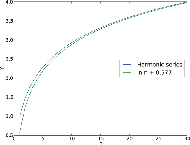
To answer our question with this function, we need to try several values of n to see if we can find a sufficiently high value for which the sum exceeds 1. If we find such a value, then we need to work with smaller values until we find the value of n for which the sum first reaches or exceeds 1.
Reflection 4.31 Using at most 5 calls to the ant function, find a range of minutes that answers the question.
For example, ant(100) returns about 0.52, ant(1000) returns about 0.75, ant(10000) returns about 0.98, and ant(15000) returns about 1.02. So the ant will reach the other end of the rope after 10,000–15,000 minutes. As cumbersome as that was, continuing it to find the exact number of minutes required would be far worse.
Reflection 4.32 How would we write a function to find when the ant first reaches or exceeds the end of the rope? (Hint: this is similar to the carbon-14 half-life problem.) We will leave the answer as an exercise.
This infinite version of the sum that we computed in our loop,
1+12+13+…,
is called the harmonic series and each finite sum
Hn=1+12+13+…+1n
is called the nth harmonic number. (Mathematically, the ant reaches the other end of the rope because the harmonic series diverges, that is, its partial sums increase forever.) The harmonic series can be used to approximate the natural logarithm (ln) function. For sufficiently large values of n,
Hn=1+12+13+…+1n≈In n+0.577.
This is illustrated in Figure 4.8 for only small values of n. Notice how the approximation improves as n increases.
Reflection 4.33 Knowing that Hn ≈ ln n + 0.577, how can you approximate how long until the ant will reach the end of the rope if it walks only 1 cm each minute?
To answer this question, we want to find n such that
100 = ln n + 0.577
since the ant’s first step is not 1/100 of the total distance. This is the same as
e100–0.577 = n.
In Python, we can find the answer with math.exp(100 - 0.577), which gives about 1.5 × 1043 minutes, a long time indeed.
Approximating π
The value π is probably the most famous mathematical constant. There have been many infinite series found over the past 500 years that can be used to approximate π. One of the most famous is known as the Leibniz series, named after Gottfried Leibniz, the co-inventor of calculus:
π=4(1−13+15−17+…)
Like the harmonic series approximation of the natural logarithm, the more terms we compute of this series, the closer we get to the true value of π. To compute this sum, we need to identify a pattern in the terms, and relate them to the values of the index variable in a for loop. Then we can fill in the red blank line below with an expression that computes the ith term from the value of the index variable i.
def leibniz(terms):
    """Computes a partial sum of the Leibniz series.

    Parameter:
        terms: the number of terms to add

    Return value:
        the sum of the given number of terms
    """

    sum = 0
    for i in range(terms):
        sum = sum + ___________
    pi = sum * 4
    return pi
To find the pattern, we can write down the values of the index variable next to the values in the series to identify a relationship:

Ignoring the alternating signs for a moment, we can see that the absolute value of the ith term is
12i+1.
To alternate the signs, we use the fact that –1 raised to an even power is 1, while –1 raised to an odd power is –1. Since the even terms are positive and odd terms are negative, the final expression for the i term is
(−1)i·12i+1.
Therefore, the red assignment statement in our leibniz function should be
sum = sum + (-1) ** i / (2 * i + 1)
Reflection 4.34 Call the completed leibniz function with a series of increasing arguments. What do you notice about how the values converge to π?
By examining several values of the function, you might notice that they alternate between being greater and less than the actual value of π. Figure 4.9 illustrates this.
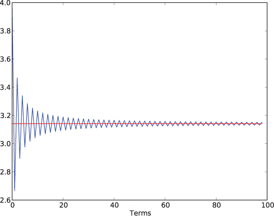
Approximating square roots
The square root function (√n

Here, n is the value whose square root we want. The approximation of √n
Similar to our previous examples, we can compute successive values of the difference equation using iteration. In this case, each value is computed from the previous value according to the formula above. If we let the variable name x represent a term in the difference equation, then we can compute the kth term with the following simple function:
def sqrt(n, k):
    """Approximates the square root of n with k iterations
       of the Babylonian method.

    Parameters:
        n: the number to take the square root of
        k: number of iterations

    Return value:
        the approximate square root of n
    """

    x = 1.0
    for index in range(k):
        x = 0.5 * (x + n / x)
    return x
Reflection 4.35 Call the function above to approximate √10math.sqrt function?
Exercises
4.5.1. Recall Reflection 4.32: How would we write a function to find when the ant first reaches or exceeds the end of the rope? (Hint: this is similar to the carbon-14 half-life problem.)
- Write a function to answer this question.
- How long does it take for the ant to traverse the entire rope?
- If the ant walks 5 cm each minute, how long does it take to reach the other end?
4.5.2. Augment the ant function so that it also produces the plot in Figure 4.8.
4.5.3. The value e (Euler’s number, the base of the natural logarithm) is equal to the infinite sum
e=1+11!+12!+13!+…
Write a function
e(n)
that approximates the value of e by computing and returning the value of n terms of this sum. For example, calling e(4) should return the value 1+1/1+1/2+1/6 ≈ 2.667. Your function should call the factorial function you wrote for Exercise 4.1.29 to aid in the computation.
4.5.4. Calling the factorial function repeatedly in the function you wrote for the previous problem is very inefficient because many of the same arithmetic operations are being performed repeatedly. Explain where this is happening.
4.5.5. To avoid the problems suggested by the previous exercise, rewrite the function from Exercise 4.5.3 without calling the factorial function.
4.5.6. Rather than specifying the number of iterations in advance, numerical algorithms usually iterate until the absolute value of the current term is sufficiently small. At this point, we assume the approximation is “good enough.” Rewrite the leibniz function so that it iterates while the absolute value of the current term is greater than 10–6.
4.5.7. Similar to the previous exercise, rewrite the sqrt function so that it iterates while the absolute value of the difference between the current and previous values of x is greater than 10–15.
4.5.8. The following expression, discovered in the 14th century by Indian mathematician Madhava of Sangamagrama, is another way to compute π.
π=√12(1−13·3+15·32−17·33+…)
Write a function
approxPi(n)
that computes n terms of this expression to approximate π. For example, approxPi(3) should return the value
√12(1−13·3+15·32)≈√12(1−0.111+0.022)≈3.156.
To determine the pattern in the sequence of terms, consider this table:

What is the term for a general value of i?
4.5.9. The Wallis product, named after 17th century English mathematician John Wallis, is an infinite product that converges to π:
π=2(21·23·43·45·65·67. …)
Write a function
wallis(terms)
that computes the given number of terms in the Wallis product. Hint: Consider the terms in pairs and find an expression for each pair. Then iterate over the number of pairs needed to flesh out the required number of terms. You may assume that terms is even.
4.5.10. The Nilakantha series, named after Nilakantha Somayaji, a 15th century Indian mathematician, is another infinite series for π:
π=3+42·3·4−44·5·6+46·7·8−48·9·10+…
Write a function
nilakantha(terms)
that computes the given number of terms in the Nilakantha series.
4.5.11. The following infinite product was discovered by François Viète, a 16th century French mathematician:
π=2·2√2·2√2+√2·2√2+√2+√2·2√2+√2+√2+√2…
Write a function
viete(terms)
that computes the given number of terms in the Viète’s product. (Look at the pattern carefully; it is not as hard as it looks if you base the denominator in each term on the denominator of the previous term.)
4.6 SUMMING UP
Although we have solved a variety of different problems in this chapter, almost all of the functions that we have designed have the same basic format:
def accumulator( ___________):
    sum = _________              # initialize the accumulator
    for index in range(_______): # iterate some number of times
        sum = sum + ________     # add something to the accumulator
    return sum                   # return final accumulator value
The functions we designed differ primarily in what is added to the accumulator (the red statement) in each iteration of the loop. Let’s look at three of these functions in particular: the pond function from Page 119, the countLinks function from Page 123, and the solution to Exercise 4.1.27 from Page 134, shown below.
def growth(finalAge):
    height = 95
    for age in range(4, finalAge + 1):
        height = height + 6
    return height
In the growth function, a constant value is added to the accumulator in each iteration:

Figure 4.10 An illustration of linear, quadratic, and exponential growth. The curves are generated by accumulators adding 6, the index variable, and 1.08 times the accumulator, respectively, in each iteration.
height = height + 6
In the countLinks function, the value of the index variable, minus one, is added to the accumulator:
newLinks = node - 1
totalLinks = totalLinks + newLinks
And in the pond function, a factor of the accumulator itself is added in each iteration:
population = population + 0.08 * population # ignoring "- 1500"
(To simplify things, we will ignore the subtraction present in the original program.)
These three types of accumulators grow in three different ways. Adding a constant value to the accumulator in each iteration, as in the growth function, results in a final sum that is equal to the number of iterations times the constant value. In other words, if the initial value is a, the constant added value is c, and the number of iterations is n, the final value of the accumulator is a + cn. (In the growth function, a = 95 and c = 6, so the final sum is 95 + 6n.) As n increases, cn increases by a constant amount. This is called linear growth, and is illustrated by the blue line in Figure 4.10.
Adding the value of the index variable to the accumulator, as in the countLinks function, results in much faster growth. In the countLinks function, the final value
There are a few nice tricks to figure out the value of the sum
1 + 2 + 3 + . . . + (n – 2) + (n – 1) + n
for any positive integer n. The first technique is to add the numbers in the sum from the outside in. Notice that the sum of the first and last numbers is n + 1. Then, coming in one position from both the left and right, we find that (n – 1) + 2 = n + 1 as well. Next, (n – 2) + 3 = n + 1. This pattern will obviously continue, as we are subtracting 1 from the number on the left and adding 1 to the number on the right. In total, there is one instance of n + 1 for every two terms in the sum, for a total of n/2 instances of n + 1. Therefore, the sum is
1+2+3+…+(n−2)+(n−1)+n=n2(n+1)=n(n+1)2.
For example, 1+2+3 +. . .+8 = (8·9)/2 = 36 and 1+2+3+. . .+1000 = (1000·1001)/2 = 500, 500.
The second technique to derive this result is more visual. Depict each number in the sum as a column of circles, as shown on the left below with n = 8.

The first column has n = 8 circles, the second has n – 1 = 7, etc. So the total number of circles in this triangle is equal to the value we are seeking. Now make an exact duplicate of this triangle, and place its mirror image to the right of the original triangle, as shown on the right above. The resulting rectangle has n rows and n + 1 columns, so there are a total of n(n + 1) circles. Since the number of circles in this rectangle is exactly twice the number in the original triangle, the number of circles in the original triangle is n(n + 1)/2. Based on this representation, numbers like 36 and 500, 500 that are sums of this form are called triangular numbers.
of the accumulator is
1 + 2 + 3 + . . . + (n – 1)
which is equal to
12·n·(n−1)=n2−n2.
Box 4.2 explains two clever ways to derive this result. Since this sum is proportional to n2, we say that it exhibits quadratic growth, as shown by the red curve in Figure 4.10. This sum is actually quite handy to know, and it will surface again in Chapter 11.
Finally, adding a factor of the accumulator to itself in each iteration, as in the pond function, results in even faster growth. In the pond function, if we add 0.08 * population to population in each iteration, the accumulator variable will be equal to the initial value of population times 1.08n at the end of n iterations of the loop. For this reason, we call this exponential growth, which is illustrated by the green curve in Figure 4.10. Notice that, as n gets larger, exponential growth quickly outpaces the other two curves, even when the number we are raising n to is small, like 1.08.
So although all accumulator algorithms look more or less alike, the effects of the accumulators can be strikingly different. Understanding the relative rates of these different types of growth is quite important in a variety of fields, not just computer science. For example, mistaking an exponentially growing epidemic for a linearly growing one can be a life or death mistake!
These classes of growth can also be applied to the efficiency of algorithms, as we will see in in later chapters. In this case, n would represent the size of the input and the y-axis would represent the number of elementary steps required by the algorithm to compute the corresponding output.
Exercises
4.6.1. Decide whether each of the following accumulators exhibits linear, quadratic, or exponential growth.
(a)
sum = 0
     for index in range(n):
         sum = sum + index * 2
(b)
sum = 10
     for index in range(n):
         sum = sum + index / 2
(c)
sum = 1
     for index in range(n):
         sum = sum + sum
(d)
sum = 0
     for index in range(n):
         sum = sum + 1.2 * sum
(e)
sum = 0
     for index in range(n):
         sum = sum + 0.01
(f)
sum = 10
     for index in range(n):
         sum = 1.2 * sum
4.6.2. Look at Figure 4.10. For values of n less than about 80, the fast-growing exponential curve is actually below the other two. Explain why.
4.6.3. Write a program to generate Figure 4.10.
4.7 FURTHER DISCOVERY
The epigraph of this chapter is from a TED talk given by Stephen Hawking in 2008. You can watch it yourself at
www.ted.com/talks/stephen_hawking_asks_big_questions_about_the_universe.
If you are interested in learning more about population dynamics models, and computational modeling in general, a great source is Introduction to Computational Science [52] by Angela Shiflet and George Shiflet.
4.8 PROJECTS
Project 4.1 Parasitic relationships
For this project, we assume that you have read the material on discrete difference equations on Pages 145–146 of Section 4.4.
A parasite is an organism that lives either on or inside another organism for part of its life. A parasitoid is a parasitic organism that eventually kills its host. A parasitoid insect infects a host insect by laying eggs inside it then, when these eggs later hatch into larvae, they feed on the live host. (Cool, huh?) When the host eventually dies, the parasitoid adults emerge from the host body.
The Nicholson-Bailey model, first proposed by Alexander Nicholson and Victor Bailey in 1935 [36], is a pair of difference equations that attempt to simulate the relative population sizes of parasitoids and their hosts. We represent the size of the host population in year t with H(t) and the size of the parasitoid population in year t with P(t). Then the difference equations describing this model are
H(t)=r·H(t−1)·e−aP(t−1)P(t)=c·H(t−1)·(1−e−aP(t−1))
where
r is the average number of surviving offspring from an uninfected host,
c is the average number of eggs that hatch inside a single host, and
a is a scaling factor describing the searching efficiency or search area of the parasitoids (higher is more efficient).
The value (1 – e–aP(t–1)) is the probability that a host is infected when there are P(t – 1) parasitoids, where e is Euler’s number (the base of the natural logarithm). Therefore,
H(t – 1) · (1 – e–aP(t–1))
is the number of hosts that are infected during year t – 1. Multiplying this by c gives us P(t), the number of new parasitoids hatching in year t. Notice that the probability of infection grows exponentially as the size of the parasitoid population grows. A higher value of a also increases the probability of infection.
Question 4.1.1 Similarly explain the meaning of the difference equation for H(t) · (e–aP(t–1) is the probability that a host is not infected.)
Part 1: Implement the model
To implement this model, write a function
NB(hostPop, paraPop, r, c, a, years)
that uses these difference equations to plot both population sizes over time. Your function should plot these values in two different ways (resulting in two different plots). First, plot the host population size on the x-axis and the parasitoid population size on the y-axis. So each point represents the two population sizes in a particular year. Second, plot both population sizes on the y-axis, with time on the x-axis. To show both population sizes on the same plot, call the pyplot.plot function for each population list before calling pyplot.show. To label each line and include a legend, see the end of Section 4.2.
Question 4.1.2 Write a main function that calls your NB function to simulate initial populations of 24 hosts and 12 parasitoids for 35 years. Use values of r = 2, c = 1, and a = 0.056. Describe and interpret the results.
Question 4.1.3 Run the simulation again with the same parameters, but this time assign a to be -math.log(0.5) / paraPop. (This is a = – ln 0.5/12 ≈ 0.058, just slightly above the original value of a.) What do you observe?
Question 4.1.4 Run the simulation again with the same parameters, but this time assign a = 0.06. What do you observe?
Question 4.1.5 Based on these three simulations, what can you say about this model and its sensitivity to the value of a?
Part 2: Constrained growth
An updated Nicholson-Bailey model incorporates a carrying capacity that keeps the host population under control. The carrying capacity of an ecosystem is the maximum number of organisms that the ecosystem can support at any particular time. If the population size exceeds the carrying capacity, there are not enough resources to support the entire population, so some individuals do not survive.
In this revised model, P(t) is the same, but H(t) is modified to be
H(t) = H(t–1) · e–aP(t–1) · er(1–H(t–1)/K)
where K is the carrying capacity. In this new difference equation, the average number of surviving host offspring, formerly r, is now represented by
er(1–H(t–1)/K).
Notice that, when the number of hosts H(t – 1) equals the carrying capacity K, the exponent equals zero. So the number of surviving host offspring is e0 = 1. In general, as the number of hosts H(t – 1) gets closer to the carrying capacity K, the exponent gets smaller and the value of the expression above gets closer to 1. At the other extreme, when H(t – 1) is close to 0, the expression is close to er. So, overall, the number of surviving offspring varies between 1 and er, depending on how close H(t – 1) comes to the carrying capacity.
Write a function
NB_CC(hostPop, paraPop, r, c, a, K, years)
that implements this modified model and generates the same plots as the previous function.
Question 4.1.6 Call your NB_CC function to simulate initial populations of 24 hosts and 12 parasitoids for 35 years. Use values of r = 1.5, c = 1, a = 0.056, and K = 40. Describe and interpret the results.
Question 4.1.7 Run your simulation with all three values of a that we used in Part 1. How do these results differ from the prior simulation?
Project 4.2 Financial calculators
In this project, you will write three calculators to help someone (maybe you) plan for your financial future.
Part 1: How long will it take to repay my college loans?
Your first calculator will compare the amount of time it takes to repay student loans with two different monthly payment amounts. Your main program will need to prompt for
the student loan balance at the time repayment begins
the nominal annual interest rate (the monthly rate times twelve)
two monthly payment amounts
Then write a function
comparePayoffs(amount, rate, monthly1, monthly2)
that computes the number of months required to pay off the loan with each monthly payment amount. The interest on the loan balance should compound monthly at a rate of rate / 100 / 12. Your function should also plot the loan balances, with each payment amount, over time until both balances reach zero. Then it should print the length of both repayment periods and how much sooner the loan will be paid off if the higher monthly payment is chosen. For example, your output might look like this:
Initial balance: 60000
Nominal annual percentage rate: 5
Monthly payment 1: 500
Monthly payment 2: 750

If you pay $500.00 per month, the repayment period will be 13 years
and 11 months.
If you pay $750.00 per month, the repayment period will be 8 years
and 2 months.
If you pay $250.00 more per month, you will repay the loan 5 years
and 9 months earlier.
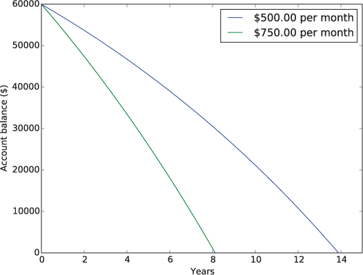
Question 4.2.1 How long would it take to pay off $20,000 in student loans with a 4% interest rate if you paid $100 per month? Approximately how much would you have to pay per month to pay off the loan in ten years?
Question 4.2.2 If you run your program to determine how long it would take to pay off the same loan if you paid only $50 per month, you should encounter a problem. What is it?
Part 2: How much will I have for retirement?
Your second calculator will compare the retirement nest eggs that result from making two different monthly investments in a retirement fund. Your program should prompt for the following inputs:
the initial balance in the retirement account
the current age of the investor
the desired retirement age of the investor
the expected nominal annual rate of return on the investment
two monthly investment amounts
Then write a function
compareInvestments(balance, age, retireAge, rate, monthly1, monthly2)
that computes the final balance in the retirement account, for each monthly investment, when the investor reaches his or her retirement age. The interest on the current balance should compound monthly at a rate of rate / 100 / 12. The function should plot the growth of the retirement account balance for both monthly investment amounts, and then print the two final balances along with the additional amount that results from the higher monthly investment. For example, your output might look like this:
Initial balance: 1000
Current age: 20
Retirement age: 70
Nominal annual percentage rate of return: 4.2
Monthly investment 1: 100
Monthly investment 2: 150

The final balance from investing $100.00 per month: $212030.11.
The final balance from investing $150.00 per month: $313977.02.
If you invest $50.00 more per month, you will have $101946.91 more at
 retirement.

Question 4.2.3 Suppose you are 30 and, after working for a few years, have managed to save $6,000 for retirement. If you continue to invest $200 per month, how much will you have when you retire at age 72 if your investment grows 3% per year? How much more will you have if you invest $50 more per month?
Part 3: How long will my retirement savings last?
Your third calculator will initially perform the same computation as your previous calculator, but with only one monthly investment amount. After it computes the final balance in the account, it will estimate how long that nest egg will last into retirement. Your program will need to prompt for the same values as above (but only one monthly investment amount), plus the percentage of the final balance the investor plans to withdraw in the first year after retirement. Then write a function
retirement(amount, age, retireAge, rate, monthly, percentWithdraw)
that adds the monthly investment amount to the balance in the retirement account until the investor reaches his or her retirement age, and then, after retirement age, withdraws a monthly amount. In the first month after retirement, this amount should be one-twelth of percentWithdraw of the current balance. For every month thereafter, the withdrawal amount should increase according to the rate of inflation, assumed to be 3% annually. Every month, the interest on the current balance should compound at a rate of rate / 100 / 12. The function should plot the retirement account balance over time, and then print the age at which the retirement funds run out. For example, your program output might look like this:
Initial balance: 10000
Current age: 20
Retirement age: 70
Annual percentage rate of return: 4.2
Monthly investment: 100
Annual withdrawal % at retirement: 4

Your savings will last until you are 99 years and 10 months old.
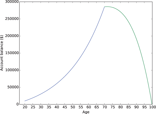
Question 4.2.4 How long will your retirement savings last if you follow the plan outlined in Question 4.2 (investing $200 per month) and withdraw 4% at retirement?
*Project 4.3 Market penetration
For this project, we assume that you have read Section 4.4.
In this project, you will write a program that simulates the adoption of a new product in a market over time (i.e., the product’s “market penetration”) using a difference equation developed by marketing researcher Frank Bass in 1969 [4]. The Bass diffusion model assumes that there is one product and a fixed population of N eventual adopters of that product. In the difference equation, A(t) is the fraction (between 0 and 1) of the population that has adopted the new product t weeks after the product launch. Like the difference equations in Section 4.4, the value of A(t) will depend on the value of A(t – Δt), the fraction of the population that had adopted the product at the previous time step, t – Δt. Since t is measured in weeks, Δt is some fraction of a week. The rate of product adoption depends on two factors.
The segment of the population that has not yet adopted the product adopts it at a constant adoption rate of r due to chance alone. By the definition of A(t), the fraction of the population that had adopted the product at the previous time step is A(t – Δt). Therefore, the fraction of the population that had not yet adopted the product at the previous time step is 1 – A(t – Δt). So the fraction of new adopters during week t from this constant adoption rate is
r · (1 – A(t – Δt)) · Δt.
Second, the rate of adoption is affected by word of mouth within the population. Members of the population who have already adopted the product can influence those who have not. The more adopters there are, the more potential interactions exist between adopters and non-adopters, which boosts the adoption rate. The fraction of all potential interactions that are between adopters and non-adopters in the previous time step is
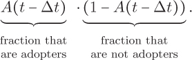
The fraction of these interactions that result in a new adoption during one week is called the social contagion. We will denote the social contagion by s. So the fraction of new adopters due to social contagion during the time step ending at week t is
s · A(t – Δt) · (1 – A(t – Δt)) · Δt.
The social contagion measures how successfully adopters are able to convince non-adopters that they should adopt the product. At the extremes, if s = 1, then every interaction between a non-adopter and an adopter results in the non-adopter adopting the product. On the other hand, if s = 0, then the current adopters cannot convince any non-adopters to adopt the product.
Putting these two parts together, the difference equation for the Bass diffusion model is

Part 1: Implement the Bass diffusion model
To implement the Bass diffusion model, write a function
productDiffusion(chanceAdoption, socialContagion, weeks, dt)
The parameters chanceAdoption and socialContagion are the values of r and s, respectively. The last two parameters give the number of weeks to simulate and the value of Δt to use. Your function should plot two curves, both with time on the x-axis and the proportion of adopters on the y-axis. The first curve is the total fraction of the population that has adopted the product by time t. This is A(t) in the difference equation above. The second curve will be the rate of change of A(t). You can calculate this by the formula
A(t)−A(t−Δt)Δt.
Equivalently, this rate of change can be thought of as the fraction of new adopters at any time step, normalized to a weekly rate, i.e., the fraction of the population added in that time step divided by dt.
Write a program that uses your function to simulate a product launch over 15 weeks, using Δt= 0.01. For this product launch, we will expect that adoption of the product will move slowly without a social effect, but that social contagion will have a significant impact. To model these assumptions, use r = 0.002 and s = 1.03.
Question 4.3.1 Describe the picture and explain the pattern of new adoptions and the resulting pattern of total adoptions over the 15-week launch.
Question 4.3.2 Now make r very small but leave s the same (r = 0.00001, s = 1.03), and answer the same question. What kind of market does this represent?
Question 4.3.3 Now set r to be 100 times its original value and s to be zero (r = 0.2, s = 0), and answer the first question again. What kind of market does this represent?
Part 2: Influentials and imitators
In a real marketplace, some adopters are more influential than others. Therefore, to be more realistic, we will now partition the entire population into two groups called influentials and imitators [56]. Influentials are only influenced by other influentials, while imitators can be influenced by either group. The numbers of influentials and imitators in the population are NA and NB, respectively, so the total population size is N = NA + NB. We will let A(t) now represent the fraction of the influential population that has adopted the product at time t and let B(t) represent the fraction of the imitator population that has adopted the product at time t.
The adoption rate of the influentials follows the same difference equation as before, except that we will denote the adoption rate and social contagion for the influentials with rA and sA.
A(t) = A(t – Δt) + rA · (1 – A(t – Δt)) · Δt + sA · A(t – Δt) · (1 – A(t – Δt)) · Δt
The adoption rate of the imitators will be different because they value the opinions of both influentials and other imitators. Let rB and sB represent the adoption rate and social contagion for the imitators. Another parameter, w (between 0 and 1), will indicate how much the imitators value the opinions of the influentials over the other imitators. At the extremes, w = 1 means that the imitators are influenced heavily by influentials and not at all by other imitators. On the other hand, w = 0 means that they are not at all influenced by influentials, but are in uenced by imitators. We will break the difference equation for B(t) into three parts.
First, there is a constant rate of adoptions from among the imitators that have not yet adopted, just like the first part of the difference equation for A(t):
rB · (1 – B(t – Δt)) · Δt
Second, there is a fraction of the imitators who have not yet adopted who will be influenced to adopt, through social contagion, by influential adopters.
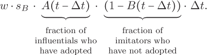
Recall from above that w is the extent to which imitators are more likely to be influenced by influentials than other imitators.
Third, there is a fraction of the imitators who have not yet adopted who will be influenced to adopt, through social contagion, by other imitators who have already adopted.
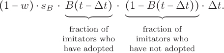
The term 1 – w is the extent to which imitators are likely to be influenced by other imitators, compared to influentials.
Putting these three parts together, we have the difference equation modeling the growth of the fraction of imitators who adopt the product.
B(t)=B(t−Δt)+rB·(1−B(t−Δt))·Δt+w·sB·A(t−Δt)·(1−B(t−Δt))·Δt+(1−w)·sB·B(t−Δt)·(1−B(t−Δt))·Δt
Now write a function
productDiffusion2(inSize, imSize, rIn, sIn, rIm, sIm, weight, weeks, dt)
that implements this product diffusion model with influentials and imitators. The parameters are similar to the previous function (but their names have been shortened). The first two parameters are the sizes of the influential and imitator populations, respectively. The third and fourth parameters are the adoption rate (rA) and social contagion (sA) for the influentials, respectively. The fifth and sixth parameters are the same values (rB and sB) for the imitators. The seventh parameter weight is the value of w. Your function should produce two plots. In the first, plot the new adoptions for each group, and the total new adoptions, over time (as before, normalized by dividing by dt). In the second, plot the total adoptions for each group, and the total adoptions for both groups together, over time. Unlike in the previous function, plot the numbers of adopters in each group rather than the fractions of adopters, so that the different sizes of each population are taken into account. (To do this, just multiply the fraction by the total size of the appropriate population.)
Write a program that uses your function to simulate the same product launch as before, except now there are 600 influentials and 400 imitators in a total population of 1000. The adoption rate and social contagion for the influentials are the same as before (rA = 0.002 and sA = 1.03), but these values are rB = 0 and sB = 0.8 for the imitators. Use a value of w = 0.6, meaning that the imitators value the opinions of the influentials over other imitators.
Question 4.3.4 Describe the picture and explain the pattern of new adoptions and the resulting pattern of total adoptions. Point out any patterns that you find interesting.
Question 4.3.5 Now set w = 0.01 and rerun the simulation. Describe the new picture and explain how and why this changes the results.
*Project 4.4 Wolves and moose
For this project, we assume that you have read Section 4.4.
Predator-prey models are commonly used in biology because they can model a wide range of ecological relationships, e.g., wolves and moose, koala and eucalyptus, or humans and tuna. In the simplest incarnation, the livelihood of a population of predators is dependent solely on the availability of a population of prey. The population of prey, in turn, is kept in check by the predators.
In the 1920’s, Alfred Lotka and Vito Volterra independently introduced the now-famous Lotka-Volterra equations to model predator-prey relationships. The model consists of a pair of related differential equations that describe the sizes of the two populations over time. We will approximate the differential equations with discrete difference equations. Let’s assume that the predators are wolves and the prey are moose. We will represent the sizes of the moose and wolf populations at the end of month t with M(t) and W(t), respectively. The difference equations describing the populations of wolves and moose are:
M(t)=M(t−Δt)+bMM(t−Δt)Δt−dMW(t−Δt)M(t−Δt)ΔtW(t)=W(t−Δt)+bWW(t−Δt)M(t−Δt)Δt−dWW(t−Δt)Δt
where
bM is the moose birth rate (per month)
dM is the moose death rate, or the rate at which a wolf kills a moose that it encounters (per month)
bW is the wolf birth rate, or the moose death rate × how efficiently an eaten moose produces a new wolf (per month)
dW is the wolf death rate (per month)
Let’s look at these equations more closely. In the first equation, the term bM M(t – Δt) Δt represents the net number of moose births in the last time step, in the absence of wolves, and the term dM W(t – Δt) M(t – Δt) Δt represents the number of moose deaths in the last time step. Notice that this term is dependent on both the number of wolves and the number of moose: W(t – Δt) M(t – Δt) is the number of possible wolf-moose encounters and dM Δt is the rate at which a wolf kills a moose that it encounters in a time step of length Δt.
In the second equation, the term bW W(t – Δt) M(t – Δt)Δt represents the number of wolf births per month. Notice that this number is also proportional to both the number of wolves and the number of moose, the idea being that wolves will give birth to more offspring when food is plentiful. As described above, bW is actually based on two quantities, the moose death rate (since wolves have to eat moose to thrive and have offspring) and how efficiently a wolf can use the energy gained by eating a moose to give birth to a new wolf. The term dW W(t – Δt)Δt represents the net number of wolf deaths per month in the absence of moose.
In this project, you will write a program that uses these difference equations to model the dynamic sizes of a population of wolves and a population of moose over time. There are three parts to the project. In the first part, you will use the Lotka-Volterra model to simulate a baseline scenario. In the second part, you will model the effects that hunting the wolves have on the populations. And, in the third part, you will create a more realistic simulation in which the sizes of the populations are limited by the natural resources available in the area.
Part 1: Implement the Lotka-Volterra model
Write a function in Python
PP(preyPop, predPop, dt, months)
that simulates this predator prey model using the difference equations above. The parameters preyPop and predPop are the initial sizes of the prey and predator populations (M(0) and W(0)), respectively, dt (Δt) is the time interval used in the simulation, and months is the number of months (maximum value of t) for which to run the simulation. To cut back on the number of parameters, you can assign constant birth and death rates to local variables inside your function. Start by trying
|
|
|
|
|
|
|
|
Your function should plot, using matplotlib, the sizes of the wolf and moose populations over time, as the simulation progresses. Write a program that calls your PP function to simulate 500 moose and 25 wolves for 5 years with dt = 0.01.
Question 4.4.1 What happens to the sizes of the populations over time? Why do these changes occur?
Part 2: Here come the hunters!
Now suppose the wolves begin to threaten local ranchers’ livestock (in Wyoming, for example) and the ranchers begin killing the wolves. Simulate this effect by increasing the wolf death rate dW.
Question 4.4.2 What is the effect on the moose population?
Question 4.4.3 What would the wolf death rate need to be for the wolf population to die out within five years? Note that the death rate can exceed 1. Try increasing the value of dW slowly and watch what happens. If it seems like you can never kill all the wolves, read on.
Killing off the wolves appears to be impossible because the equations you are using will never let the value reach zero. (Why?) To compensate, we can set either population to zero when it falls below some threshold, say 1.0. (After all, you can’t really have a fraction of a wolf.) To do this, insert the following statements into the body of your for loop after you increment the predator and prey populations, and try answering the previous question again.
if preyPop < 1.0:
    preyPop = 0.0
if predPop < 1.0:
    predPop = 0.0
(Replace preyPop and predPop with the names you use for the current sizes of the populations.) As we will see shortly, the first two statements will assign 0 to preyPop if it is less than 1. The second two statements do the same for predPop.
Part 3: Modeling constrained growth
In the simulation so far, we have assumed that a population can grow without bound. For example, if the wolf population died out, the moose population would grow exponentially. In reality, an ecosystem can only support a limited size population due to constraints on space, food, etc. This limit is known as a carrying capacity. We can model the moose carrying capacity in a simple way by decreasing the moose birth rate proportionally to the size of the moose population. Specifically, let MCC represent the moose population carrying capacity, which is the maximum number of moose the ecosystem can support. Then change the moose birth term bM M(t – Δt)Δt to
bM (1 – M(t – Δt)/MCC)M(t – Δt)Δt.
Notice that now, as the moose population size approaches the carrying capacity, the birth rate slows.
Question 4.4.4 Why does this change cause the moose birth rate to slow as the size of the moose population approaches the carrying capacity?
Implement this change to your simulation, setting the moose carrying capacity to 750, and run it again with the original birth and death rates, with 500 moose and 25 wolves, for 10 years.
Question 4.4.5 How does the result differ from your previous run? What does the result demonstrate? Does the moose population reach its carrying capacity of 750? If not, what birth and/or death rate parameters would need to change to allow this to happen?
Question 4.4.6 Reinstate the original birth and death rates, and introduce hunting again; now what would the wolf death rate need to be for the wolf population to die out within five years?
1MATLAB is a registered trademark of The MathWorks, Inc.
2The probability of a carbon-14 molecule decaying in a very small fraction Δt of a year is k Δ t.