
CHAPTER 5
Forks in the road
When you come to a fork in the road, take it.
Yogi Berra
SO far, our algorithms have been entirely deterministic; they have done the same thing every time we execute them with the same inputs. However, the natural world and its inhabitants (including us) are usually not so predictable. Rather, we consider many natural processes to be, to various degrees, random. For example, the behaviors of crowds and markets often change in unpredictable ways. The genetic “mixing” that occurs in sexual reproduction can be considered a random process because we cannot predict the characteristics of any particular offspring. We can also use the power of random sampling to estimate characteristics of a large population by querying a smaller number of randomly selected individuals.
Most non-random algorithms must also be able to conditionally change course, or select from among a variety of options, in response to input. Indeed, most common desktop applications do nothing unless prompted by a key press or a mouse click. Computer games like racing simulators react to a controller several times a second. The protocols that govern data traffic on the Internet adjust transmission rates continually in response to the perceived level of congestion on the network. In this chapter, we will discover how to design algorithms that can behave differently in response to input, both random and deterministic.
5.1 RANDOM WALKS
Scientists are often interested in simulating random processes to better understand some characteristic of a system. For example, we may wish to estimate the theoretical probability of some genetic abnormality or the expected distance a particle moves in Brownian motion. Algorithms that employ randomness to estimate some value are called Monte Carlo simulations, after the famous casino in Monaco. Monte Carlo simulations repeat a random experiment many, many times, and average over these trials to arrive at a meaningful result; one run of the simulation, due to its random nature, does not carry any significance.
It is customary to represent the interval (i.e., set or range), of real numbers between a and b, including a and b, with the notation [a, b]. In contrast, the set of integers between the integers a and b, including a and b, is denoted [a . . b]. For example, [3, 7] represents every real number greater than or equal to 3 and less than or equal to 7, while [3 . . 7] represents the integers 3, 4, 5, 6, 7.
To denote an interval of real numbers between a and b that does not contain an endpoint a or b, we replace the endpoint’s square bracket with a parenthesis. So [a, b) is the interval of real numbers between a and b that does contain a but does not contain b. Similarly, (a, b] contains b but not a, and (a, b) contains neither a nor b.
In 1827, British Botanist Robert Brown, while observing pollen grains suspended in water under his microscope, witnessed something curious. When the pollen grains burst, they emitted much smaller particles that proceeded to wiggle around randomly. This phenomenon, now called Brownian motion, was caused by the particles’ collisions with the moving water molecules. Brownian motion is now used to describe the motion of any sufficiently small particle (or molecule) in a fluid.
We can model the essence of Brownian motion with a single randomly moving particle in two dimensions. This process is known as a random walk. Random walks are also used to model a wide variety of other phenomena such as markets and the foraging behavior of animals, and to sample large social networks. In this section, we will develop a Monte Carlo simulation of a random walk to discover how far away a randomly moving particle is likely to get in a fixed amount of time.
You may have already modeled a simple random walk in Exercise 3.3.15 by moving a turtle around the screen and choosing a random angle to turn at each step. We will now develop a more restricted version of a random walk in which the particle is forced to move on a two-dimensional grid. At each step, we want the particle to move in one of the four cardinal directions, each with equal probability.
To simulate random processes, we need an algorithm or device that produces random numbers, called a random number generator (RNG). A computer, as described in Chapter 1, cannot implement a true RNG because everything it does is entirely predictable. Therefore, a computer either needs to incorporate a specialized device that can detect and transmit truly random physical events (like subatomic quantum fluctuations) or simulate randomness with a clever algorithm called a pseudorandom number generator (PRNG). A PRNG generates a sequence of numbers that appear to be random although, in reality, they are not.
The Python module named random provides a PRNG in a function named random. The random function returns a pseudorandom number between zero and one, but not including one. For example:
>>> import random
>>> random.random()
0.9699738944412686
(Your output will differ.) It is convenient to refer to the range of real numbers produced by the random function as [0, 1). The square bracket on the left means that 0 is included in the range, and the parenthesis on the right means that 1 is not included in the range. Box 5.1 explains a little more about this so-called interval notation, if it is unfamiliar to you.
To randomly move our particle in one of four cardinal directions, we first use the random function to assign r to be a random value in [0, 1). Then we divide our space of possible random numbers into four equal intervals, and associate a direction with each one.
If r is in [0, 0.25), then move east.
If r is in [0.25, 0.5), then move north.
If r is in [0.5, 0.75), then move west.
If r is in [0.75, 1.0), then move south.
Now let’s write an algorithm to take one step of a random walk. We will save the particle’s (x, y) location in two variables, x and y (also called the particle’s x and y coordinates). To condition each move based on the interval in which r resides, we will use Python’s if statement. An if statement executes a particular sequence of statements only if some condition is true. For example, the following statements assign a pseudorandom value to r, and then implement the first case by incrementing x when r is in [0, 0.25):
x = 0
y = 0
r = random.random()
if r < 0.25:                     # if r < 0.25,
    x = x + 1                    #   move to the east
An if statement is also called a conditional statement because, like the while loops we saw earlier, they make decisions that are conditioned on a Boolean expression. (Unlike while loops, however, an if statement is only executed once.) The Boolean expression in this case, r < 0.25, is true if r is less than 0.25 and false otherwise. If the Boolean expression is true, the statement(s) that are indented beneath the condition are executed. On the other hand, if the Boolean expression is false, the indented statement(s) are skipped, and the statement following the indented statements is executed next.

In the second case, to check whether r is in [0.25, 0.5), we need to check whether r is greater than or equal to 0.25 and whether r is less than 0.5. The meaning of “and” in the previous sentence is identical to the Boolean operator from Section 1.4. In Python, this condition is represented just as you would expect:
r >= 0.25 and r < 0.5
The >= operator is Python’s representation of “greater than or equal to” (≥). It is one of six comparison operators (or relational operators), listed in Table 5.1, some of which have two-character representations in Python. (Note especially that == is used to test for equality. We will discuss these operators further in Section 5.4.) Adding this case to the first case, we now have two if statements:
if r < 0.25:                    # if r < 0.25,
    x = x + 1                   #   move to the east
if r >= 0.25 and r < 0.5:       # if r is in [0.25, 0.5),
    y = y + 1                   #   move to the north
Now if r is assigned a value that is less than 0.25, the condition in the first if statement will be true and x = x + 1 will be executed. Next, the condition in the second if statement will be checked. But since this condition is false, y will not be incremented. On the other hand, suppose r is assigned a value that is between 0.25 and 0.5. Then the condition in the first if statement will be false, so the indented statement x = x + 1 will be skipped and execution will continue with the second if statement. Since the condition in the second if statement is true, y = y + 1 will be executed.
To complete our four-way decision, we can add two more if statements:
1 │ if r < 0.25:                      # if r < 0.25,
2 │     x = x + 1                     #   move to the east
3 │ if r >= 0.25 and r < 0.5:         # if r is in [0.25, 0.5),
4 │     y = y + 1                     #   move to the north
5 │ if r >= 0.5 and r < 0.75:         # if r is in [0.5, 0.75),
6 │     x = x - 1                     #   move to the west
7 │ if r >= 0.75 and r < 1.0:         # if r is in [0.75, 1.0),
8 │     y = y - 1                     #   move to the south
9 │ print(x, y)                       # executed after the 4 cases
There are four possible ways this code could be executed, one for each interval in which r can reside. For example, suppose r is in the interval [0.5, 0.75). We first execute the if statement on line 1. Since the if condition is false, the indented statement on line 2, x = x + 1, is skipped. Next, we execute the if statement on line 3, and test its condition. Since this is also false, the indented statement on line 4, y = y + 1, is skipped. We continue by executing the third if statement, on line 5. This condition, r >= 0.5 and r < 0.75, is true, so the indented statement on line 6, x = x - 1, is executed. Next, we continue to the fourth if statement on line 7, and test its condition, r >= 0.75 and r < 1.0. This condition is false, so execution continues on line 9, after the entire conditional structure, where the values of x and y are printed. In each of the other three cases, when r is in one of the three other intervals, a different condition will be true and the other three will be false. Therefore, exactly one of the four indented statements will be executed for any value of r.
Reflection 5.2 Is this sequence of steps efficient? If not, what steps could be skipped and in what circumstances?
The code behaves correctly, but it seems unnecessary to test subsequent conditions after we have already found the correct case. If there were many more than four cases, this extra work could be substantial. Here is a more efficient structure:
1 │  if r < 0.25:        #   if r < 0.25,
2 │      x = x + 1       #      move to the east and finish
3 │  elif r < 0.5:       #   otherwise, if r is in [0.25, 0.5),
4 │      y = y + 1       #      move to the north and finish
5 │  elif r < 0.75:      #   otherwise, if r is in [0.5, 0.75),
6 │      x = x - 1       #      move to the west and finish
7 │  elif r < 1.0:       #   otherwise, if r is in [0.75, 1.0),
8 │      y = y - 1       #      move to the south and finish
9 │  print(x, y)         #   executed after each of the 4 cases
The keyword elif is short for “else if,” meaning that the condition that follows an elif is checked only if no preceding condition was true. In other words, as we sequentially check each of the four conditions, if we find that one is true, then the associated indented statement(s) are executed, and we skip the remaining conditions in the group. We were also able to eliminate the lower bound check from each condition (e.g., r >= 0.25 in the second if statement) because, if we get to an elif condition, we know that the previous condition was false, and therefore the value of r must be greater than or equal to the interval being tested in the previous case.
To illustrate, let’s first suppose that the condition in the first if statement on line 1 is true, and the indented statement on line 2 is executed. Now none of the remaining elif conditions are checked, and execution skips ahead to line 9. On the other hand, if the condition in the first if statement is false, we know that r must be at least 0.25. Next the elif condition on line 3 would be checked. If this condition is true, then the indented statement on line 4 would be executed, none of the remaining conditions would be checked, and execution would continue on line 9. If the condition in the second if statement is also false, we know that r must be at least 0.5. Next, the condition on line 5, r < 0.75, would be checked. If it is true, the indented statement on line 6 would be executed, and execution would continue on line 9. Finally, if none of the first three conditions is true, we know that r must be at least 0.75, and the elif condition on line 7 would be checked. If it is true, the indented statement on line 8 would be executed. And, either way, execution would continue on line 9.
Reflection 5.3 For each of the four possible intervals to which r could belong, how many conditions are checked?
Reflection 5.4 Suppose you replace every elif in the most recent version above with if. What would then happen if r had the value 0.1?
This code can be streamlined a bit more. Since r must be in [0, 1), there is no point in checking the last condition, r < 1.0. If execution has proceeded that far, r must be in [0.75, 1). So, we should just execute the last statement, y = y - 1, without checking anything. This is accomplished by replacing the last elif with an else statement:
1 │  if r < 0.25:          #   if r < 0.25,
2 │      x = x + 1         #      move to the east and finish
3 │  elif r < 0.5:         #   otherwise, if r is in [0.25, 0.5),
4 │      y = y + 1         #      move to the north and finish
5 │  elif r < 0.75:        #   otherwise, if r is in [0.5, 0.75),
6 │      x = x - 1         #      move to the west and finish
7 │  else:                 #   otherwise,
8 │      y = y - 1         #      move to the south and finish
9 │  print(x, y)           #   executed after each of the 4 cases
The else signals that, if no previous condition is true, the statement(s) indented under the else are to be executed.
Reflection 5.5 Now suppose you replace every elif with if. What would happen if r had the value 0.1?
If we (erroneously) replaced the two instances of elif above with if, then the final else would be associated only with the last if. So if r had the value 0.1, all three if conditions would be true and all three of the first three indented statements would be executed. The last indented statement would not be executed because the last if condition was true.
Reflection 5.6 Suppose we wanted to randomly move a particle on a line instead. Then we only need to check two cases: whether r is less than 0.5 or not. If r is less than 0.5, increment x. Otherwise, decrement x. Write an if/else statement to implement this. (Resist the temptation to look ahead.)
In situations where there are only two choices, an else can just accompany an if. For example, if wanted to randomly move a particle on a line, our conditional would look like:
if r < 0.5:       # if r < 0.5,
    x = x + 1     #    move to the east and finish
else:             # otherwise (r >= 0.5),
    x = x - 1     #    move to the west and finish
print(x)          # executed after the if/else
We are now ready to use our if/elif/else conditional structure in a loop to simulate many steps of a random walk on a grid. The randomWalk function below does this, and then returns the distance the particle has moved from the origin.
def randomWalk(steps, tortoise):
    """Displays a random walk on a grid.

    Parameters:
        steps: the number of steps in the random walk
        tortoise: a Turtle object

    Return value: the final distance from the origin
    """

    x = 0                        # initialize (x, y) = (0, 0)
    y = 0
    moveLength = 10              # length of a turtle step
    for step in range(steps):
        r = random.random()      # randomly choose a direction
        if r < 0.25:    # if r < 0.25,
            x = x + 1   #    move to the east and finish
        elif r < 0.5:   # otherwise, if r is in [0.25, 0.5),
            y = y + 1   #    move to the north and finish
        elif r < 0.75:  # otherwise, if r is in [0.5, 0.75),
            x = x - 1   #    move to the west and finish
        else:           # otherwise,
            y = y - 1   #    move to the south and finish
        tortoise.goto(x * moveLength, y * moveLength) # draw one step

    return math.sqrt(x * x + y * y)     # return distance from (0, 0)

To make the grid movement easier to see, we make the turtle move further in each step by multiplying each position by a variable moveLength. To try out the random walk, write a main function that creates a new Turtle object and then calls the randomWalk function with 1000 steps. One such run is illustrated in Figure 5.1.
A random walk in Monte Carlo
How far, on average, does a two-dimensional Brownian particle move from its origin in a given number of steps? The answer to this question can, for example, provide insight into the rate at which a fluid spreads or the extent of an animal’s foraging territory.
The distance traveled in any one particular random walk is meaningless; the particle may return the origin, walk away from the origin at every step, or do something in between. None of these outcomes tells us anything about the expected, or average, behavior of the system. Instead, to model the expected behavior, we need to compute the average distance over many, many random walks. This kind of simulation is called a Monte Carlo simulation.
As we will be calling randomWalk many times, we would like to speed things up by skipping the turtle visualization of the random walks. We can prevent drawing by incorporating a flag variable as a parameter to randomWalk. A flag variable takes on a Boolean value, and is used to switch some behavior on or off. In Python, the two possible Boolean values are named True and False (note the capitalization). In the randomWalk function, we will call the flag variable draw, and cause its value to influence the drawing behavior with another if statement:
def randomWalk(steps, tortoise, draw):
        ⋮

        if draw:
            tortoise.goto(x * moveLength, y * moveLength)
        ⋮
Now, when we call randomWalk, we pass in either True or False for our third argument. If draw is True, then tortoise.goto(…) will be executed but, if draw is False, it will be skipped.
To find the average over many trials, we will call our randomWalk function repeatedly in a loop, and use an accumulator variable to sum up all the distances.
def rwMonteCarlo(steps, trials):
    """A Monte Carlo simulation to find the expected distance
       that a random walk finishes from the origin.

     Parameters:
         steps: the number of steps in the random walk
         trials: the number of random walks

     Return value: the average distance from the origin
     """

     totalDistance = 0
     for trial in range(trials):
         distance = randomWalk(steps, None, False)
         totalDistance = totalDistance + distance
     return totalDistance / trials
Notice that we have passed in None as the argument for the second parameter (tortoise) of randomWalk. With False being passed in for the parameter draw, the value assigned to tortoise is never used, so we pass in None as a placeholder “dummy value.”
Reflection 5.7 Get ten different estimates of the average distance traveled over five trials of a 500-step random walk by calling rwMonteCarlo(500, 5) ten times in a loop and printing the result each time. What do you notice? Do you think five trials is enough? Now perform the same experiment with 10, 100, 1000, and 10000 trials. How many trials do you think are sufficient to get a reliable result?
Ultimately, we want to understand the distance traveled as a function of the number of steps. In other words, if the particle moves n steps, does it travel an average distance of n/2 or n/25 or or log2 n or ... ? To empirically discover the answer, we need to run the Monte Carlo simulation for many different numbers of steps, and try to infer a pattern from a plot of the results. The following function does this with steps equal to 100, 200, 300, ..., maxSteps, and then plots the results.
import matplotlib.pyplot as pyplot

def plotDistances(maxSteps, trials):
    """Plots the average distances traveled by random walks of
       100, 200, ..., maxSteps steps.

    Parameters:
        maxSteps: the maximum number of steps for the plot
        trials: the number of random walks in each simulation

    Return value: None
    """

    distances = [ ]
    stepRange = range(100, maxSteps + 1, 100)
    for steps in stepRange:
        distance = rwMonteCarlo(steps, trials)
        distances.append(distance)

    pyplot.plot(stepRange, distances, label = 'Simulation')
    pyplot.legend(loc = 'center right')
    pyplot.xlabel('Number of Steps')
    pyplot.ylabel('Distance From Origin')
    pyplot.show()
Reflection 5.8 Run plotDistances(1000, 5000). What is your hypothesis for the function approximated by the plot?
The function we are seeking has actually been mathematically determined, and is approximately . You can confirm this empirically by plotting this function alongside the simulated results. To do so, insert each of these three statements in their appropriate locations in the plotDistances function:
y = [ ]  # before loop

y.append(math.sqrt(steps))  # inside loop

pyplot.plot(stepRange, y, label = 'Model Function')   # after loop
The result is shown in Figure 5.2. This result tells us that after a random particle moves n unit-length steps, it will be about units of distance away from where it started, on average. In any particular instance, however, a particle may be much closer or farther away.
As you discovered in Reflection 5.1, the quality of any Monte Carlo approximation depends on the number of trials. If you call plotDistances a few more times with different numbers of trials, you should find that the plot of the simulation results gets “smoother” with more trials. But more trials obviously take longer. This is another example of the tradeoffs that we often encounter when solving problems.

Histograms
As we increase the number of trials, our average results become more consistent, but what do the individual trials look like? To find out, we can generate a histogram of the individual random walk distances. A histogram for a data set is a bar graph that shows how the items in the data set are distributed across some number of intervals, which are usually called “buckets” or “bins.”
The following function is similar to rwMonteCarlo, except that it initializes an empty list before the loop, and appends one distance to the list in every iteration. Then it passes this list to the matplotlib histogram function hist. The first argument to the hist function is a list of numbers, and the second parameter is the number of buckets that we want to use.
def rwHistogram(steps, trials):
    """Draw a histogram of the given number of trials of
       a random walk with the given number of steps.

      Parameters:
          steps: the number of steps in the random walk
          trials: the number of random walks

      Return value: None
      """

      distances = [ ]
      for trial in range(trials):
          distance = randomWalk(steps, None, False)
          distances.append(distance)

      pyplot.hist(distances, 75)
      pyplot.show()
Exercises
5.1.1. Sometimes we want a random walk to reflect circumstances that bias the probability of a particle moving in some direction (i.e., gravity, water current, or wind). For example, suppose that we need to incorporate gravity, so a movement to the north is modeling a real movement up, away from the force of gravity. Then we might want to decrease the probability of moving north to 0.15, increase the probability of moving south to 0.35, and leave the other directions as they were. Show how to modify the randomWalk function to implement this situation.
5.1.2. Suppose the weather forecast calls for a 70% chance of rain. Write a function
weather()
that prints 'RAIN' (or something similar) with probability 0.7, and 'SUN!' otherwise.
Now write another version that snows with probability 0.66, produces a sunny day with probability 0.33, and rains cats and dogs with probability 0.01.
loaded()
that simulates the rolling of a single “loaded die” that rolls more 1’s and 6’s than it should. The probability of rolling each of 1 or 6 should be 0.25. The function should use the random.random function and an if/elif/else conditional construct to assign a roll value to a variable named roll, and then return the value of roll.
5.1.4. Write a function
roll()
that simulates the rolling of a single fair die. Then write a function
diceHistogram(trials)
that simulates trials rolls of a pair of dice and displays a histogram of the results. (Use a bucket for each of the values 2–12.) What roll is most likely to show up?
5.1.5. The Monty Hall problem is a famous puzzle based on the game show “Let’s Make a Deal,” hosted, in its heyday, by Monty Hall. You are given the choice of three doors. Behind one is a car, and behind the other two are goats. You pick a door, and then Monty, who knows what’s behind all three doors, opens a different one, which always reveals a goat. You can then stick with your original door or switch. What do you do (assuming you would prefer a car)?
We can write a Monte Carlo simulation to find out. First, write a function
montyHall(choice, switch)
that decides whether we win or lose, based on our original door choice and whether we decide to switch doors. Assume that the doors are numbered 0, 1, and 2, and that the car is always behind door number 2. If we originally chose the car, then we lose if we switch but we win if we don’t. Otherwise, if we did not originally choose the car, then we win if we switch and lose if we don’t. The function should return True if we win and False if we lose.
Now write a function
monteMonty(trials)
that performs a Monte Carlo simulation with the given number of trials to find the probability of winning if we decide to switch doors. For each trial, choose a random door number (between 0 and 2), and call the montyHall function with your choice and switch = True. Count the number of times we win, and return this number divided by the number of trials. Can you explain the result?
5.1.6. The value of π can be estimated with Monte Carlo simulation. Suppose you draw a circle on the wall with radius 1, inscribed inside a square with side length 2.

You then close your eyes and throw darts at the circle. Assuming every dart lands inside the square, the fraction of the darts that land in the circle estimates the ratio between the area of the circle and the area of the square. We know that the area of the circle is C = πr2 = π12 = π and the area of the square is S = 22 = 4. So the exact ratio is π/4. With enough darts, f, the fraction (between 0 and 1) that lands in the circle will approximate this ratio: f ≈ π/4, which means that π ≈ 4f. To make matters a little simpler, we can just throw darts in the upper right quarter of the circle (shaded above). The ratio here is the same: (π/4)/1 = π/4. If we place this quarter circle on x and y axes, with the center of the circle at (0, 0), our darts will now all land at points with x and y coordinates between 0 and 1.
Use this idea to write a function
montePi(darts)
that approximates the value π by repeatedly throwing random virtual darts that land at points with x and y coordinates in [0, 1). Count the number that land at points within distance 1 of the origin, and return this fraction.
5.1.7. The Good, The Bad, and The Ugly are in a three-way gun fight (sometimes called a “truel”). The Good always hits his target with probability 0.8, The Bad always hits his target with probability 0.7, and The Ugly always hits his target with probability 0.6. Initially, The Good aims at The Bad, The Bad aims at The Good, and The Ugly aims at The Bad. The gunmen shoot simultaneously. In the next round, each gunman, if he is still standing, aims at his same target, if that target is alive, or at the other gunman, if there is one, otherwise. This continues until only one gunman is standing or all are dead. What is the probability that they all die? What is the probability that The Good survives? What about The Bad? The Ugly? On average, how many rounds are there? Write a function
goodBadUgly()
that simulates one instance of this three-way gun fight. Your function should return 1, 2, 3, or 0 depending upon whether The Good, The Bad, The Ugly, or nobody is left standing, respectively. Next, write a function
monteGBU(trials)
that calls your goodBadUgly function repeatedly in a Monte Carlo simulation to answer the questions above.
5.1.8. What is printed by the following sequence of statements in each of the cases below? Explain your answers.
if votes1 >= votes2:
    print('Candidate one wins!')
elif votes1 <= votes2:
    print('Candidate two wins!')
else:
    print('There was a tie.')
(a) votes1 = 184 and votes2 = 206
(b) votes1 = 255 and votes2 = 135
(c) votes1 = 195 and votes2 = 195
5.1.9. There is a problem with the code in the previous exercise. Fix it so that it correctly fulfills its intended purpose.
5.1.10. What is printed by the following sequence of statements in each of the following cases? Explain your answers.
majority = (votes1 + votes2 + votes3) / 2
if votes1 > majority:
    print('Candidate one wins!')
if votes2 > majority:
    print('Candidate two wins!')
if votes3 > majority:
    print('Candidate three wins!')
else:
    print('A runoff is required.')
(a) votes1 = 5 and votes2 = 5 and votes3 = 5
(b) votes1 = 9 and votes2 = 2 and votes3 = 4
(c) votes1 = 0 and votes2 = 15 and votes3 = 0
5.1.11. Make the code in the previous problem more efficient and fix it so that it fulfills its intended purpose.
5.1.12. What is syntactically wrong with the following sequence of statements?
if x < 1:
    print('Something.')
else:
    print('Something else.')
elif x > 3:
    print('Another something.')
5.1.13. What is the final value assigned to result after each of the following code segments?
(a)     n = 13
        result = n
        if n > 12:
            result = result + 12
        if n < 5:
            result = result + 5
        else:
            result = result + 2
(b)     n = 13
        result = n
        if n > 12:
            result = result + 12
        elif n < 5:
            result = result + 5
        else:
            result = result + 2

5.1.14. Write a function
computeGrades(scores)
that returns a list of letter grades corresponding to the numerical scores in the list scores. For example, computeGrades([78, 91, 85]) should return the list ['C', 'A', 'B']. To test your function, use lists of scores generated by the following function.
import random

def randomScores(n):
    scores = []
    for count in range(n):
        scores.append(random.gauss(80, 10))
    return scores
5.1.15. Determining the number of bins to use in a histogram is part science, part art. If you use too few bins, you might miss the shape of the distribution. If you use too many bins, there may be many empty bins and the shape of the distribution will be too jagged. Experiment with the correct number of bins for 10,000 trials in rwHistogram function. At the extremes, create a histogram with only 3 bins and another with 1,000 bins. Then try numbers in between. What seems to be a good number of bins? (You may also want to do some research on this question.)
*5.2 PSEUDORANDOM NUMBER GENERATORS
Let’s look more closely at how a pseudorandom number generator (PRNG) creates a sequence of numbers that appear to be random. A PRNG algorithm starts with a particular number called a seed. If we let R(t) represent the number returned by the PRNG in step t, then we can denote the seed as R(0). We apply a simple, but carefully chosen, arithmetic function to the seed to get the first number R(1) in our pseudorandom sequence. To get the next number in the pseudorandom sequence, we apply the same arithmetic function to R(1), producing R(2). This process continues for R(3), R(4), ..., for as long as we need “random” numbers, as illustrated in Figure 5.3.
Reflection 5.10 Notice that we are computing R(t) from R(t – 1) at every step. Does this look familiar?
If you read Section 4.4, you may recognize this as another example of a difference equation. A difference equation is a function that computes its next value based on its previous value.
A simple PRNG algorithm, known as a Lehmer pseudorandom number generator, is named after the late mathematician Derrick Lehmer. Dr. Lehmer taught at the University of California, Berkeley, and was one of the first people to run programs on the ENIAC, the first electronic computer. A Lehmer PRNG uses the following difference equation:
R(t) = a · R(t – 1) mod m
where m is a prime number and a is an integer between 1 and m – 1. For example, suppose m = 13, a = 5, and the seed R(0) = 1. Then
R(1) = 5 · R(0) mod 13 = 5 · 1 mod 13 = 5 mod 13 = 5
R(2) = 5 · R(1) mod 13 = 5 · 5 mod 13 = 25 mod 13 = 12
R(3) = 5 · R(2) mod 13 = 5 · 12 mod 13 = 60 mod 13 = 8
So this pseudorandom sequence begins 5, 12, 8, ....
Reflection 5.11 Compute the next four values in the sequence.
The next four values are R(4) = 1, R(5) = 5, R(6) = 12, and R(7) = 8. So the sequence is now 5, 12, 8, 1, 5, 12, 8, ....
Reflection 5.12 Does this sequence look random?
Unfortunately, our chosen parameters produce a sequence that endlessly repeats the subsequence 1, 5, 12, 8. This is obviously not very random, but we can fix it by choosing m and a more carefully. We will revisit this in a moment.
Implementation
But first, let’s implement the PRNG “black box” in Figure 5.3, based on the Lehmer PRNG difference equation. It is a very simple function!
def lehmer(r, m, a):
    """Computes the next pseudorandom number using a Lehmer PRNG.

     Parameters:
         r: the seed or previous pseudorandom number
         m: a prime number
         a: an integer between 1 and m - 1

     Return value: the next pseudorandom number
     """

     return (a * r) % m
The parameter r represents R(t − 1) and the value returned by the function is the single value R(t).
Now, for our function to generate good pseudorandom numbers, we need some better values for m and a. Some particularly good ones were suggested by Keith Miller and Steve Park in 1988:
m = 231 − 1 = 2, 147, 483, 647 and a = 16, 807.
A Lehmer generator with these parameters is often called a Park-Miller psuedorandom number generator. To create a Park-Miller PRNG, we can call the lehmer function repeatedly, each time passing in the previously generated value and the Park-Miller values of m and a, as follows.
def randomSequence(length, seed):
    """Returns a list of Park-Miller pseudorandom numbers.

    Parameters:
        length: the number of pseudorandom numbers to generate
        seed: the initial seed

    Return value: a list of Park-Miller pseudorandom numbers
                  with the given length
    """

    r = seed
    m = 2**31 - 1
    a = 16807
    randList = [ ]
    for index in range(length):
        r = lehmer(r, m, a)
        randList.append(r)
    return randList
In each iteration, the function appends a new pseudorandom number to the end of the list named randList. (This is another list accumulator.) The randomSequence function then returns this list of length pseudorandom numbers. Try printing the result of randomSequence(100, 1).
Because all of the returned values of lehmer are modulo m, they are all in the interval [0 . . m – 1]. Since the value of m is somewhat arbitrary, random numbers are usually returned instead as values from the interval [0, 1), as Python’s random function does. This is accomplished by simply dividing each pseudorandom number by m. To modify our randomSequence function to returns a list of numbers in [0, 1) instead of in [0 . . m – 1], we can simply append r / m to randList instead of r.
Reflection 5.13 Make this change to the randomSequence function and call the function again with seeds 3, 4, and 5. Would you expect the results to look similar with such similar seeds? Do they?
As an aside, you can set the seed used by Python’s random function by calling the seed function. The default seed is based on the current time.
The ability to generate an apparently random, but reproducible, sequence by setting the seed has quite a few practical applications. For example, it is often useful in a Monte Carlo simulation to be able to reproduce an especially interesting run by simply using the same seed. Pseudorandom sequences are also used in electronic car door locks. Each time you press the button on your dongle to unlock the door, it is sending a different random code. But since the dongle and the car are both using the same PRNG with the same seed, the car is able to recognize whether the code is legitimate.
Testing randomness
How can we tell how random a sequence of numbers really is? What does it even mean to be truly “random?” If a sequence is random, then there must be no way to predict or reproduce it, which means that there must be no shorter way to describe the sequence than the sequence itself. Obviously then, a PRNG is not really random at all because it is entirely reproducible and can be described by simple formula. However, for practical purposes, we can ask whether, if we did not know the formula used to produce the numbers, could we predict them, or any patterns in them?
One simple test is to generate a histogram from the list of values.
Reflection 5.14 Suppose you create a histogram for a list of one million random numbers in [0, 1). If the histogram contains 100 buckets, each representing an interval with length 0.01, about how many numbers should be assigned to each bucket?
If the list is random, each bucket should contain about 1%, or 10,000, of the numbers. The following function generates such a histogram.
import matplotlib.pyplot as pyplot

def histRandom(length):
    """Displays a histogram of numbers generated by the Park-Miller PRNG.

     Parameter:
         length: the number of pseudorandom numbers to generate

     Return value: None
     """

     samples = randomSequence(length, 6)
     pyplot.hist(samples, 100)
     pyplot.show()
Reflection 5.15 Call histRandom(100000). Does the randomSequence function look like it generates random numbers? Does this test guarantee that the numbers are actually random?
There are several other ways to test for randomness, many of which are more complicated than we can describe here (we leave a few simpler tests as exercises). These tests reveal that the Lehmer PRNG that we described exhibits some patterns that are undesirable in situations requiring higher-quality random numbers. However, the Python random function uses one of the best PRNG algorithms known, called the Mersenne twister, so you can use it with confidence.
Exercises
5.2.1. We can visually test the quality of a PRNG by using it to plot random points on the screen. If the PRNG is truly random, then the points should be uniformly distributed without producing any noticeable patterns. Write a function
testRandom(n)
that uses turtle graphics and random.random to plot n random points with x and y each in [0, 1). Here is a “skeleton” of the function with some turtle graphics set up for you. Calling the setworldcoordinates function redefines the coordinate system so that the lower left corner is (0, 0) and the upper right corner is (1, 1). Use the turtle graphics functions goto and dot to move the turtle to each point and draw a dot there.
def testRandom(n):
    """ your docstring here """

     tortoise = turtle.Turtle()
     screen = tortoise.getscreen()
     screen.setworldcoordinates(0, 0, 1, 1)
     screen.tracer(100)    # only draw every 100 updates
     tortoise.up()
     tortoise.speed(0)

     # draw the points here

     screen.update()       # ensure all updates are drawn
     screen.exitonclick()
5.2.2. Repeat Exercise 5.2.1, but use the lehmer function instead of random.random. Remember that lehmer returns an integer in [0 . . m – 1], which you will need to convert to a number in [0, 1). Also, you will need to call lehmer twice in each iteration of the loop, so be careful about how you are passing in values of r.
5.2.3. Another simple test of a PRNG is to produce many pseudorandom numbers in [0, 1) and make sure their average is 0.5. To test this, write a function
avgTest(n)
that returns the average of n pseudorandom numbers produced by the random function.
*5.3 SIMULATING PROBABILITY DISTRIBUTIONS
Pseudorandom number generators can be used to approximate various probability distributions that can be used to simulate natural phenomena. A probability distribution assigns probabilities, which are values in [0, 1], to a set of random elementary events. The sum of the probabilities of all of the elementary events must be equal to 1. For example, a weather forecast that calls for a 70% chance of rain is a (predicted) probability distribution: the probability of rain is 0.7 and the probability of no rain is 0.3. Mathematicians usually think of probability distributions as assigning probabilities to numerical values or intervals of values rather than natural events, although we can always define an equivalence between a natural event and a numerical value.
Python provides support for several probability distributions in the random module. Here we will just look at two especially common ones: the uniform and normal distributions. Each of these is based on Python’s random function.
The uniform distribution
The simplest general probability distribution is the uniform distribution, which assigns equal probability to every value in a range, or to every equal length interval in a range. A PRNG like the random function returns values in [0, 1) according to a uniform distribution. The more general Python function random.uniform(a, b) returns a uniformly random value in the interval [a, b]. In other words, it is equally likely to return any number in [a, b]. For example,
>>> random.uniform(0, 100)
77.10524701669804
The normal distribution
Measurements of most everyday and natural processes tend to exhibit a “bell curve” distribution, formally known as a normal or Gaussian distribution. A normal distribution describes a process that tends to generate values that are centered around a mean. For example, measurements of people’s heights and weights tend to fall into a normal distribution, as do the velocities of molecules in an ideal gas.
A normal distribution has two parameters: a mean value and a standard deviation. The standard deviation is, intuitively, the average distance a value is from the mean; a low standard deviation will give values that tend to be tightly clustered around the mean while a high standard deviation will give values that tend to be spread out from the mean.
The normal distribution assigns probabilities to intervals of real numbers in such a way that numbers centered around the mean have higher probability than those that are further from the mean. Therefore, if we are generating random values according to a normal distribution, we are more likely to get values close to the mean than values farther from the mean.
The Python function random.gauss returns a value according to a normal distribution with a given mean and standard deviation. For example, the following returns a value according to the normal distribution with mean 0 and standard deviation 0.25.
>>> random.gauss(0, 0.25)
-0.3371607214433552
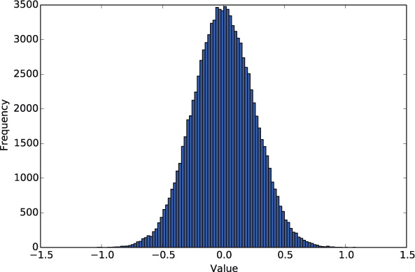
Figure 5.4 shows a histogramhistogram of 100,000 values returned by random.gauss(0, 0.25). Notice that the “bell curve” of frequencies is centered at the mean of 0.
The central limit theorem
Intuitively, the normal distribution is so common because phenomena that are the sums of many additive random factors tend to be normal. For example, a person’s height is the result of several different genes and the person’s health, so the distribution of heights in a population tends to be normal. To illustrate this phenomenon, let’s create a histogram of the sums of numbers generated by the random function. Below, the sumRandom function returns the sum of n random numbers in the interval [0, 1). The sumRandomHist function creates a list named samples that contains trials of these sums, and then plots a histogram of them.
import matplotlib.pyplot as pyplot
import random

def sumRandom(n):
    """Returns the sum of n pseudorandom numbers in [0,1).

     Parameter:
         n: the number of pseudorandom numbers to generate

     Return value: the sum of n pseudorandom numbers in [0,1)
     """

     sum = 0
     for index in range(n):
         sum = sum + random.random()
     return sum

def sumRandomHist(n, trials):
    """Displays a histogram of sums of n pseudorandom numbers.

     Parameters:
         n: the number of pseudorandom numbers in each sum
         trials: the number of sums to generate

     Return value: None
     """

     samples = [ ]
     for index in range(trials):
         samples.append(sumRandom(n))
     pyplot.hist(samples, 100)
     pyplot.show()
Reflection 5.16 Call sumRandomHist with 100,000 trials and values of n equal to 1, 2, 3, and 10. What do you notice?
When we call sumRandomHist with n = 1, we get the expected uniform distribution of values, shown in the upper left of Figure 5.5. However, for increasing values of n, we notice that the distribution of values very quickly begins to look like a normal distribution, as illustrated in the rest of Figure 5.5. In addition, the standard deviation of the distribution (intuitively, the width of the “bell”) appears to get smaller relative to the mean.
The mathematical name for this phenomenon is the central limit theorem. Intuitively, the central limit theorem implies that any large set of independent measurements of a process that is the cumulative result of many random factors will look like a normal distribution. Because a normal distribution is centered around a mean, this also implies that the average of all of the measurements will be close to the true mean.

Reflection 5.17 Think back to the experiment you ran to answer Reflection 5.9. The shape of the histogram should have resembled a normal distribution. Can you use the central limit theorem to explain why?
Exercises
5.3.1. A more realistic random walk has the movement in each step follow a normal distribution. In particular, in each step, we can change both x and y according to a normal distribution with mean 0. Because the values produced by this distribution will be both positive and negative, the particle can potentially move in any direction. To make the step sizes small, we need to use a small standard deviation, say 0.5:
x = x + random.gauss(0, 0.5)
y = y + random.gauss(0, 0.5)
Modify the randomWalk function so that it updates the position of the particle in this way instead. Then use the rwMonteCarlo and plotDistances functions to run a Monte Carlo simulation with your new randomWalk function. As we did earlier, call plotDistances(1000, 10000). How do your results differ from the original version?
5.3.2. Write a function
uniform(a, b)
that returns a number in the interval [a, b) using only the random.random function. (Do not use the random.uniform function.)
5.3.3. Suppose we want a pseudorandom integer between 0 and 7 (inclusive). How can we use the random.random() and int functions to get this result?
5.3.4. Write a function
randomRange(a, b)
that returns a pseudorandom integer in the interval [a . . b] using only the random.random function. (Do not use random.randrange or random.randint.)
5.3.5. Write a function
normalHist(mean, stdDev, trials)
that produces a histogram of trials values returned by the gauss function with the given mean and standard deviation. In other words, reproduce Figure 5.4. (This is very similar to the sumRandomHist function.)
5.3.6. Write a function
uniformHist(a, b, trials)
that produces a histogram of trials values in the range [a, b] returned by the uniform function. In other words, reproduce the top left histogram in Figure 5.5. (This is very similar to the sumRandomHist function.)
5.3.7. Write a function
plotChiSquared(k, trials)
that produces a histogram of trials values, each of which is the sum of k squares of values given by the random.gauss function with mean 0 and standard deviation 1. (This is very similar to the sumRandomHist function.) The resulting probability distribution is known as the chi-squared distribution (χ2 distribution) with k degrees of freedom.
5.4 BACK TO BOOLEANS
As we discussed at the beginning of the chapter, virtually every useful algorithm must be able to conditionally change course in response to input. This conditional behavior can be implemented with the same if statements that we worked with in Section 5.1. In this section, we will further develop your facility with these conditional statements, and the Boolean logic that drives them. (If your Boolean logic is rusty, you may want to review the concepts in Section 1.4 before continuing.)
In Section 5.1, we used simple if statements like
if r < 0.5:
    x = x + 1
else:
    x = x - 1
to control a random walk based on a random value of r. The outcome in this case is based upon the value of the Boolean expression r < 0.5. In Python, Boolean expressions evaluate to either the value True or the value False, which correspond to the binary values 1 and 0, respectively, that we worked with in Section 1.4. The values True and False can be printed, assigned to variable names, and manipulated just like numeric values. For example, try the following examples and make sure you understand each result.
>>> print(0 < 1)
True
>>> name = 'Kermit'
>>> print(name == 'Gonzo')
False
>>> result = 0 < 1
>>> result
True
>>> result and name == 'Kermit'
True
The “double equals” (==) operator tests for equality; it has nothing to do with assignment. The Python interpreter will remind you if you mistakenly use a single equals in an if statement. For example, try this:
>>> if r = 0:
    if r = 0:
         ^
SyntaxError: invalid syntax
However, the interpreter will not catch the error if you mistakenly use == in an assignment statement. For example, try this:
>>> r = 1
>>> r == r + 1   # increment r?
False
In a program, nothing will be printed as a result of the second statement, and r will not be incremented as expected. So be careful!
As we saw in Section 1.4, Boolean expressions can be combined with the Boolean operators (or logical operators) and, or, and not. As a reminder, Figure 5.6 contains the truth tables for the three Boolean operators, expressed in Python notation. In the tables, the variable names a and b represent arbitrary Boolean variables or expressions.
For example, suppose we wanted to determine whether a household has an annual income within some range, say $40,000 to $65,000:

>>> income    = 53000
>>> income    >= 40000 and income <= 65000
True
>>> income    = 12000
>>> income    >= 40000 and income <= 65000
False
When 53000 is assigned to income, the two Boolean expressions income >= 40000 and income <= 65000 are both True, so income >= 40000 and income <= 65000 is also True. However, when 12000 is assigned to income, income >= 40000 is False, while income <= 65000 is True, so income >= 40000 and income <= 65000 is now False. We can also incorporate this test into a function that simply returns the value of the condition:
>>> def middleClass(income):
        return (income >= 40000 and income <= 65000)
>>> middleClass(53000)
True
>>> middleClass(12000)
False
Reflection 5.18 What would happen if we changed and to or in the middleClass function? For what values of income would the function return False?
If we changed the middleClass function to be
def middleClass(income):
    return (income >= 40000 or income <= 65000)    # WRONG!
it would always return True! Consider the three possible cases:
If
incomeis between40000and65000(inclusive), it will returnTruebecause both parts of theorexpression areTrue.If
income < 40000, it will returnTruebecauseincome <= 65000isTrue.If
income > 65000, it will returnTruebecauseincome >= 40000isTrue.
Short circuit evaluation
The and and or operators exhibit a behavior known as short circuit evaluation that comes in handy in particular situations. Since both operands of an and expression must be true for the expression to be true, the Python interpreter does not bother to evaluate the second operand in an and expression if the first is false. Likewise, since only one operand of an or expression must be true for the expression to be true, the Python interpreter does not bother to evaluate the second operand in an or expression if the first is true.
For example, suppose we wanted to write a function to decide, in some for-profit company, whether the CEO’s compensation divided by the average employees’ is at most some “fair” ratio. A simple function that returns the result of this test looks like this:
def fair(employee, ceo, ratio):
    """Decide whether the ratio of CEO to employee pay is fair.

    Parameters:
        employee: average employee pay
        ceo: CEO pay
        ratio: the fair ratio

    Return: a Boolean indicating whether ceo / employee is fair
    """

    return (ceo / employee <= ratio)
Reflection 5.19 There is a problem with this function. What is it?
This function will not always work properly because, if the average employees’ compensation equals 0, the division operation will result in an error. Therefore, we have to test whether employee == 0 before attempting the division and, if so, return False (because not paying employees is obviously never fair). Otherwise, we want to return the result of the fairness test. The following function implements this algorithm.
def fair(employee, ceo, ratio):
    """ (docstring omitted) """

    if employee == 0:
        result = False
    else:
        result = (ceo / employee <= ratio)
    return result
However, with short circuit evaluation, we can simplify the whole function to:
def fair(employee, ceo, ratio):
    """ (docstring omitted) """

     return (employee != 0) and (ceo / employee <= ratio)
If employee is 0, then (employee != 0) is False, and the function returns False without evaluating (ceo / employee <= ratio). On the other hand, if (employee != 0) is true, then (ceo / employee <= ratio) is evaluated, and the return value depends on this outcome. Notice that this would not work if the and operator did not use short circuit evaluation because, if (employee != 0) were false and then (ceo / employee <= ratio) was evaluated, the division would result in a “divide by zero” error!
To illustrate the analogous mechanism with the or operator, suppose we wanted to write the function in the opposite way, instead returning True if the ratio is unfair. The first version of the function would look like this:
def unfair(employee, ceo, ratio):
    """Decide whether the ratio of CEO to employee pay is unfair.

     Parameters:
         employee: average employee pay
         ceo: CEO pay
         ratio: the fair ratio

     Return: a Boolean indicating whether ceo / employee is not fair
     """

     if employee == 0:
         result = True
     else:
         result = (ceo / employee > ratio)
     return result
However, taking advantage of short circuit evaluation with the or operator, we can simplify the whole function to:
def unfair(employee, ceo, ratio):
    """ (docstring omitted) """

     return (employee == 0) or (ceo / employee > ratio)
In this case, if (employee == 0) is True, the whole expression returns True without evaluating the division test, thus avoiding an error. On the other hand, if (employee == 0) is False, the division test is evaluated, and the final result is equal to the outcome of this test.
Complex expressions
Some situations require Boolean expressions that are more complex than what we have seen thus far. To illustrate, let’s consider how to test whether a particle in a random walk at position (x, y) is in one of the four corners of the screen, as depicted by the shaded regions below.

There are (at least) two ways we can write a Boolean expression to test this condition. One way is to test whether the particle is in each corner individually.
For the point to be corner 1,
x > d and y > dmust beTrue;for the point to be corner 2,
x < -d and y > dmust beTrue;for the point to be corner 3,
x < -d and y < -dmust beTrue; orfor the point to be corner 4,
x > d and y < -dmust beTrue.
Since any one of these can be True for our condition to be True, the final test, in the form of a function, looks like the following. (The “backslash” () character below is the line continuation character. It indicates that the line that it ends is continued on the next line. This is sometimes handy for splitting very long lines of code.)
>>> def corners(x, y, d):
        return x > d and y > d or x < -d and y > d or
               x < -d and y < -d or x > d and y < -d
>>> corners(11, -11, 10)
True
>>> corners(11, 0, 10)
False
Although our logic is correct, this expression is only correct if the Python interpreter evaluates the and operator before it evaluates the or operator. Otherwise, if the or operator is evaluated first, then the first expression evaluated will be y > d or x < -d, shown in red below, which is not what we intended.

Table 5.2 Operator precedence, listed from highest to lowest. This is an expanded version of Table 2.1.
x > d and y > d or x < -d and y > d or x < -d and y < -d or x > d and y < -d
Therefore, understanding the order in which operators are evaluated, known as operator precedence, becomes important for more complex conditions such as this. In this case, the expression is correct because and has precedence over or, as illustrated in Table 5.2. Also notice from Table 5.2 that the comparison operators have precedence over the Boolean operators, which is also necessary for our expression to be correct. If in doubt, you can use parentheses to explicitly specify the intended order. Parentheses would be warranted here in any case, to make the expression more understandable:
>>> def corners(x, y, d):
        return (x > d and y > d) or (x < -d and y > d) or
               (x < -d and y < -d) or (x > d and y < -d)
Now let’s consider an alternative way to think about the corner condition: for a point to be in one of the corners, it must be true that x must either exceed d or be less than -d and y must either exceed d or be less than -d. The equivalent Boolean expression is enclosed in the following function.
>>> def corners2(x, y, d):
        return x > d or x < -d and y > d or y < -d
>>> corners2(11, -11, 10)
True
>>> corners2(11, 0, 10)
True
Reflection 5.20 The second call to corners2 gives an incorrect result. Do you see the problem? (You might want to draw a picture.)
Due to the operator precedence order, this is a situation where parentheses are required. Without parentheses, the and expression in red below is evaluated first, which is not our intention.
x > d or x < -d and y > d or y < -d
So the correct implementation is
>>> def corners2(x, y, d):
        return (x > d or x < -d) and (y > d or y < -d)
>>> corners2(11, -11, 10)
True
>>> corners2(11, 0, 10)
False
*Using truth tables
Reflection 5.21 How can we confirm that this expression is really correct?
To confirm that any Boolean expression is correct, we must create a truth table for it, and then confirm that every case matches what we intended. In this expression, there are four separate Boolean “inputs,” one for each expression containing a comparison operator. In the truth table, we will represent each of these with a letter to save space:
x > dwill be represented by p,x < -dwill be represented by q,y > dwill be represented by r, andy < -dwill be represented by s.
So the final expression we are evaluating is (p or q) and (r or s).
In the truth table below, the first four columns represent our four inputs. With four inputs, we need 24 = 16 rows, one for each possible assignment of truth values to the inputs. There is a trick to quickly writing down all the truth value combinations; see if you can spot it in the first four columns. (We are using T and F as abbreviations for True and False. The extra horizontal lines are simply to improve readability.)
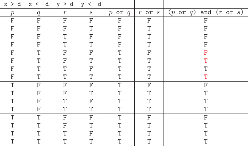
To fill in the fifth column, we only need to look at the first and second columns. Since this is an or expression, for each row in the fifth column, we enter a T if there is at least one T among the first and second columns of that row, or a F otherwise. Similarly, to fill in the sixth column, we only look at the third and fourth column. To fill in the last column, we look at the two previous columns, filling in a T in each row in which the fifth and sixth columns are both T, or a F otherwise.
To confirm that our expression is correct, we need to confirm that the truth value in each row of the last column is correct with respect to that row’s input values. For example, let’s look at the fifth, sixth, and eighth rows of the truth table (in red).
In the fifth row, the last column indicates that the expression is False. Therefore, it should be the case that a point described by the truth values in the first four columns of that row is not in one of the four corners. Those truth values say that x > d is false, x < -d is true, y > d is false, and y < -d is false; in other words, x is less than -d and y is between -d and d. A point within these bounds is not in any of the corners, so that row is correct.
Now let’s look at the sixth row, where the final expression is true. The first columns of that row indicate that x > d is false, x < -d is true, y > d is false, and y < -d is true; in other words, both x and y are less than -d. A point within these bounds is in the bottom left corner, so that row is also correct.
The eighth row is curious because it states that both y > d and y < -d are true. But this is, of course, impossible. Because of this, we say that the implied statement is vacuously true. In practice, we cannot have such a point, so that row is entirely irrelevant. There are seven such rows in the table, leaving only four other rows that are true, matching the four corners.
Many happy returns
We often come across situations in which we want an algorithm (i.e., a function) to return different values depending on the outcome of a condition. The simplest example is finding the maximum of two numbers a and b. If a is at least as large as b, we want to return a; otherwise, b must be larger, so we return b.
def max(a, b):
    """Returns the maximum of a and b.

    Parameters:
        a, b: two numbers

    Return value: the maximum value
    """

    if a >= b:
        result = a
    else:
        result = b
    return result
We can simplify this function a bit by returning the appropriate value right in the if/else statement:
def max(a, b):
    """ (docstring omitted)"""

    if a >= b:
        return a
    else:
        return b
It may look strange at first to see two return statements in one function, but it all makes perfect sense. Recall from Section 3.5 that return both ends the function and assigns the function’s return value. So this means that at most one return statement can ever be executed in a function. In this case, if a >= b is true, the function ends and returns the value of a. Otherwise, the function executes the else clause, which returns the value of b.
The fact that the function ends if a >= b is true means that we can simplify it even further: if execution continues past the if part of the if/else, it must be the case that a >= b is false. So the else is extraneous; the function can be simplified to:
def max(a, b):
    """ (docstring omitted)"""

     if a >= b:
         return a
     return b
This same principle can be applied to situations with more than two cases. Suppose we wrote a function to convert a percentage grade to a grade point (i.e., GPA) on a 0–4 scale. A natural implementation of this might look like the following:
def assignGP(score):
    """Returns the grade point equivalent of score.

     Parameter:
         score: a score between 0 and 100

     Return value: the equivalent grade point value
     """

     if score >= 90:
         return 4
     elif score >= 80:
         return 3
     elif score >= 70:
         return 2
     elif score >= 60:
         return 1
     else:
         return 0
Reflection 5.22 Why do we not need to check upper bounds on the scores in each case? In other words, why does the second condition not need to be score >= 80 and score < 90?
Suppose score was 92. In this case, the first condition is true, so the function returns the value 4 and ends. Execution never proceeds past the statement return 4. For this reason, the “el” in the next elif is extraneous. In other words, because execution would never have made it there if the previous condition was true, there is no need to tell the interpreter to skip testing this condition if the previous condition was true.
Now suppose score was 82. In this case, the first condition would be false, so we continue on to the first elif condition. Because we got to this point, we already know that score < 90 (hence the omission of that check). The first elif condition is true, so we immediately return the value 3. Since the function has now completed, there is no need for the “el” in the second elif either. In other words, because execution would never have made it to the second elif if either of the previous conditions were true, there is no need to skip testing this condition if a previous condition was true. In fact, we can remove the “el”s from all of the elifs, and the final else, with no loss in efficiency at all.
def assignGP(score):
    """ (docstring omitted) """

      if score >= 90:
          return 4
      if score >= 80:
          return 3
      if score >= 70:
          return 2
      if score >= 60:
          return 1
      return 0
Some programmers find it clearer to leave the elif statements in, and that is fine too. We will do it both ways in the coming chapters. But, as you begin to see more algorithms, you will probably see code like this, and so it is important to understand why it is correct.
Exercises
5.4.1. Write a function
password()
that asks for a username and a password. It should return True if the username is entered as alan.turing and the password is entered as notTouring, and return False otherwise.
5.4.2. Suppose that in a game that you are making, the player wins if her score is at least 100. Write a function
hasWon(score)
that returns True if she has won, and False otherwise.
5.4.3. Suppose you have designed a sensor that people can wear to monitor their health. One task of this sensor will be to monitor body temperature: if it falls outside the range 97.9° F to 99.3° F, the person may be getting sick. Write a function
monitor(temperature)
that takes a temperature (in Fahrenheit) as a parameter, and returns True if temperature falls in the healthy range and False otherwise.
5.4.4. Write a function
winner(score1, score2)
that returns 1 or 2, indicating whether the winner of a game is Player 1 or Player 2. The higher score wins and you can assume that there are no ties.
5.4.5. Repeat the previous exercise, but now assume that ties are possible. Return 0 to indicate a tie.
5.4.6. Your firm is looking to buy computers from a distributor for $1500 per machine. The distributor will give you a 5% discount if you purchase more than 20 computers. Write a function
cost(quantity)
that takes as a parameter the quantity of computers you wish to buy, and returns the cost of buying them from this distributor.
5.4.7. Repeat the previous exercise, but now add three additional parameters: the cost per machine, the number of computers necessary to get a discount, and the discount.
5.4.8. The speeding ticket fine in a nearby town is $50 plus $5 for each mph over the posted speed limit. In addition, there is an extra penalty of $200 for all speeds above 90 mph. Write a function
fine(speedLimit, clockedSpeed)
that returns the fine amount (or 0 if clockedSpeed ≤ speedLimit).
5.4.9. Write a function
gradeRemark()
that prompts for a grade, and then returns the corresponding remark (as a string) from the table below:
| Grade | Remark |
| 96-100 | Outstanding |
| 90-95 | Exceeds expectations |
| 80-89 | Acceptable |
| 1-79 | Trollish |
5.4.10. Write a function that takes two integer values as parameters and returns their sum if they are not equal and their product if they are.
5.4.11. Write a function
amIRich(amount, rate, years)
that accumulates interest on amount dollars at an annual rate of rate percent for a number of years. If your final investment is at least double your original amount, return True; otherwise, return False.
5.4.12. Write a function
max3(a, b, c)
the returns the maximum value of the parameters a, b, and c. Be sure to test it with many different numbers, including some that are equal.
5.4.13. Write a function
shipping(amount)
that returns the shipping charge for an online retailer based on a purchase of amount dollars. The company charges a flat rate of $6.95 for purchases up to $100, plus 5% of the amount over $100.
5.4.14. Starting with two positive integers a and b, consider the sequence in which the next number is the digit in the ones place of the sum of the previous two numbers. For example, if a = 1 and b = 1, the sequence is
1, 1, 2, 3, 5, 8, 3, 1, 4, 5, 9, 4, 3, 7, 0, ...
Write a function
mystery(a, b)
that returns the length of the sequence when the last two numbers repeat the values of a and b for the first time. (When a = 1 and b = 1, the function should return 62.)
5.4.15. The Chinese zodiac relates each year to an animal in a twelve-year cycle. The animals for the most recent years are given below.

Write a function
zodiac(year)
that takes as a parameter a four-digit year (this could be any year in the past or future) and returns the corresponding animal as a string.
5.4.16. A year is a leap year if it is divisible by four, unless it is a century year in which case it must be divisible by 400. For example, 2012 and 1600 are leap years, but 2011 and 1800 are not. Write a function
leap(year)
that returns a Boolean value indicating whether the year is a leap year.
5.4.17. Write a function
even(number)
that returns True if number is even, and False otherwise.
5.4.18. Write a function
between(number, low, high)
that returns True if number is in the interval [low, high] (between (or equal to) low and high), and False otherwise.
5.4.19. Write a function
justone(a, b)
that returns True if exactly one (but not both) of the numbers a or b is 10, and False otherwise.
5.4.20. Write a function
roll()
that simulates rolling two of the loaded dice implemented in Exercise 5.1.3 (by calling the function loaded), and returns True if the sum of the dice is 7 or 11, or False otherwise.
5.4.21. The following function returns a Boolean value indicating whether an integer number is a perfect square. Rewrite the function in one line, taking advantage of the short-circuit evaluation of and expressions.
def perfectSquare(number):
    if number < 0:
        return False
    else:
        return math.sqrt(number) == int(math.sqrt(number))
5.4.22. Consider the rwMonteCarlo function on Page 193. What will the function return if trials equals 0? What if trials is negative? Propose a way to deal with these issues by adding statements to the function.
5.4.23. Write a Boolean expression that is True if and only if the point (x, y) resides in the shaded box below (including its boundary).

5.4.24. Use a truth table to show that the Boolean expressions
(x > d and y > d) or (x < -d and y > d)
and
(y > d) and (x > d or x < -d)
are equivalent.
drawRow(tortoise, row)
that uses turtle graphics to draw one row of an 8 × 8 red/black checkerboard. If the value of row is even, the row should start with a red square; otherwise, it should start with a black square. You may want to use the drawSquare function you wrote in Exercise 3.3.5. Your function should only need one for loop and only need to draw one square in each iteration.
5.4.26. Write a function
checkerBoard(tortoise)
that draws an 8 × 8 red/black checkerboard, using the function you wrote in Exercise 5.4.25.
5.5 A GUESSING GAME
In this section, we will practice a bit more writing algorithms that contain complex conditional constructs and while loops by designing an algorithm that lets us play the classic “I’m thinking of a number” game with the computer. The computer (really the PRNG) will “think” of a number between 1 and 100, and we will try to guess it. Here is a function to play the game:
import random

def guessingGame(maxGuesses):
    """Plays a guessing game. The human player tries to guess
       the computer's number from 1 to 100.

    Parameter:
        maxGuesses: the maximum number of guesses allowed

    Return value: None
    """

    secretNumber = random.randrange(1, 101)
    for guesses in range(maxGuesses):
        myGuess = input('Please guess my number: ')
        myGuess = int(myGuess)

         if myGuess == secretNumber:    # win
             print('You got it!')
         else:                          # try again
             print('Nope. Try again.')
The randrange function returns a random integer that is at least the value of its first argument, but less than its second argument (similar to the way the range function interprets its arguments). After the function chooses a random integer between 1 and 100, it enters a for loop that will allow us to guess up to maxGuesses times. The function prompts us for our guess with the input function, and then assigns the response to myGuess as a string. Because we want to interpret the response as an integer, we use the int function to convert the string. Once it has myGuess, the function uses the if/else statement to tell us whether we have guessed correctly. After this, the loop will give us another guess, until we have used them all up.
Reflection 5.23 Try playing the game by calling guessingGame(20). Does it work? Is there anything we still need to work on?
You may have noticed three issues:
After we guess correctly, unless we have used up all of our guesses, the loop iterates again and gives us another guess. Instead, we want the function to end at this point.
It would be much friendlier for the game to tell us whether an incorrect guess is too high or too low.
If we do not guess correctly in at most
maxGuessesguesses, the last thing we see is'Nope. Try again.'before the function ends. But there is no opportunity to try again; instead, it should tell us that we have lost.
We will address these issues in order.
1. Ending the game if we win
Our current for loop, like all for loops, iterates a prescribed number of times. Instead, we want the loop to only iterate for as long as we need another guess. So this is another instance that calls for a while loop. Recall that a while loop iterates while some Boolean condition is true. In this case, we need the loop to iterate while we have not guessed the secret number, in other words, while myGuess != secretNumber. But we also need to stop when we have used up all of our guesses, counted in our current function by the index variable guesses. So we also want our while loop to iterate while guesses < maxGuesses. Since both of these conditions must be true for us to keep iterating, our desired while loop condition is:
while (myGuess != secretNumber) and (guesses < maxGuesses):
Because we are replacing our for loop with this while loop, we will now need to manage the index variable manually. We do this by initializing guesses = 0 before the loop and incrementing guesses in the body of the loop. Here is the function with these changes:
def guessingGame(maxGuesses):
    """ (docstring omitted) """

    secretNumber = random.randrange(1, 101)
    myGuess = 0
    guesses = 0
    while (myGuess != secretNumber) and (guesses < maxGuesses):
        myGuess = input('Please guess my number: ')
        myGuess = int(myGuess)
        guesses = guesses + 1          # increment # of guesses
        if myGuess == secretNumber:    # win
            print('You got it!')
        else:                          # try again
            print('Nope. Try again.')
Reflection 5.24 Notice that we have also included myGuess = 0 before the loop. Why do we bother to assign a value to myGuess before the loop? Is there anything special about the value 0? (Hint: try commenting it out.)
If we comment out myGuess = 0, we will see the following error on the line containing the while loop:
UnboundLocalError: local variable 'myGuess' referenced before assignment
This error means that we have referred to an unknown variable named myGuess. The name is unknown to the Python interpreter because we had not defined it before it was first referenced in the while loop condition. Therefore, we need to initialize myGuess before the while loop, so that the condition makes sense the first time it is tested. To make sure the loop iterates at least once, we need to initialize myGuess to a value that cannot be the secret number. Since the secret number will be at least 1, 0 works for this purpose. This logic can be generalized as one of two rules to always keep in mind when designing an algorithm with a while loop:
Initialize the condition before the loop. Always make sure that the condition makes sense and will behave in the intended way the first time it is tested.
In each iteration of the loop, work toward the condition eventually becoming false. Not doing so will result in an infinite loop.
To ensure that our condition will eventually become false, we need to understand when this happens. For the and expression in the while loop to become false, either (myGuess != secretNumber) must be false or (guesses < maxGuesses) must be false.
Reflection 5.25 How do the statements in the body of the loop ensure that eventually (myGuess != secretNumber) or (guesses < maxGuesses) will be false?
Prompting for a new guess creates the opportunity for the first part to become false, while incrementing guesses ensures that the second part will eventually become false. Therefore, we cannot have an infinite loop.
This reasoning is enshrined in the first of De Morgan’s laws, named after 19th century British mathematician Augustus De Morgan. De Morgan’s two laws are:
not (a and b) = not a or not b
not (a or b) = not a and not b
You may recognize these from Exercises 1.4.10 and 1.4.11. The first law says that a and b is false if either a is false or b is false. The second law says that a or b is false if both a is false and b is false. Applied to our case, the first law tells us that the negation of our while loop condition is
(myGuess == secretNumber) or (guesses >= maxGuesses)
This is just a more formal way of deriving what we already concluded.
2. Friendly hints
Inside the loop, we currently handle two cases: (1) we win, and (2) we do not win but get another guess. To be friendlier, we should split the second case into two: (2a) our guess was too low, and (2b) our guess was too high. We can accomplish this by replacing the not-so-friendly print('Nope. Try again.') with another if/else that decides between the two new subcases:
if myGuess == secretNumber:                   # win
    print('You got it!')
else:                                         # try again
    if myGuess < secretNumber:                # too low
        print('Too low. Try again.')
    else:                                     # too high
        print('Too high. Try again.')
Now, if myGuess == secretNumber is false, we execute the first else clause, the body of which is the new if/else construct. If myGuess < secretNumber is true, we print that the number is too low; otherwise, we print that the number is too high.
Reflection 5.26 Do you see a way in which the conditional construct above can be simplified?
The conditional construct above is really just equivalent to a decision between three disjoint possibilities: (a) the guess is equal to the secret number, (b) the guess is less than the secret number, or (c) the guess is greater than the secret number. In other words, it is equivalent to:
if myGuess == secretNumber:            # win
    print('You got it!')
elif myGuess < secretNumber:           # too low
    print('Too low. Try again.')
else:                                  # too high
    print('Too high. Try again.')
3. Printing a proper win/lose message
Now inside the loop, we currently handle three cases: (a) we win, and (b) our guess is too low and we get another guess, and (c) our guess is too high and we get another guess. But we are missing the case in which we run out of guesses. In this situation, we want to print something like 'Too bad. You lose.' instead of one of the “try again” messages.
Reflection 5.27 How can we augment the if/elif/else statement so that it correctly handles all four cases?
In the game, if we incorrectly use our last guess, then two things must be true just before the if condition is tested: first, myGuess is not equal to secretNumber and, second, guesses is equal to maxGuesses. So we can incorporate this condition into the if/elif/else:
if (myGuess != secretNumber) and (guesses == maxGuesses): # lose
    print('Too bad. You lose.')
elif myGuess == secretNumber:       # win
    print('You got it!')
elif myGuess < secretNumber:        # too low
    print('Too low. Try again.')
else:                               # too high
    print('Too high. Try again.')
Notice that we have made the previous first if condition into an elif statement because we only want one of the four messages to be printed. However, here is an alternative structure that is more elegant:
if myGuess == secretNumber:            # win
    print('You got it!')
elif guesses == maxGuesses:            # lose
    print('Too bad. You lose.')
elif myGuess < secretNumber:           # too low
    print('Too low. Try again.')
else:                                  # too high
    print('Too high. Try again.')
By placing the new condition second, we can leverage the fact that, if we get to the first elif, we already know that myGuess != secretNumber. Therefore, we do not need to include it explicitly.
There is a third way to handle this situation that is perhaps even more elegant. Notice that both of the first two conditions are going to happen at most once, and at the end of the program. So it might make more sense to put them after the loop. Doing so also exhibits a nice parallel between these two events and the two parts of the while loop condition. As we discussed earlier, the negation of the while loop condition is
(myGuess == secretNumber) or (guesses >= maxGuesses)
So when the loop ends, at least one of these two things is true. Notice that these two events are exactly the events that define a win or a loss: if the first part is true, then we won; if the second part is true, we lost. So we can move the win/loss statements after the loop, and decide which to print based on which part of the while loop condition became false:
if myGuess == secretNumber:            # win
    print('You got it!')
else:                                  # lose
    print('Too bad. You lose.')
In the body of the loop, with these two cases gone, we will now need to check if we still get another guess (mirroring the while loop condition) before we print one of the “try again” messages:
if (myGuess != secretNumber) and (guesses < maxGuesses):
    if myGuess < secretNumber:          # too low
        print('Too low. Try again.')
    else:                               # too high
        print('Too high. Try again.')
Reflection 5.28 Why is it not correct to combine the two if statements above into a single statement like the following?
if (myGuess != secretNumber) and (guesses < maxGuesses)
                             and (myGuess < secretNumber):
    print('Too low. Try again.')
else:
    print('Too high. Try again.')
Hint: what does the function print when guesses < maxGuesses is false and myGuess < secretNumber is true?
These changes are incorporated into the final game that is shown below.
import random

def guessingGame(maxGuesses):
    """ (docstring omitted) """

      secretNumber = random.randrange(1, 101)
      myGuess = 0
      guesses = 0
      while (myGuess != secretNumber) and (guesses < maxGuesses):
          myGuess = input('Please guess my number: ')
          myGuess = int(myGuess)
          guesses = guesses + 1         # increment # of guesses used

         if (myGuess != secretNumber) and (guesses < maxGuesses):
             if myGuess < secretNumber:          # guess is too low
                 print('Too low. Try again.')    #   give a hint
             else:                               # guess is too high
                 print('Too high. Try again.')   #     give a hint

      if myGuess == secretNumber:      # win
          print('You got it!')
      else:                            # lose
          print('Too bad. You lose.')

def main():
    guessingGame(10)

main()
As you play the game, think about what the best strategy is. How many guesses do different strategies require? Exercise 5.5.7 asks you to write a Monte Carlo simulation to compare three different strategies for playing the game.
Exercises
5.5.1. Write a function
ABC()
that prompts for a choice of A, B, or C and uses a while loop to keep prompting until it receives the string 'A', 'B', or 'C'.
5.5.2. Write a function
numberPlease()
that prompts for an integer between 1 and 100 (inclusive) and uses a while loop to keep prompting until it receives a number within this range.
5.5.3. Write a function
differentNumbers()
that prompts for two different numbers. The function should use a while loop to keep prompting for a pair of numbers until the two numbers are different.
5.5.4. Write a function
rockPaperScissorsLizardSpock(player1, player2)
that decides who wins in a game of rock-paper-scissors-lizard-Spock1. Each of player1 and player2 is a string with value 'rock', 'paper', 'scissors', 'lizard', or 'Spock'. The function should return the value 1 if player 1 wins, -1 if player 2 wins, or 0 if they tie. Test your function by playing the game with the following main program:
def main():
    player1 = input('Player1: ')
    player2 = input('Player2: ')

     outcome = rockPaperScissorsLizardSpock(player1, player2)

     if outcome == 1:
         print('Player 1 wins!')
     elif outcome == -1:
         print('Player 2 wins!')
     else:
         print('Player 1 and player 2 tied.')
5.5.5. Write a function
yearsUntilDoubled(amount, rate)
that returns the number of years until amount is doubled when it earns the given rate of interest, compounded annually. Use a while loop.
5.5.6. The hailstone numbers are a sequence of numbers generated by the following simple algorithm. First, choose any positive integer. Then, repeatedly follow this rule: if the current number is even, divide it by two; otherwise, multiply it by three and add one. For example, suppose we choose the initial integer to be 3. Then this algorithm produces the following sequence:
3, 10, 5, 16, 8, 4, 2, 1, 4, 2, 1, 4, 2, 1 ...
For every initial integer ever tried, the sequence always reaches one and then repeats the sequence 4, 2, 1 forever after. Interestingly, however, no one has ever proven that this pattern holds for every integer!
Write a function
hailstone(start)
that prints the hailstone number sequence starting from the parameter start, until the value reaches one. Your function should return the number of integers in your sequence. For example, if n were 3, the function should return 8. (Use a while loop.)
5.5.7. In this exercise, we will design a Monte Carlo simulation to compare the effectiveness of three strategies for playing the guessing game. Each of these strategies will be incorporated into the guessing game function we designed in this chapter, but instead of checking whether the player wins or loses, the function will continue until the number is guessed, and then return the number of guesses used. We will also make the maximum possible secret number a parameter, so that we can compare the results for different ranges of secret numbers.
The first strategy is to just make a random guess each time, ignoring any previous guesses:
def guessingGame1(maxNumber):
    """Play the guessing game by making random guesses."""

     secretNumber = random.randrange(1, maxNumber + 1)
     myGuess = 0
     guesses = 0
     while (myGuess != secretNumber):
         myGuess = random.randrange(1, maxNumber + 1)
         guesses = guesses + 1

     return guesses
The second strategy is to incrementally try every possible guess from 1 to 100, thereby avoiding any duplicates:
def guessingGame2(maxNumber):
    """Play the guessing game by making incremental guesses."""

     secretNumber = random.randrange(1, maxNumber + 1)
     myGuess = 0
     guesses = 0
     while (myGuess != secretNumber):
         myGuess = myGuess + 1
         guesses = guesses + 1

     return guesses
Finally, the third strategy uses the outcomes of previous guesses to narrow in on the secret number:
def guessingGame3(maxNumber):
    """Play the guessing game intelligently by narrowing in
       on the secret number."""

     secretNumber = random.randrange(1, maxNumber + 1)
     myGuess = 0
     low = 1
     high = maxNumber
     guesses = 0
     while (myGuess != secretNumber):
         myGuess = (low + high) // 2
         guesses = guesses + 1

          if myGuess < secretNumber:
              low = myGuess + 1
          elif myGuess > secretNumber:
              high = myGuess - 1

     return guesses
Write a Monte Carlo simulation to compare the expected (i.e., average) behavior of these three strategies. Use a sufficiently high number of trials to get consistent results. Similarly to what we did in Section 5.1, run your simulation for a range of maximum secret numbers, specifically 5, 10, 15, ..., 100, and plot the average number of guesses required by each strategy for each maximum secret number. (The x-axis of your plot will be the maximum secret number and the y-axis will be the average number of guesses.) Explain the results. In general, how many guesses on average do you think each strategy requires to guess a secret number between 1 and n?
5.6 SUMMARY
In previous chapters, we designed deterministic algorithms that did the same thing every time we executed them, if we gave them the same inputs (i.e., arguments). Giving those algorithms different arguments, of course, could change their behavior, whether it be drawing a different size shape, modeling a different population, or experimenting with a different investment scenario. In this chapter, we started to investigate a new class of algorithms that can change their behavior “on the fly,” so to speak. These algorithms all make choices using Boolean logic, the same Boolean logic on which computers are fundamentally based. By combining comparison operators and Boolean operators, we can characterize just about any decision. By incorporating these Boolean expressions into conditional statements (if/elif/else) and conditional loops (while), we vastly increase the diversity of algorithms that we can design. These are fundamental techniques that we will continue to use and develop over the next several chapters, as we start to work with textual and numerical data that we read from files and download from the web.
5.7 FURTHER DISCOVERY
This chapter’s epigraph is a famous “Yogiism,” from Hall of Fame catcher, coach, and manager Yogi Berra [6].
If you would like to learn more about Robert Brown’s experiments, and the history and science behind them, visit the following web site, titled “What Brown Saw and You Can Too.”
http://physerver.hamilton.edu/Research/Brownian/index.html
The Drunkard’s Walk by Leonard Mlodinow [34] is a very accessible book about how randomness and chance affect our lives. For more information about generating random numbers, and the differences between PRNGs and true random number generators, visit
https://www.random.org/randomness/.
The Park-Miller random number generator is due to Keith Miller and the late Steve Park [37].
The Roper Center for Public Opinion Research, at the University of Connecticut, maintains some helpful educational resources about random sampling and errors in the context of public opinion polling at
http://www.ropercenter.uconn.edu/education.html.
5.8 PROJECTS
Project 5.1 The magic of polling
According to the latest poll, the president’s job approval rating is at 45%, with a margin of error of ±3%, based on interviews with approximately 1,500 adults over the weekend.
We see news headlines like this all the time. But how can a poll of 1,500 randomly chosen people claim to represent the opinions of millions in the general population? How can the pollsters be so certain of the margin of error? In this project, we will investigate how well random sampling can really estimate the characteristics of a larger population. We will assume that we know the true percentage of the overall population with some characteristic or belief, and then investigate how accurate a much smaller poll is likely to get.
Suppose we know that 30% of the national population agrees with the statement, “Animals should be afforded the same rights as human beings.” Intuitively, this means that, if we randomly sample ten individuals from this population, we should, on average, find that three of them agree with the statement and seven do not. But does it follow that every poll of ten randomly chosen people will mirror the percentage of the larger population? Unlike a Monte Carlo simulation, a poll is taken just once (or maybe twice) at any particular point in time. To have confidence in the poll results, we need some assurance that the results would not be drastically different if the poll had queried a different group of randomly chosen individuals. For example, suppose you polled ten people and found that two agreed with the statement, then polled ten more people and found that seven agreed, and then polled ten more people and found that all ten agreed. What would you conclude? There is too much variation for this poll to be credible. But what if we polled more than ten people? Does the variation, and hence the trustworthiness, improve?
In this project, you will write a program to investigate questions such as these and determine empirically how large a sample needs to be to reliably represent the sentiments of a large population.
1. Simulate a poll
In conducting this poll, the pollster asks each randomly selected individual whether he or she agrees with the statement. We know that 30% of the population does, so there is a 30% chance that each individual answers “yes.” To simulate this polling process, we can iterate over the number of individuals being polled and count them as a “yes” with probability 0.3. The final count at the end of the loop, divided by the number of polled individuals, gives us the poll result. Implement this simulation by writing a function
poll(percentage, pollSize)
that simulates the polling of pollSize individuals from a large population in which the given percentage (between 0 and 100) will respond “yes.” The function should return the percentage (between 0 and 100) of the poll that actually responded “yes.” Remember that the result will be different every time the function is called. Test your function with a variety of poll sizes.
2. Find the polling extremes
To investigate how much variation there can be in a poll of a particular size, write a function
pollExtremes(percentage, pollSize, trials)
that builds a list of trials poll results by calling poll(percentage, pollSize) trials times. The function should return the minimum and maximum percentages in this list. For example, if five trials give the percentages [28, 35, 31, 24, 31], the function should return the minimum 24 and maximum 35. If the list of poll results is named pollResults, you can return these two values with
return min(pollResults), max(pollResults)
Test your function with a variety of poll sizes and numbers of trials.
3. What is a sufficient poll size?
Next, we want to use your previous functions to investigate how increasing poll sizes affect the variation of the poll results. Intuitively, the more people you poll, the more accurate the results should be. Write a function
plotResults(percentage, minPollSize, maxPollSize, step, trials)
that plots the minimum and maximum percentages returned by calling the function pollExtremes(percentage, pollSize, trials) for values of pollSize ranging from minPollSize to maxPollSize, in increments of step. For each poll size, call your pollExtremes function with
low, high = pollExtremes(percentage, pollSize, trials)
and then append the values of low and high each to its own list for the plot. Your function should return the margin of error for the largest poll, defined to be (high - low) / 2. The poll size should be on the x-axis of your plot and the percentage should be on the y-axis. Be sure to label both axes.
Question 5.1.1 Assuming that you want to balance a low margin of error with the labor involved in polling more people, what is a reasonable poll size? What margin of error does this poll size give?
Write a main function (if you have not already) that calls your plotResults function to investigate an answer to this question. You might start by calling it with plotResults(30, 10, 1000, 10, 100).
4. Does the error depend on the actual percentage?
To investigate this question, write another function
plotErrors(pollSize, minPercentage, maxPercentage, step, trials)
that plots the margin of error in a poll of pollSize individuals, for actual percentages ranging from minPercentage to maxPercentage, in increments of step. To find the margin of error for each poll, call the pollExtremes function as above, and compute (high - low) / 2. In your plot, the percentage should be on the x-axis and the margin of error should be on the y-axis. Be sure to label both axes.
Question 5.1.2 Does your answer to the previous part change if the actual percentage of the population is very low or very high?
You might start to investigate this question by calling the function with plotErrors(1500, 10, 80, 1, 100).
Project 5.2 Escape!
In some scenarios, movement of the “particle” in a random walk is restricted to a bounded region. But what if there is a small opening through which the particle might escape or disappear? How many steps on average does it take the particle to randomly come across this opening and escape? This model, which has become known as the narrow escape problem, could represent a forager running across a predator on the edge its territory, an animal finding an unsecured gate in a quarantined area, a molecule finding its way through a pore in the cell membrane, or air molecules in a hot room escaping through an open door.
1. Simulate the narrow escape
Write a function
escape(openingDegrees, tortoise, draw)
that simulates the narrow escape problem in a circle with radius 1 and an opening of openingDegrees degrees. In the circle, the opening will be between 360 – openingDegrees and 360 degrees, as illustrated below.

The particle should follow a normally distributed random walk, as described in Exercise 5.3.1. The standard deviation of the normal distribution needs to be quite small for the particle to be able to find small openings. A value of π/128 is suggested in [7]. Since we are interested in the number of steps taken by the particle (instead of the distance traveled, as before), the number of steps will need to be incremented in each iteration of the loop. When the particle hits a wall, it should “bounce” back to its previous position. Since the particle is moving within a circle, we can tell if it hits a wall by comparing its distance from the origin to the radius of the circle. If the particle moves out to the distance of the wall, but is within the angle of the opening, the loop should end, signaling the particle’s escape.
Finding the current angle of the particle with respect to the origin requires some trigonometry. Since we know the x and y coordinates of the particle, the angle can be found by computing the arctangent of y/x: tan−1(y/x). However, this will cause a problem with x = 0, so we need to check for that possibility and fudge the value of x a bit. Also, the Python arctangent (tan−1) function, math.atan, always returns an angle between −π/2 and π/2 radians (between −90 and 90 degrees), so the result needs to be adjusted to be between 0 and 360 degrees. The following function handles this for you.
def angle(x, y):
    if x == 0:       # avoid dividing by zero
        x = 0.001
    angle = math.degrees(math.atan(y / x))
    if angle < 0:
        if y < 0:
            angle = angle + 360   # quadrant IV
        else:
            angle = angle + 180   # quadrant II
    elif y < 0:
        angle = angle + 180       # quadrant III
    return angle
Below you will find a “skeleton” of the escape function with the loop and drawing code already written. Drawing the partial circle is handled by the function setupWalls below. Notice that the function uses a while loop with a Boolean flag variable named escaped controlling the iteration. The value of escaped is initially False, and your algorithm should set it to True when the particle escapes. Most, but not all, of the remaining code is needed in the while loop.
def escape(openingDegrees, tortoise, draw):
    x = y = 0                     # initialize (x, y) = (0, 0)
    radius = 1                    # moving in unit radius circle
    stepLength = math.pi / 128    # std dev of each step

    if draw:
        scale = 300               # scale up drawing
        setupWalls(tortoise, openingDegrees, scale, radius)

    escaped = False               # has particle escaped yet?
    while not escaped:

        # random walk and detect wall and opening here

        if draw:
            tortoise.goto(x * scale, y * scale)   # move particle

    if draw:
        screen = tortoise.getscreen()    # update screen to compensate
        screen.update()                  # for high tracer value
def setupWalls(tortoise, openingDegrees, scale, radius):

    screen = tortoise.getscreen()
    screen.mode('logo')                  # east is 0 degrees
    screen.tracer(5)                     # speed up drawing

    tortoise.up()                        # draw boundary with
    tortoise.width(0.015 * scale)        #   shaded background
    tortoise.goto(radius * scale, 0)
    tortoise.down()
    tortoise.pencolor('lightyellow')
    tortoise.fillcolor('lightyellow')
    tortoise.begin_fill()
    tortoise.circle(radius * scale)
    tortoise.end_fill()
    tortoise.pencolor('black')
    tortoise.circle(radius * scale, 360 - openingDegrees)
    tortoise.up()
    tortoise.home()

    tortoise.pencolor('blue')      # particle is a blue circle
    tortoise.fillcolor('blue')
    tortoise.shape('circle')
    tortoise.shapesize(0.75, 0.75)

    tortoise.width(1)             # set up for walk
    tortoise.pencolor('green')
    tortoise.speed(0)
    tortoise.down()               # comment this out to hide trail
2. Write a Monte Carlo simulation
Write a function
escapeMonteCarlo(openingDegrees, trials)
that returns the average number of steps required, over the given number of trials, to escape with an opening of openingDegrees degrees. This is very similar to the rwMonteCarlo function from Section 5.1.
3. Empirically derive the function
Write a function
plotEscapeSteps(minOpening, maxOpening, openingStep, trials)
that plots the average number of steps required, over the given number of trials, to escape openings with widths ranging from minOpening to maxOpening degrees, in increments of openingStep. (The x-axis values in your plot are the opening widths and y-axis values are the average number of steps required to escape.) This is very similar to the plotDistances function from Section 5.1.
Plot the average numbers of steps for openings ranging from 10 to 180 degrees, in 10-degree steps, using at least 1,000 trials to get a smooth curve. As this number of trials will take a few minutes to complete, start with fewer trials to make sure your simulation is working properly.
In his undergraduate thesis at the University of Pittsburgh, Carey Caginalp [7] mathematically derived a function that describes these results. In particular, he proved that the expected time required by a particle to escape an opening width of α degrees is
Plot this function in the same graph as your empirical results. You will notice that the T(α) curve is considerably below the results from your simulation, which has to do with the step size that we used (i.e., the value of stepLength in the escape function). To adjust for this step size, multiply each value returned by the escapeMonteCarlo function by the square of the step size ((π/128)2) before you plot it. Once you do this, the results from your Monte Carlo simulation will be in the same time units used by Caginalp, and should line up closely with the mathematically derived result.
1See http://en.wikipedia.org/wiki/Rock-paper-scissors-lizard-Spock for the rules.