
CHAPTER 10
Self-similarity and recursion
Clouds are not spheres, mountains are not cones, coastlines are not circles, and bark is not smooth, nor does lightning travel in a straight line.
Benoît Mandelbrot
The Fractal Geometry of Nature (1983)
Though this be madness, yet there is method in’t.
William Shakespeare
Hamlet (Act II, Scene II)
HAVE you ever noticed, while laying on your back under a tree, that each branch of the tree resembles the tree itself? If you could take any branch, from the smallest to the largest, and place it upright in the ground, it could probably be mistaken for a smaller tree. This phenomenon, called self-similarity, is widespread in nature. There are also computational problems that, in a more abstract way, exhibit self-similarity. In this chapter, we will discuss a computational technique, called recursion, that we can use to elegantly solve problems that exhibit this property. As the second quotation above suggests, although recursion may seem somewhat foreign at first, it really is quite natural and just takes some practice to master.
10.1 FRACTALS
Nature is not geometric, at least not in a traditional sense. Instead, natural structures are complex and not easily described. But many natural phenomena do share a common characteristic: if you zoom in on any part, that part resembles the whole. For example, consider the images in Figure 10.1. In the bottom two images, we can see that if we zoom in on parts of the rock face and tree, these parts resemble the whole. (In nature, the resemblance is not always exact, of course.) These kinds of structures are called fractals, a term coined by mathematician Benoît Mandelbrot, who developed the first theory of fractal geometry.

Figure 10.1 Fractal patterns in nature. Clockwise from top left: a nautilus shell [61], the coastline of Norway [62], a closeup of a leaf [63], branches of a tree, a rock outcropping, and lightning [64]. The insets in the bottom two images show how smaller parts resemble the whole.
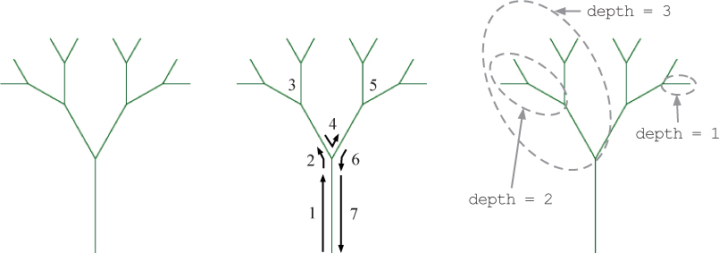
Figure 10.2 A tree produced by tree(george, 100, 4). The center figure illustrates what is drawn by each numbered step of the function. The figure on the right illustrates the self-similarity in the tree.
A fractal tree
An algorithm for creating a fractal shape is recursive, meaning that it invokes itself on smaller and smaller scales. Let’s consider the example of the simple tree shown on the left side of Figure 10.2. Notice that each of the two main branches of the tree is a smaller tree with the same structure as the whole. As illustrated in the center of Figure 10.2, to create this fractal tree, we first draw a trunk and then, for each branch, we draw two smaller trees at 30-degree angles using the same algorithm. Each of these smaller trees is composed of a trunk and two yet smaller trees, again drawn with the same tree-drawing algorithm. This process could theoretically continue forever, producing a tree with infinite complexity. In reality, however, the process eventually stops by invoking a non-recursive base case. The base case in Figure 10.2 is a “tree” that consists of only a single line segment.
This recursive structure is shown more precisely on the right side of Figure 10.2. The depth of the tree is a measure of its distance from the base case. The overall tree in Figure 10.2 has depth 4 and each of its two main branches is a tree with depth 3. Each of the two depth 3 trees is composed of two depth 2 trees. Finally, each of the four depth 2 trees is composed of two depth 1 trees, each of which is only a line segment.
The following tree function uses turtle graphics to draw this tree.
  import turtle

  def tree(tortoise, length, depth):
      """Recursively draw a tree.

      Parameters:
          tortoise: a Turtle object
          length: the length of the trunk
          depth: the desired depth of recursion

      Return value: None
      """

      if depth <= 1:                   # the base case
          tortoise.forward(length)
          tortoise.backward(length)
      else:                            # the recursive case
1         tortoise.forward(length)
2         tortoise.left(30)
3         tree(tortoise, length * (2 / 3), depth - 1)
4         tortoise.right(60)
5         tree(tortoise, length * (2 / 3), depth - 1)
6         tortoise.left(30)
7         tortoise.backward(length)

  def main():
      george = turtle.Turtle()
      george.left(90)
      tree(george, 100, 4)
      screen = george.getscreen()
      screen.exitonclick()

  main()
Let’s look at what happens when we run this program. The initial statements in the main function initialize the turtle and orient it to the north. Then the tree function is called with tree(george, 100, 4). On the lines numbered 1–2, the turtle moves forward length units to draw the trunk, and then turns 30 degrees to the left. This is illustrated in the center of Figure 10.2; the numbers correspond to the line numbers in the function. Next, to draw the smaller tree, we call the tree function recursively on line 3 with two-thirds of the length, and a value of depth that is one less than what was passed in. The depth parameter controls how long we continue to draw smaller trees recursively. After the call to tree returns, the turtle turns 60 degrees to the right on line 4 to orient itself to draw the right tree. On line 5, we recursively call the tree function again with arguments that are identical to those on line 3. When that call returns, the turtle retraces its steps in lines 6–7 to return to the origin.
The case when depth is at most 1 is called the base case because it does not make a recursive call to the function; this is where the recursion stops.
Reflection 10.1 Try running the tree-growing function with a variety of parameters. Also, try changing the turn angles and the amount length is shortened. Do you understand the results you observe?
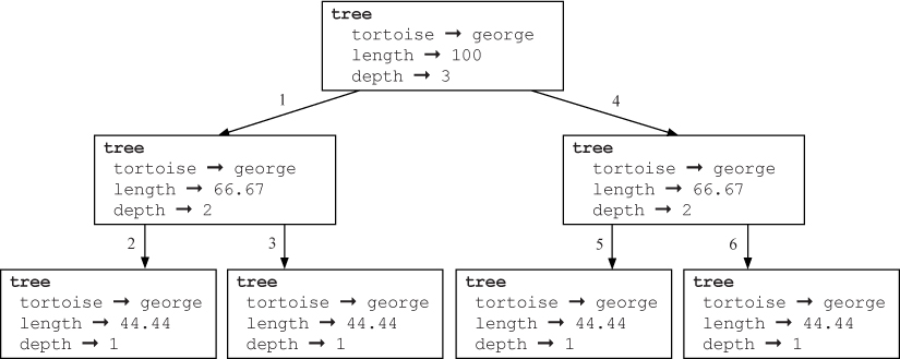
Figure 10.3 illustrates the recursive function calls that are made by the tree function when length is 100 and depth is 3. The top box represents a call to the tree function with parameters tortoise = george, length = 100, and depth = 3. This function calls two instances of tree with length = 100 * (2 / 3) = 66.67 and depth = 2. Then, each of these instances of tree calls two instances of tree with length = 66.67 * (2 / 3) = 44.44 and depth = 1. Because depth is 1, each of these instances of tree simply draws a line segment and returns.
Reflection 10.2 The numbers on the lines in Figure 10.3 represent the order in which the recursive calls are made. Can you see why that is?
Reflection 10.3 What would happen if we removed the base case from the algorithm by deleting the first four statements, so that the line numbered 1 was always the first statement executed?
The base case is extremely important to the correctness of this algorithm. Without the base case, the function would continue to make recursive calls forever!
A fractal snowflake
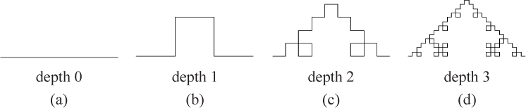
One of the most famous fractal shapes is the Koch curve, named after Swedish mathematician Helge von Koch. A Koch curve begins with a single line segment with length ℓ. Then that line segment is divided into three equal parts, each with length ℓ/3. The middle part of this divided segment is replaced by two sides of an equilateral triangle (with side length ℓ/3), as depicted in Figure 10.4(b). Next, each of the four line segments of length ℓ/3 is divided in the same way, with the middle segment again replaced by two sides of an equilateral triangle with side length ℓ/9, etc., as shown in Figure 10.4(c)–(d). As with the tree above, this process could theoretically go on forever, producing an infinitely intricate pattern.
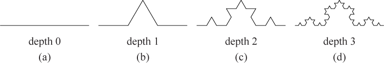
Notice that, like the tree, this shape exhibits self-similarity; each “side” of the Koch curve is itself a Koch curve with smaller depth. Consider first the Koch curve in Figure 10.4 with depth 1. It consists of four smaller Koch curves with depth 0 and length ℓ/3. Likewise, the Koch curve with depth 2 consists of four smaller Koch curves with depth 1 and the Koch curve with depth 3 consists of four smaller Koch curves with depth 2.
We can use our understanding of this self-similarity to write an algorithm to produce a Koch curve. To draw a Koch curve with depth d (d > 0) and overall horizontal length ℓ, we do the following:
Draw a Koch curve with depth d – 1 and overall length ℓ/3.
Turn left 60 degrees.
Draw another Koch curve with depth d – 1 and overall length ℓ/3.
Turn right 120 degrees.
Draw another Koch curve with depth d – 1 and overall length ℓ/3.
Turn left 60 degrees.
Draw another Koch curve with depth d – 1 and overall length ℓ/3.
The base case occurs when d = 0. In this case, we simply draw a line with length ℓ.
Reflection 10.4 Follow the algorithm above to draw (on paper) a Koch curve with depth 1. Then follow the algorithm again to draw one with depth 2.
This algorithm can be directly translated into Python:
def koch(tortoise, length, depth):
    """Recursively draw a Koch curve.

    Parameters:
        tortoise: a Turtle object
        length: the length of a line segment
        depth: the desired depth of recursion

    Return value: None
    """

    if depth == 0:                             # base case
        tortoise.forward(length)
    else:                                      # recursive case
        koch(tortoise, length / 3, depth - 1)
        tortoise.left(60)
        koch(tortoise, length / 3, depth - 1)
        tortoise.right(120)
        koch(tortoise, length / 3, depth - 1)
        tortoise.left(60)
        koch(tortoise, length / 3, depth - 1)

def main():
    george = turtle.Turtle()
    koch(george, 400, 3)
    screen = george.getscreen()
    screen.exitonclick()

main()
Reflection 10.5 Run this program and experiment by calling koch with different values of length and depth.
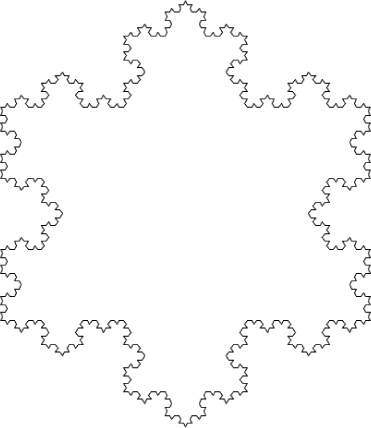
We can attach three Koch curves at 120-degree angles to produce an intricate snowflake shape like that in Figure 10.5.
Reflection 10.6 Look carefully at Figure 10.5. Can you see where the three individual Koch curves are connected?
The following function draws this Koch snowflake.
def kochSnowFlake(tortoise, length, depth):
    """Recursively draw a Koch snowflake.

    Parameters:
        tortoise: a Turtle object
        length: the length of a line segment
        depth: the desired depth of recursion

    Return value: None
    """

    for side in range(3):
        koch(tortoise, length, depth)
        tortoise.right(120)
Reflection 10.7 Insert this function into the previous program and call it from main. Try making different snowflakes by increasing the number of sides (and decreasing the right turn angle).
Imagine a Koch snowflake made from infinitely recursive Koch curves. Paradoxically, while the area inside any Koch snowflake is clearly finite (because it is bounded), the length of its border is infinite! In fact, the distance between any two points on its border is infinite! To see this, notice that, at every stage in its construction, each line segment is replaced with four line segments that are one-third the length of the original. Therefore, the total length of that “side” increases by one-third. Since this happens infinitely often, the perimeter of the snowflake continues to grow forever.

Exercises
10.1.1. Modify the recursive tree-growing function so that it branches at random angles between 10 and 60 degrees (instead of 30 degrees) and it shrinks the trunk/branch length by a random fraction between 0.5 and 0.75. Do your new trees now look more “natural”?
10.1.2. The quadratic Koch curve is similar to the Koch curve, but replaces the middle segment of each side with three sides of a square instead, as illustrated in Figure 10.6. Write a recursive function
quadkoch(tortoise, length, depth)
that draws the quadratic Koch curve with the given segment length and depth.
10.1.3. Each of the following activities is recursive in the sense that each step can be considered a smaller version of the original activity. Describe how this is the case and how the “input” gets smaller each time. What is the base case of each operation below?
- Evaluating an arithmetic expression like 7 + (15 – 3)/4.
- The chain rule in calculus (if you have taken calculus).
- One hole of golf.
- Driving directions to some destination.
10.1.4. Generalize the Koch snowflake function with an additional parameter so that it can be used to draw a snowflake with any number of sides.

10.1.5. The Sierpinski triangle, depicted in Figure 10.7, is another famous fractal. The fractal at depth 0 is simply an equilateral triangle. The triangle at depth 1 is composed of three smaller triangles, as shown in Figure 10.7(b). (The larger outer triangle and the inner “upside down” triangle are indirect effects of the positions of these three triangles.) At depth 2, each of these three triangles is replaced by three smaller triangles. And so on. Write a recursive function
sierpinski(tortoise, p1, p2, p3, depth)
that draws a Sierpinski triangle with the given depth. The triangle’s three corners should be at coordinates p1, p2, and p3 (all tuples). It will be helpful to also write two smaller functions that you can call from sierpinski: one to draw a simple triangle, given the coordinates of its three corners, and one to compute the midpoint of a line segment.
10.1.6. The Hilbert space-filling curve, shown in Figure 10.8, is a fractal path that visits all of the cells in a square grid in such a way that close cells are visited close together in time. For example, the figure below shows how a depth 2 Hilbert curve visits the cells in an 8 × 8 grid.

Assume the turtle is initially pointing north (up). Then the following algorithm draws a Hilbert curve with depth d >= 0. The algorithm can be in one of two different modes. In the first mode, steps 1 and 11 turn right, and steps 4 and 8 turn left. In the other mode, these directions are reversed (indicated in square brackets below). Steps 2 and 10 make recursive calls that switch this mode.

Figure 10.9 Sierpinski carpets with depths 0, 1, and 2. (The gray bounding box shows the extent of the drawing area; it is not actually part of the fractal.)
Turn 90 degrees to the right [left].
Draw a depth d – 1 Hilbert curve with left/right swapped.
Draw a line segment.
Turn 90 degrees to the left [right].
Draw a depth d – 1 Hilbert curve.
Draw a line segment.
Draw a depth d – 1 Hilbert curve.
Turn 90 degrees to the left [right].
Draw a line segment.
Draw a depth d – 1 Hilbert curve with left and right swapped.
Turn 90 degrees to the right [left].
The base case of this algorithm (d < 0) draws nothing. Write a recursive function
hilbert(tortoise, reverse, depth)
that draws a Hilbert space-filling curve with the given depth. The Boolean parameter reverse indicates which mode the algorithm should draw in. (Think about how you can accommodate both drawing modes by changing the angle of the turns.)
10.1.7. A fractal pattern called the Sierpinski carpet is shown in Figure 10.9. At depth 0, it is simply a filled square one-third the width of the overall square space containing the fractal. At depth 1, this center square is surrounded by eight one-third size Sierpinski carpets with depth 0. At depth 2, the center square is surrounded by eight one-third size Sierpinski carpets with depth 1. Write a function
carpet(tortoise, upperLeft, width, depth)

that draws a Sierpinski carpet with the given depth. The parameter upperLeft refers to the coordinates of the upper left corner of the fractal and width refers to the overall width of the fractal.
10.1.8. Modify your Sierpinski carpet function from the last exercise so that it displays the color pattern shown in Figure 10.10.
10.2 RECURSION AND ITERATION
We typically only solve problems recursively when they obviously exhibit self-similarity or seem “naturally recursive,” as with fractals. But recursion is not some obscure problem-solving technique. Although recursive algorithms may seem quite different from iterative algorithms, recursion and iteration are actually just two sides of the same coin. Every iterative algorithm can be written recursively, and vice versa. This realization may help take some of the mystery out of this seemingly foreign technique.
Consider the problem of summing the numbers in a list. Of course, this is easily achieved iteratively with a for loop:
def sumList(data):
    """Compute the sum of the values in a list.

    Parameter:
        data: a list of numbers

    Return value: the sum of the values in the list
    """

    sum = 0
    for value in data:
        sum = sum + value
    return sum
Let’s think about how we could achieve the same thing recursively. To solve a problem recursively, we need to think about how we could solve it if we had a solution to a smaller subproblem. A subproblem is the same as the original problem, but with only part of the original input.
In the case of summing the numbers in a list named data, a subproblem would be summing the numbers in a slice of data. Consider the following example:

If we had the sum of the numbers in data[1:], i.e., sumList(data[1:]), then we could compute the value of sumList(data) by simply adding this sum to data[0]. In other words, sumList(data) is equal to data[0] plus the solution to the subproblem sumList(data[1:]). In terms of the example above, if we knew that sumList([7, 3, 6]) returned 16, then we could easily find that sumList([1, 7, 3, 6]) is 1 + 16 = 17.
Reflection 10.8 Will this work if data is empty?
Since there is no data[0] or data[1:] when data is empty, the method above will not work in this case. But we can easily check for this case and simply return 0; this is the base case of the function. Putting these two parts together, we have the following function:
def sumList(data):
    """ (docstring omitted) """

    if len(data) == 0:                  # base case
        return 0
    return data[0] + sumList(data[1:])  # recursive case
But does this actually work? Yes, it does. To see why, let’s look at Figure 10.11. At the top of the diagram, in box (a), is a representation of a main function that has called sumList with the argument [1, 7, 3, 6]. Calling sumList creates a new instance of the sumList function, represented in box (b), with data assigned the values [1, 7, 3, 6]. Since data is not empty, the function will return 1 + sumList([7, 3, 6]), the value enclosed in the gray box. To evaluate this return value, we must call sumList again with the argument [7, 3, 6], resulting in another instance of the sumList function, represented in box (c). The instance of sumList in box (b) must wait to return its value until the instance in box (c) returns. Again, since data is not empty, the instance of sumList in box (c) will return 7 + sumList([3, 6]). Evaluating this value requires that we call sumList again, resulting in the instance of sumList in box (d). This process continues until the instance of sumList in box (e) calls sumList([]), creating the instance of sumList in box (f). Since this value of the data parameter is empty, the instance of sumList in box (f) immediately returns 0 to the instance of sumList that called it, in box (e). Now that the instance of sumList in box (e) has a value for sumList([]), it can return 6 + 0 = 6 to the instance of sumList in box (d). Since the instance of sumList in box (d) now has a value for sumList([6]), it can return 3 + 6 = 9 to the instance of sumList in box (c). The process continues up the chain until the value 17 is finally returned to main.
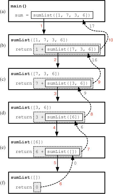
Figure 10.11 A representation of the function calls in the recursive sumList function. The red numbers indicate the order in which the events occur. The black numbers next to the arrows are return values.
Notice that the sequence of function calls, moving down the figure from (a) to (f), only ended because we eventually reached the base case in which data is empty, which resulted in the function returning without making another recursive call. Every recursive function must have a non-recursive base case, and each recursive call must get one step closer to the base case. This may sound familiar; it is very similar to the way we must think about while loops. Each iteration of a while loop must move one step closer to the loop condition becoming false.
Solving a problem recursively
The following five questions generalize the process we followed to design the recursive sumList function. We will illustrate each question by summarizing how we answered it in the design of the sumList.
What does a subproblem look like?
A subproblem is to compute the sum of a slice of the list.
Suppose we could ask an all-knowing oracle for the solution to any subproblem (but not for the solution to the problem itself). Which subproblem solution would be the most useful for solving the original problem?
The most useful solution would be the solution for a sublist that contains all but one element of the original list, e.g.,
sumList(data[1:]).How do we find the solution to the original problem using this subproblem solution? Implement this as the recursive step of our recursive function.
The solution to
sumList(data)isdata[0] + sumList(data[1:]). Therefore, the recursive step in our function should bereturn data[0] + sumList(data[1:])
What are the simplest subproblems that we can solve non-recursively, and what are their solutions? Implement your answer as the base case of the recursive function.
The simplest subproblem would be to compute the sum of an empty list, which is 0, of course. So the base case should be
if len(data) == 0:
    return 0
For any possible parameter value, will the recursive calls eventually reach the base case?
Yes, since an empty list will obviously reach the base case and any other list will result in a sequence of recursive calls that each involve a list that is one element shorter.
Reflection 10.9 How could we have answered question 2 differently? What is another subproblem that involves all but one element of the original list? Using this subproblem instead, answer the rest of the questions to write an alternative recursive sumList function.
An alternative subproblem that involves all but one element would be sumList(data[:-1]) (all but the last element). Then the solution to the original problem would be sumList(data[:-1]) + data[-1]. The base case is the same, so the complete function is
def sumList(data):
    """ (docstring omitted) """

    if len(data) == 0:                   # base case
        return 0
    return sumList(data[:-1]) + data[-1] # recursive case
Palindromes
Let’s look at another example. A palindrome is any sequence of characters that reads the same forward and backward. For example, radar, star rats, and now I won are all palindromes. An iterative function that determines whether a string is a palindrome is shown below.
def palindrome(s):
    """Determine whether a string is a palindrome.

    Parameter: a string s

    Return value: a Boolean value indicating whether s is a palindrome
    """

    for index in range(len(s) // 2):
        if s[index] != s[-(index + 1)]:
            return False
    return True
Let’s answer the five questions above to develop an equivalent recursive algorithm for this problem.
Reflection 10.10 First, what does a subproblem look like?
A subproblem would be to determine whether a slice of the string (i.e., a substring) is a palindrome.
Reflection 10.11 Second, if you could know whether any slice is a palindrome, which would be the most helpful?
It is often helpful to look at an example. Consider the following:
![]()
If we begin by looking at the first and last characters and determine that they are not the same, then we know that the string is not a palindrome. But if they are the same, then the question of whether the string is a palindrome is decided by whether the slice that omits the first and last characters, i.e., s[1:-1], is a palindrome. So it would be helpful to know the result of palindrome(s[1:-1]).
Reflection 10.12 Third, how could we use this information to determine whether the whole string is a palindrome?
If the first and last characters are the same and s[1:-1] is a palindrome, then s is a palindrome. Otherwise, s is not a palindrome. In other words, our desired return value is the answer to the following Boolean expression.
return s[0] == s[-1] and palindrome(s[1:-1])
If the first part is true, then the answer depends on whether the slice is a palindrome (palindrome(s[1:-1])). Otherwise, if the first part is false, then the entire and expression is false. Furthermore, due to the short circuit evaluation of the and operator, the recursive call to palindrome will be skipped.
Reflection 10.13 What are the simplest subproblems that we can solve non-recursively, and what are their solutions? Implement your answer as the base case.
The simplest string is, of course, the empty string, which we can consider a palindrome. But strings containing a single character are also palindromes, since they read the same forward and backward. So we know that any string with length at most one is a palindrome. But we also need to think about strings that are obviously not palindromes. Our discussion above already touched on this; when the first and last characters are different, we know that the string cannot be a palindrome. Since this situation is already handled by the Boolean expression above, we do not need a separate base case for it.
Putting this all together, we have the following elegant recursive function:
def palindrome(s):
    """ (docstring omitted) """

    if len(s) <= 1:    # base case
        return True
    return s[0] == s[-1] and palindrome(s[1:-1])
Let’s look more closely at how this recursive function works. On the left side of Figure 10.12 is a representation of the recursive calls that are made when the palindrome function is called with the argument 'now I won'. From the main function in box (a), palindrome is called with 'now I won', creating the instance of palindrome in box (b). Since the first and last characters of the parameter are equal (the s[0] == s[-1] part of the return statement is not shown to make the pictures less cluttered), the function will return the value of palindrome('ow I wo'). But, in order to get this value, it needs to call palindrome again, creating the instance in box (c). These recursive calls continue until we reach the base case in box (f), where the length of the parameter is one. The instance of palindrome in box (f) returns True to the previous instance of palindrome in box (e). Now the instance in box (e) returns to (d) the value True that it just received from (f). The value of True is propagated in this way all the way up the chain until it eventually reaches main, where it is assigned to the variable named pal.
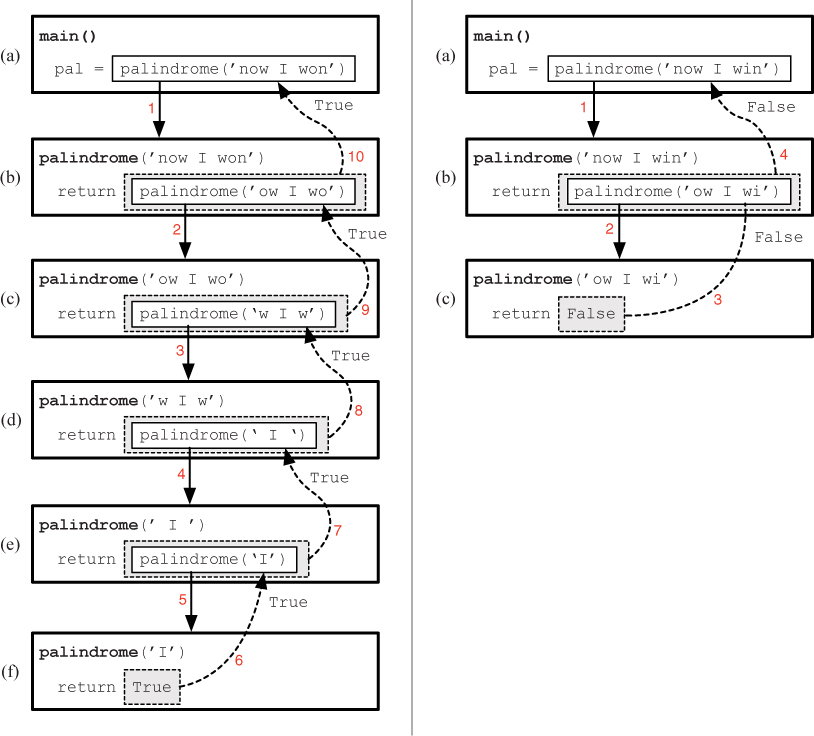
Figure 10.12 A representation of the function calls in the recursive palindrome function. The red numbers indicate the order in which the events happen. On the left is an instance in which the function reaches the base case and returns True. On the right is an instance in which the function returns False.
To see how the function returns False, let’s consider the example on the right side of Figure 10.12. In this example, the recursive palindrome function is called from main in box (a) with the non-palindromic argument 'now I win', which creates the instance of palindrome in box (b). As before, since the first and last characters of the parameter are equal, the function will return the value of palindrome('ow I wi'). Calling palindrome with this parameter creates the instance in box (c). But now, since the first and last characters of the parameter are not equal, Boolean expression returned by the function is False, so the instance of palindrome in box (c) returns False, and this value is propagated up to the main function.
Guessing passwords
One technique that hackers use to compromise computer systems is to rapidly try all possible passwords up to some given length.
Reflection 10.14 How many possible passwords are there with length n, if there are c possible characters to choose from?
The number of different passwords with length n is

For example, there are
268 = 208, 827, 064, 576 ≈ 208 billion
different eight-character passwords that use only lower-case letters. But there are
6712 = 8, 182, 718, 904, 632, 857, 144, 561 ≈ 8 sextillion
different twelve-character passwords that draw from the lower and upper-case letters, digits, and the five special characters $, &, #, ?, and !, which is why web sites prompt you to use long passwords with all of these types of characters! When you use a long enough password and enough different characters, this “guess and check” method is useless.
Let’s think about how we could generate a list of possible passwords by first considering the simpler problem of generating all binary strings (or “bit strings”) of a given length. This is the same problem, but using only two characters: '0' and '1'. For example, the list of all binary strings with length three is ['000', '001', '010', '011', '100', '101', '110', '111'].
Thinking about this problem iteratively can be daunting. However, it becomes easier if we think about the problem’s relationship to smaller versions of itself (i.e., self-similarity). As shown below, a list of binary strings with a particular length can be created easily if we already have a list of binary strings that are one bit shorter. We simply make two copies of the list of shorter binary strings, and then precede all of the strings in the first copy with a 0 and all of the strings in the second copy with a 1.

In the illustration above, the list of binary strings with length 2 is created from two copies of the list of binary strings with length 1. Then the list of binary strings with length 3 is created from two copies of the list of binary strings with length 2. In general, the list of all binary strings with a given length is the concatenation of
- the list of all binary strings that are one bit shorter and preceded by zero and
- the list of all binary strings that are one bit shorter and preceded by one.
Reflection 10.15 What is the base case of this algorithm?
The base case occurs when the length is 0, and there are no binary strings. However, the problem says that the return value should be a list of strings, so we will return a list containing an empty string in this case. The following function implements our recursive algorithm:
def binary(length):
    """Return a list of all binary strings with the given length.

    Parameter:
        length: the length of the binary strings

    Return value:
        a list of all binary strings with the given length
    """

    if length == 0:                          # base case
        return ['']

    shorter = binary(length - 1)  # recursively get shorter strings

    bitStrings = []                           # create a list
    for shortString in shorter:               #   of bit strings
        bitStrings.append('0' + shortString)  #   with prefix 0
    for shortString in shorter:               # append bit strings
        bitStrings.append('1' + shortString)  #   with prefix 1

    return bitStrings                         # return all bit strings
In the recursive step, we assign a list of all bit strings with length that is one shorter to shorter, and then create two lists of bit strings with the desired length. The first, named bitStrings0, is a list of bit strings consisting of each bit string in shorter, preceded by '0'. Likewise, the second list, named bitStrings1, contains the shorter bit strings preceded by '1'. The return value is the list consisting of the concatenation of bitStrings0 and bitStrings1.
Reflection 10.16 Why will this algorithm not work if we return an empty list ([ ]) in the base case? What will be returned?
If we return an empty list in the base case instead of a list containing an empty string, the function will return an empty list. To see why, consider what happens when we call binary(1). Then shorter will be assigned the empty list, which means that there is nothing to iterate over in the two for loops, and the function returns the empty list. Since binary(2) calls binary(1), this means that binary(2) will also return the empty list, and so on for any value of length!
Reflection 10.17 Reflecting the algorithm we developed, the function above contains two nearly identical for loops, one for the '0' prefix and one for the '1' prefix. How can we combine these two loops?
We can combine the two loops by repeating a more generic version of the loop for each of the characters '0' and '1':
def binary(length):
    """ (docstring omitted) """

    if length == 0:
        return ['']

    shorter = binary(length - 1)

    bitStrings = []
    for character in ['0', '1']:
        for shortString in shorter:
            bitStrings.append(character + shortString)

    return bitStrings
We can use a very similar algorithm to generate a list of possible passwords. The only difference is that, instead of preceding each shorter string with 0 and 1, we need to precede each shorter string with every character in the set of allowable characters. The following function, with a string of allowable characters assigned to an additional parameter, is a simple generalization of our binary function.
def passwords(length, characters):
    """Return a list of all possible passwords with the given length,
       using the given characters.

      Parameters:
          length: the length of the passwords
          characters: a string containing the characters to use

      Return value:
          a list of all possible passwords with the given length,
          using the given characters
      """

      if length == 0:
          return ['']

      shorter = passwords(length - 1, characters)

      passwordList = []
      for character in characters:
          for shorterPassword in shorter:
              passwordList.append(character + shorterPassword)

      return passwordList
Reflection 10.18 How would we call the passwords function to generate a list of all bit strings with length 5? What about all passwords with length 4 containing the characters 'abc123'? What about all passwords with length 8 containing lower case letters? (Do not actually try this last one!)
Exercises
Write a recursive function for each of the following problems.
10.2.1. Write a recursive function
sum(n)
that returns the sum of the integers from 1 to n.
10.2.2. Write a recursive function
factorial(n)
that returns the value of n! = 1 . 2 . 3 ..... n.
10.2.3. Write a recursive function
power(a, n)
that returns the value of an without using the ** operator.
10.2.4. Write a recursive function
minList(data)
that returns the minimum of the items in the list of numbers named data. You may use the built-in min function for finding the minimum of two numbers (only).
10.2.5. Write a recursive function
length(data)
that returns the length of the list data without using the len function.
10.2.6. Euclid’s algorithm for finding the greatest common divisor (GCD) of two integers uses the fact that the GCD of m and n is the same as the GCD of n and m mod n (the remainder after dividing m by n). Write a function
gcd(m, n)
that recursively implements Euclid’s GCD algorithm. For the base case, use the fact that gcd(m, 0) is m.
10.2.7. Write a recursive function
reverse(text)
that returns the reverse of the string named text.
10.2.8. Write a recursive function
int2string(n)
that converts an integer value n to its string equivalent, without using the str function. For example, int2string(1234) should return the string '1234'.
10.2.9. Write a recursive function
countUpper(s)
that returns the number of uppercase letters in the string s.
10.2.10. Write a recursive function
equal(list1, list2)
that returns a Boolean value indicating whether the two lists are equal without testing whether list1 == list2. You may only compare the lengths of the lists and test whether individual list elements are equal.
10.2.11. Write a recursive function
powerSet(n)
that returns a list of all subsets of the integers 1, 2, ..., n. A subset is a list of zero or more unique items from a set. The set of all subsets of a set is also called the power set. For example, subsets(n) should return the list [[], [1], [2], [2, 1], [3], [3, 1], [3, 2], [3, 2, 1]]. (Hint: this is similar to the binary function.)

10.2.12. Suppose you work for a state in which all vehicle license plates consist of a string of letters followed by a string of numbers, such as 'ABC 123'. Write a recursive function
licensePlates(length, letters, numbers)
that returns a list of strings representing all possible license plates of this form, with length letters and numbers chosen from the given strings. For example, licensePlates(2, 'XY', '12') should return the following list of 16 possible license plates consisting of two letters drawn from 'XY' followed by two digits drawn from '12':
['XX 11', 'XX 21', 'XY 11', 'XY 21', 'XX 12', 'XX 22',
 'XY 12', 'XY 22', 'YX 11', 'YX 21', 'YY 11', 'YY 21',
 'YX 12', 'YX 22', 'YY 12', 'YY 22']
(Hint: this is similar to the passwords function.)
10.3 THE MYTHICAL TOWER OF HANOI
The Tower of Hanoi is a game that was first marketed in 1883 by French mathematician Édouard Lucas. As illustrated in Figure 10.13, the game is played on a board with three pegs. One peg holds some number of disks with unique diameters, ordered smallest to largest. The objective of the game is to move this “tower” of disks from their original peg to another peg, one at a time, without ever placing a larger disk on top of a smaller one. The game was purported to have originated in an ancient legend. In part, the game’s instruction sheet reads:
According to an old Indian legend, the Brahmins have been following each other for a very long time on the steps of the altar in the Temple of Benares, carrying out the moving of the Sacred Tower of Brahma with sixty-four levels in fine gold, trimmed with diamonds from Golconde. When all is finished, the Tower and the Brahmins will fall, and that will be the end of the world!1
This game is interesting because it is naturally solved using the following recursive insight. To move n disks from the first peg to the third peg, we must first be able to move the bottom (largest) disk on the first peg to the bottom position on the third peg. The only way to do this is to somehow move the top n – 1 disks from the first peg to the second peg, to get them out of the way, as illustrated in Figure 10.14(a)–(b). But notice that moving n – 1 disks is a subproblem of moving n disks because it is the same problem but with only part of the input. The source and destination pegs are different in the original problem and the subproblem, but this can be handled by making the source, destination, and intermediate pegs additional inputs to the problem. Because this step is a subproblem, we can perform it recursively! Once this is accomplished, we are free to move the largest disk from the first peg to the third peg, as in Figure 10.14(c). Finally, we can once again recursively move the n – 1 disks from the second peg to the third peg, shown in Figure 10.14(d). In summary, we have the following recursive algorithm:

Recursively move the top n – 1 disks from the source peg to the intermediate peg, as in Figure 10.14(b).
Move one disk from the source peg to the destination peg, as in Figure 10.14(c).
Recursively move the n – 1 disks from the intermediate peg to the destination peg, as in Figure 10.14(d).
Reflection 10.19 What is the base case in this recursive algorithm? In other words, what is the simplest subproblem that will be reached by these recursive calls?
The simplest base case would be if there were no disks at all! In this case, we simply do nothing.
We cannot actually write a Python function to move the disks for us, but we can write a function that gives us instructions on how to do so. The following function accomplishes this, following exactly the algorithm described above.
      def hanoi(n, source, destination, intermediate):
          """Print instructions for solving the Tower of Hanoi puzzle.

          Parameters:
              n: the number of disks
              source: the source peg
              destination: the destination peg
              intermediate: the other peg

          Return value: None
          """

          if n >= 1:
              hanoi(n - 1, source, intermediate, destination)
              print('Move a disk from peg', source, 'to peg', destination)
              hanoi(n - 1, intermediate, destination, source)
The parameters n, source, destination, and intermediate represent the number of disks, the source peg, the destination peg, and the remaining peg that can be used as a temporary resting place for disks that we need to get out of the way. In our examples, peg 1 was the source, peg 3 was the destination, and peg 2 was the intermediate peg. Notice that the base case is implicit: if n is less than one, the function simply returns.
When we execute this function, we can name our pegs anything we want. For example, if we name our pegs A, B, and C, then
hanoi(8, 'A', 'C', 'B')
will print instructions for moving eight disks from peg A to peg C, using peg B as the intermediate.
Reflection 10.20 Execute the function with three disks. Does it work? How many steps are necessary? What about with four and five disks? Do you see a pattern?
*Is the end of the world nigh?
The original game’s instruction sheet claimed that the world would end when the monks finished moving 64 disks. So how long does this take? To derive a general answer, let’s start by looking at small numbers of disks. When there is one disk, only one move is necessary: move the disk from the source peg to the destination peg. When there are two disks, the algorithm moves the smaller disk to the intermediate peg, then the larger disk to the destination peg, and finally the smaller disk to the destination peg, for a total of three moves.
When n is three, we need to first move the top two disks to the intermediate peg which, we just deduced, requires three moves. Then we move the largest disk to the destination peg, for a total of four moves so far. Finally, we move the two disks from the intermediate peg to the destination peg, which requires another three moves, for a total of seven moves.
In general, notice that the number of moves required for n disks is the number of moves required for n – 1 disks, plus one move for the bottom disk, plus the number of moves required for n – 1 disks again. In other words, if the function M(n) represents the number of moves required for n disks, then
M(n) = M(n – 1) + 1 + M(n – 1) = 2M(n – 1) + 1.
Does this look familiar? This is a difference equation, just like those in Chapter 4. In this context, a function that is defined in terms of itself is also called a recurrence relation. The pattern produced by this recurrence relation is illustrated by the following table.
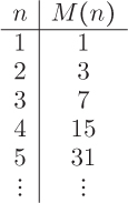
Reflection 10.21 Do you see the pattern in the table? What is the formula for M(n) in terms of n?
M(n) is always one less than 2n. In other words, the algorithm requires
M(n) = 2n – 1
moves to solve the the game when there are n disks. This expression is called a closed form for the recurrence relation because it is defined only in terms of n, not M(n – 1). According to our formula, moving 64 disks would require
264 – 1 = 18, 446, 744, 073, 709, 551, 615
moves. I guess the end of the world is not coming any time soon!
10.4 RECURSIVE LINEAR SEARCH
In Sections 6.5 and 8.5, we developed (and used) the fundamental linear search algorithm to find the index of a target item in a list. In this section, we will develop a recursive version of this function and then show that it has the same time complexity as the iterative version. Later, in Section 11.1, we will develop a more efficient algorithm for searching in a sorted list.
Reflection 10.22 What does a subproblem look like in the search problem? What would be the most useful subproblem to have an answer for?
In the search problem, a subproblem is to search for the target item in a smaller list. Since we can only “look at” one item at a time, the most useful subproblem will be to search for the target item in a sublist that contains all but one item. This way, we can break the original problem into two parts: determine if the target is this one item and determine if the target is in the rest of the list. It will be convenient to have this one item be the first item, so we can then solve the subproblem with the slice starting at index 1. Of course, if the first item is the one we are searching for, we can avoid the recursive call altogether. Otherwise, we return the index that is returned by the search of the smaller list.
Reflection 10.23 What is the base case for this problem?
We have already discussed one base case: if the target item is the first item in the list, we simply return its index. Another base case would be when the list is empty. In this case, the item for which we are searching is not in the list, so we return –1. The following function (almost) implements the recursive algorithm we have described.
def linearSearch(data, target):
    """Recursively find the index of the first occurrence of
       target in data.

    Parameters:
        data: a list object to search in
        target: an object to search for

    Return value: index of the first occurrence of target in data
    """

    if len(data) == 0:                     # base case 1: not found
        return -1
    if target == data[0]:                  # base case 2: found
        return ??
    return linearSearch(data[1:], target)  # recursive case
However, as indicated by the red question marks above, we have a problem.
Reflection 10.24 What is the problem indicated by the red question marks? Why can we not just return 0 in that case?
When we find the target at the beginning of the list and are ready to return its index in the original list, we do not know what it was! We know that it is at index 0 in the current sublist being searched, but we have no way of knowing where this sublist starts in the original list. Therefore, we need to add a third parameter to the function that keeps track of the original index of the first item in the sublist data. In each recursive call, we add one to this argument since the index of the new front item in the list will be one more than that of the current front item.
def linearSearch(data, target, first):
    """ (docstring omitted) """

    if len(data) == 0:                      # base case 1: not found
        return -1
    if target == data[0]:                   # base case 2: found
        return first
    return linearSearch(data[1:], target, first + 1) # recursive case
With this third parameter, we need to now initially call the function like
position = linearSearch(data, target, 0)
We can now also make this function more efficient by eliminating the need to take slices of the list in each recursive call. Since we now have the index of the first item in the sublist under consideration, we can pass the entire list as a parameter each time and use the value of first in the second base case.
def linearSearch(data, target, first):
    """ (docstring omitted) """

    if (first < 0) or (first >= len(data)):  # base case 1: not found
        return -1
    if target == data[first]:                # base case 2: found
        return first
    return linearSearch(data, target, first + 1) # recursive case
As shown above, this change also necessitates a change in our first base case because the length of the list is no longer decreasing to zero. Since the intent of the function is to search in the list between indices first and len(data) - 1, we will consider the list under consideration to be empty if the value of first is greater than the last index in the list. Just to be safe, we also make sure that first is at least zero.
Efficiency of recursive linear search
Like the iterative linear search, this algorithm has linear time complexity. But we cannot derive this result in the same way we did for the iterative version. Instead, we need to use a recurrence relation, as we did to find the number of moves required in the Tower of Hanoi algorithm.
Let T(n) represent the maximum (worst case) number of comparisons required by a linear search when the length of the list is n. When we look at the algorithm above, we see that there are two comparisons that the algorithm must make before reaching a recursive function call. But since it only matters asymptotically that this number is a constant, we will simply represent the number of comparisons before the recursive call as a constant value c. Therefore, the number of comparisons necessary in the base case in which the list is empty (n = 0) is T(0) = c. In recursive cases, there are additional comparisons to be made in the recursive call.
Reflection 10.25 How many more comparisons are made in the recursive call to linearSearch?
The size of the sublist yet to be considered in each recursive call is n – 1, one less than in the current instance of the function. Therefore, the number of comparisons in each recursive call must be the number of comparisons required by a linear search on a list with length n – 1, which is T(n – 1). So the total number of comparisons is
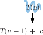
T(n) = T(n – 1) + c.
But this is not very helpful in determining what the time complexity of the linear search is. To get this recurrence relation into a more useful form, we can think about the recurrence relation as saying that the value of T(n) is equal to, or can be replaced by, the value of T(n – 1) + c, as illustrated below:
Reflection 10.26 Now what can we replace T(n – 1) with?
T(n – 1) is just T(n) with n – 1 substituted for n. Therefore, using the definition of T(n) above,
T(n – 1) = T(n – 1 – 1) + c = T(n – 2) + c.
So we can also substitute T(n – 2) + c for T(n – 1). Similarly,
T(n – 2) = T(n – 2 – 1) + c = T(n – 3) + c.
and
T(n – 3) = T(n – 3 – 1) + c = T(n – 4) + c.
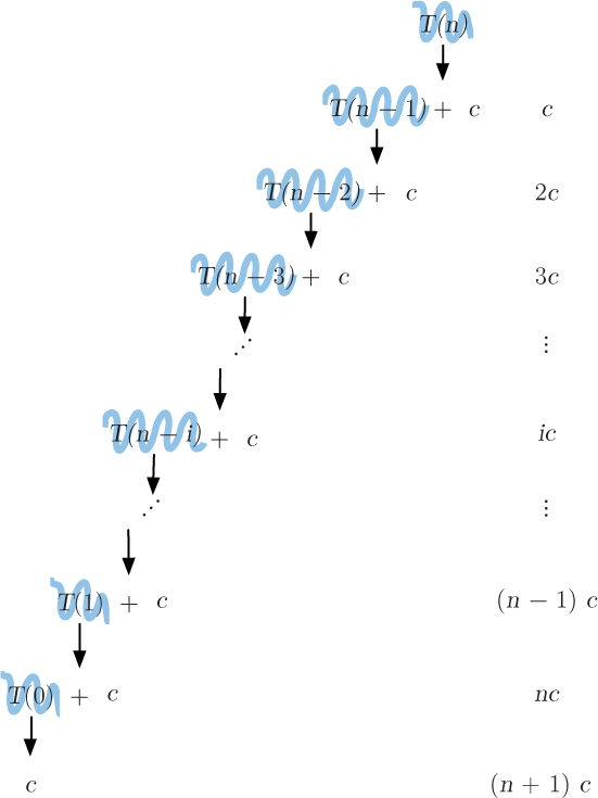
This sequence of substitutions is illustrated in Figure 10.15. The right side of the figure illustrates the accumulation of c’s as we proceed downward. Since c is the number of comparisons made before each recursive call, these values on the right represent the number of comparisons made so far. Notice that the number subtracted from n in the argument of T at each step is equal to the multiplier in front of the accumulated c’s at that step. In other words, to the right of each T(n – i), the accumulated value of c’s is i · c. When we finally reach T(0), which is the same as T(n – n), the total on the right must be nc. Finally, we showed above that T(0) = c, so the total number of comparisons is (n + 1)c. This expression is called the closed form of the recurrence relation because it does not involve any values of T(n). Since (n + 1)c is proportional to n asymptotically, recursive linear search is a linear-time algorithm, just like the iterative linear search. Intuitively, this should make sense because the two algorithms essentially do the same thing: they both look at every item in the list until the target is found.
Exercises
10.4.1. Our first version of the linearSearch function, without the first parameter, can work if we only need to know whether the target is contained in the list or not. Write a working version of this function that returns True if the target item is contained in the list and False otherwise.
10.4.2. Unlike our final version of the linearSearch function, the function you wrote in the previous exercise uses slicing. Is this still a linear-time algorithm?
10.4.3. Write a new version of recursive linear search that looks at the last item in the list, and recursively calls the function with the sublist not containing the last item instead.
10.4.4. Write a new version of recursive linear search that only looks at every other item in the list for the target value. For example, linearSearch([1, 2, 3, 4, 2], 2, 0) should return the index 4 because it would not find the target, 2, at index 1.
10.4.5. Write a recursive function
sumSearch(data, total, first)
that returns the first index in data, greater than or equal to first, for which the sum of the values in data[:index + 1] is greater than or equal to total. If the sum of all of the values in the list is less than total, the function should return –1. For example, sumSearch([2, 1, 4, 3], 4) returns index 2 because 2 + 1 + 4 ≥ 4 but 2 + 1 < 4.
10.5 DIVIDE AND CONQUER
The algorithm for the Tower of Hanoi game elegantly used recursion to divide the problem into three simpler subproblems: recursively move n – 1 disks, move one disk, and then recursively move n – 1 disks again. Such algorithms came to be called divide and conquer algorithms because they “divide” a hard problem into two or more subproblems, and then “conquer” each subproblem recursively with the same algorithm. The divide and conquer technique has been found to yield similarly elegant, and often quite efficient, algorithms for a wide variety of problems.
It is actually useful to think of divide and conquer algorithms as comprising three steps instead of two:
Divide the problem into two or more subproblems.
Conquer each subproblem recursively.
Combine the solutions to the subproblems into a solution for the original problem.
In the Tower of Hanoi algorithm, the “combine” step was essentially free. Once the subproblems had been solved, we were done. But other problems do require this step at the end.
In this section, we will look at three more relatively simple examples of problems that are solvable by divide and conquer algorithms.
Buy low, sell high
Suppose that you have created a model to predict the future daily closing prices of a particular stock. With a list of these daily stock prices, you would like to determine when to buy and sell the stock to maximize your profit. For example, when should you buy and sell if your model predicts that the stock will be priced as follows?

It is tempting to look for the minimum price ($3.18) and then look for the maximum price after that day. But this clearly does not work with this example. Even choosing the second smallest price ($3.21) does not give the optimal answer. The most profitable choice is to buy on day 2 at $3.60 and sell on day 6 at $4.95, for a profit of $1.35 per share.
One way to find this answer is to look at all possible pairs of buy and sell dates, and pick the pair with the maximum profit. (See Exercise 8.5.5.) Since there are n(n – 1)/2 such pairs, this yields an algorithm with time complexity n2. However, there is a more efficient way. Consider dividing the list of prices into two equal-size lists (or as close as possible). Then the optimal pair of dates must either reside in the left half of the list, the right half of the list, or straddle the two halves, with the buy date in the left half and sell date in the right half. This observation can be used to design the following divide and conquer algorithm:
Divide the problem into two subproblems: (a) finding the optimal buy and sell dates in the left half of the list and (b) finding the optimal buy and sell dates in the right half of the list.
Conquer the two subproblems by executing the algorithm recursively on these two smaller lists of prices.
Combine the solutions by choosing the best buy and sell dates from the left half, the right half, and from those that straddle the two halves.
Reflection 10.27 Is there an easy way to find the best buy and sell dates that straddle the two halves, with the buy date in the left half and sell date in the right half?
At first glance, it might look like the “combine” step would require another recursive call to the algorithm. But finding the optimal buy and sell dates with this particular restriction is actually quite easy. The best buy date in the left half must be the one with the minimum price, and the best sell date in the right half must be the one with the maximum price. So finding these buy and sell dates simply amounts to finding the minimum price in the left half of the list and the maximum price in the right half, which we already know how to do.
Before we write a function to implement this algorithm, let’s apply it to the list of prices above:
[3.90, 3.60, 3.65, 3.71, 3.78, 4.95, 3.21, 4.50, 3.18, 3.53]
The algorithm divides the list into two halves, and recursively finds the maximum profit in the left list [3.90, 3.60, 3.65, 3.71, 3.78] and the maximum profit in the right list [4.95, 3.21, 4.50, 3.18, 3.53]. In each recursive call, the algorithm is executed again but, for now, let’s assume that we magically get these two maximum profits: 3.78 – 3.60 = 0.18 in the left half and 4.50 – 3.21 = 1.29 in the right half. Next, we find the maximum profit possible by holding the stock from the first half to the second half. Since the minimum price in the first half is 3.60 and the maximum price in the second half is 4.95, this profit is 1.35. Finally, we return the maximum of these three profits, which is 1.35.
Reflection 10.28 Since this is a recursive algorithm, we also need a base case. What is the simplest list in which to find the optimal buy and sell dates?
A simple case would be a list with only two prices. Then obviously the optimal buy and sell dates are days 1 and 2, as long as the price on day 2 is higher than the price on day 1. Otherwise, we are better off not buying at all (or equivalently, buying and selling on the same day). An even easier case would be a list with less than two prices; then once again we either never buy at all, or buy and sell on the same day.
The following function implements this divide and conquer algorithm, but just finds the optimal profit, not the actual buy and sell days. Finding these days requires just a little more work, which we leave for you to think about as an exercise.
 1 def profit(prices):
 2     """Find the maximum achievable profit from a list of daily
 3        stock prices.
 4
 5     Parameter:
 6         prices: a list of daily stock prices
 7
 8     Return value: the maximum profit
 9     """
10
11     if len(prices) <= 1:                        # base case
12         return 0
13
14     midIndex = len(prices) // 2                 # divide in half
15     leftProfit = profit(prices[:midIndex])      # conquer 2 halves
16     rightProfit = profit(prices[midIndex:])
17
18     buy = min(prices[:midIndex])                # min price on left
19     sell = max(prices[midIndex:])               # max price on right
20     midProfit = sell - buy
21     return max(leftProfit, rightProfit, midProfit) # combine 3 cases
The base case covers situations in which the list contains either one price or no prices. In these cases, the profit is 0. In the divide step, we find the index of the middle (or close to middle) price, which is the boundary between the left and right halves of the list. We then call the function recursively for each half. From each of these recursive calls, we get the maximum possible profits in the two halves. Finally, for the combine step, we find the minimum price in the left half of the list and the maximum price in the right half of the list. The final return value is then the maximum of the maximum profit from the left half of the list, the maximum profit from the right half of the list, and the maximum profit from holding the stock from a day in the first half to a day in the second half.
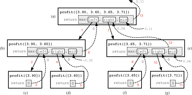
Figure 10.16 A representation of the function calls in the recursive profit function. The red numbers indicate the order in which the events happen.
Reflection 10.29 Call this function with the list of prices that we used in the example above.
That this algorithm actually works may seem like magic at this point. But, rest assured, like all recursive algorithms, there is a perfectly good reason why it works. The process is sketched out in Figure 10.16 for a small list containing just the first four prices in our example. As in Figures 10.11 and 10.12, each bold rectangle represents an instance of a function call. Each box contains the function’s name and argument, and a representation of how the return value is computed. In all but the base cases, this is the maximum of leftProfit (represented by left), rightProfit (represented by right), and midProfit (represented by mid). At the top of Figure 10.16, the profit function is called with a list of four prices. This results in calling profit recursively with the first two prices and the last two prices. The first recursive call (on line 15) is represented by box (b). This call to profit results in two more recursive calls, labeled (c) and (d), each of which is a base case. These two calls both return the value 0, which is separately assigned to leftProfit and rightProfit (left and right) in box (b). The profit from holding the stock in the combine step in box (b), -0.30, is assigned to midProfit (mid). And then the maximum value, which in this case is 0, is returned back to box (a) and assigned to leftProfit. Once this recursive call returns, the second recursive call (on line 16) is made from box (a), resulting in a similar sequence of function calls, as illustrated in boxes (e)–(g). This second recursive call from (a) results in 0.06 being assigned to rightProfit. Finally, the maximum of leftProfit, rightProfit, and midProfit, which is 3.71 - 3.60 = 0.11, is returned by the original function call. The red numbers on the arrows in the figure indicate the complete ordering of events.
Navigating a maze
Suppose we want to design an algorithm to navigate a robotic rover through an unknown, obstacle-filled terrain. For simplicity, we will assume that the landscape is laid out on a grid and the rover is only able to “see” and move to the four grid cells to its east, south, west, and north in each step, as long as they do not contain obstacles that the rover cannot move through.
To navigate the rover to its destination on the grid (or determine that the destination cannot be reached), we can use a technique called depth-first search. The depth-first search algorithm explores a grid by first exploring in one direction as far as it can from the source. Then it backtracks to follow paths that branch off in each of the other three directions. Put another way, a depth-first search divides the problem of searching for a path to the destination into four subproblems: search for a path starting from the cell to the east, search for a path starting from the cell to the south, search for a path starting from the cell to the west, and search for a path starting from the cell to the north. To solve each of these subproblems, the algorithm follows this identical procedure again, just from a different starting point. In terms of the three divide and conquer steps, the depth-first search algorithm looks like this:
Divide the problem into four subproblems. Each subproblem searches for a path that starts from one of the four neighboring cells.
Conquer the subproblems by recursively executing the algorithm from each of the neighboring cells.
Combine the solutions to the subproblems by returning success if any of the subproblems were successful. Otherwise, return failure.
To illustrate, consider the grid in Figure 10.17(a). In this example, we are attempting to find a path from the green cell in position (1, 1) to the red cell in position (3, 0). The black cells represent obstacles that we cannot move through. The depth-first search algorithm will visit neighboring cells in clockwise order: east, south, west, north. In the first step, the algorithm starts at cell (1, 1) and looks east to (1, 2), but cannot move in that direction due to an obstacle. Therefore, it next explores the cell to the south in position (2, 1), colored blue in Figure 10.17(b). From this cell, it recursively executes the same algorithm, first looking east to (2, 2). Since this cell is not blocked, it is the next one visited, as represented in Figure 10.17(c). The depth-first search algorithm is recursively called again from cell (2, 2), but the cells to the east, south, and north are blocked; and the cell to the west has already been visited. Therefore, the depth-first search algorithm returns failure to the cell at (2, 1). We color cell (2, 2) light blue to indicate that it has been visited, but is no longer on the path to the destination. From cell (2, 1), the algorithm has already looked east, so it now moves south to (3, 1), as shown in Figure 10.17(d). In the next step, shown in Figure 10.17(e), the algorithm moves south again to (4, 1) because the cell to the east is blocked.
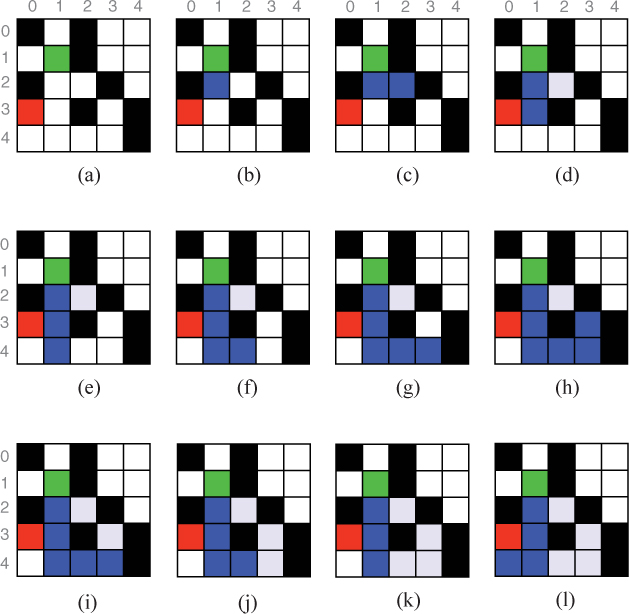
Reflection 10.30 When it is at cell (3, 1), why does the algorithm not “see” the destination in cell (3, 0)?
It does not yet “see” the destination because it looks east and south before it looks west. Since there is an open cell to the south, the algorithm will follow that possibility first. In the next steps, shown in Figure 10.17(f)–(g), the algorithm is able to move east, and in Figure 10.17(h), it is only able to move north. At this point, the algorithm backtracks to (4, 1) over three steps, as shown in Figure 10.17(i)–(k), because all possible directions have already been attempted from cells (3, 3), (4, 3), and (4, 2). From cell (4, 1), the algorithm next moves west to cell (4, 0), as shown in Figure 10.17(l), because it has already moved east and there is no cell to the south. Finally, from cell (4, 0), it cannot move east, south, or west; so it moves north where it finally finds the destination.
The final path shown in blue illustrates a path from the source to destination. Of course, this is not the path that the algorithm followed, but this path can now be remembered for future trips.
Reflection 10.31 Did the depth-first search algorithm find the shortest path?
A depth-first search is not guaranteed to find the shortest, or even a short, path. But it will find a path if one exists. Another algorithm, called a breadth-first search, can be used to find the shortest path.
Reflection 10.32 What is the base case of the depth-first search algorithm? For what types of source cells can the algorithm finish without making any recursive calls?
There are two kinds of base cases in depth-first search, corresponding to the two possible outcomes. One base case occurs when the source cell is not a “legal” cell from which to start a new search. These source cells are outside the grid, blocked, or already visited. In these cases, we simply return failure. The other base case occurs when the source cell is the same as the destination cell. In this case, we return success.
The depth-first search algorithm is implemented by the following function. The function returns True (success) if the destination was reached by a path and False (failure) if the destination could not be found.
BLOCKED = 0  # site is blocked
OPEN = 1     # site is open and not visited
VISITED = 2  # site is open and already visited

def dfs(grid, source, dest):
    """Perform a depth-first search on a grid to determine if there
       is a path between a source and destination.

    Parameters:
        grid: a 2D grid (list of lists)
        source: a (row, column) tuple to start from
        dest: a (row, column) tuple to reach

    Return value: Boolean indicating whether destination was reached
    """

    (row, col) = source
    rows = len(grid)
    columns = len(grid[0])

   if (row < 0) or (row >= rows)
     or (col < 0) or (col >= columns)
     or (grid[row][col] == BLOCKED)
     or (grid[row][col] == VISITED):    # dead end (base case)
       return False                     #   so return False

   if source == dest:                   # dest found (base case)
       return True                      #   so return True

   grid[row][col] = VISITED             # visit this cell

   if dfs(grid, (row, col + 1), dest):  # search east
       return True                      #  and return if dest found
   if dfs(grid, (row + 1, col), dest):  # else search   south
       return True                      #  and return if dest found
   if dfs(grid, (row, col - 1), dest):  # else search   west
       return True                      #  and return if dest found
   if dfs(grid, (row - 1, col), dest):  # else search   north
       return True                      #  and return if dest found

   return False                         # destination was not found
The variable names BLOCKED, VISITED, and OPEN represent the possible status of each cell. For example, the grid in Figure 10.17 is represented with
grid = [[BLOCKED, OPEN, BLOCKED, OPEN, OPEN],
        [OPEN, OPEN, BLOCKED, OPEN, OPEN],
        [BLOCKED, OPEN, OPEN, BLOCKED, OPEN],
        [OPEN, OPEN, BLOCKED, OPEN, BLOCKED],
        [OPEN, OPEN, OPEN, OPEN, BLOCKED]]
When a cell is visited, its value is changed from OPEN to VISITED by the dfs function. There is a program available on the book web site that includes additional turtle graphics code to visualize how the cells are visited in this depth-first search. Download this program and run it on several random grids.
Reflection 10.33 Our dfs function returns a Boolean value indicating whether the destination was reached, but it does not actually give us the path (as marked in blue in Figure 10.17). How can we modify the function to do this?
This modification is actually quite simple, although it may take some time to understand how it works. The idea is to add another parameter, a list named path, to which we append each cell after we mark it as visited. The values in this list contain the sequence of cells visited in the recursive calls. However, we remove the cell from path if we get to the end of the function where we return False because getting this far means that this cell is not part of a successful path after all. In our example in Figure 10.17, initially coloring a cell blue is analogous to appending that cell to the path, while recoloring a cell light blue when backtracking is analogous to removing the cell from the path. We leave an implementation of this change as an exercise. Two projects at the end of this chapter demonstrate how depth-first search can be used to solve other problems as well.
Exercises
Write a recursive divide and conquer function for each of the following problems. Each of your functions should contain at least two recursive calls.
10.5.1. Write a recursive divide and conquer function
power(a, n)
that returns the value of an, utilizing the fact that an = (an/2)2 when n is even and an = (a(n–1)/2)2 · a when n is odd. Assume that n is a non-negative integer.
10.5.2. The Fibonacci sequence is a sequence of integers in which each integer is the sum of the previous two. The first two Fibonacci numbers are 1, 1, so the sequence begins 1, 1, 2, 3, 5, 8, 13, .... Write a function
fibonacci(n)
that returns the nth Fibonacci number.
10.5.3. In the profit function, we defined the left half as ending at index midIndex - 1 and the right half starting at index midIndex. Would it also work to have the left half end at index midIndex and the right half start at index midIndex + 1? Why or why not?
10.5.4. The profit function in the text takes a single list as the parameter and calls the function recursively with slices of this list. In this exercise, you will write a more efficient version of this function
profit(prices, first, last)
that does not use slicing in the arguments to the recursive calls. Instead, the function will pass in the entire list in each recursive call, with the two additional parameters assigned the first and last indices of the sublist that we want to consider. In the divide step, the function will need to assign midIndex the index that is midway between first and last (which is usually not last // 2). To find the maximum profit achievable with a list of prices, the function must initially be called with profit(prices, 0, len(prices) - 1).
10.5.5. Modify the version of the function that you wrote in Exercise 10.5.4 so that it returns the most profitable buy and sell days instead of the maximum profit.
10.5.6. Write a divide and conquer version of the recursive linear search from Section 10.4 that checks if the middle item is equal to the target in each recursive call and then recursively calls the function with the first half and second half of the list, as needed. Your function should return the index in the list where the target value was found, or –1 if it was not found. If there are multiple instances of the target in the list, your function will not necessarily return the minimum index at which the target can be found. (This function is quite similar to Exercise 10.5.4.)
10.5.7. Write a new version of the depth-first search function
dfs(grid, source, dest, path)
in which the parameter path contains the sequence of cell coordinates that comprise a path from source to dest in the grid when the function returns. The initial value of path will be an empty list. In other words, to find the path in Figure 10.17, your function will be called like this:
grid = [[BLOCKED, OPEN, BLOCKED, OPEN, OPEN],
        [OPEN, OPEN, BLOCKED, OPEN, OPEN],
        [BLOCKED, OPEN, OPEN, BLOCKED, OPEN],
        [OPEN, OPEN, BLOCKED, OPEN, BLOCKED],
        [OPEN, OPEN, OPEN, OPEN, BLOCKED]]
path = []
success = dfs(grid, (1, 1), (3, 0), path)
if success:
    print('A path was found!')
    print(path)
else:
    print('A path was not found.')
In this example, the final value of path should be
[(1, 1), (2, 1), (3, 1), (4, 1), (4, 0)]
10.5.8. Write a recursive function
numPaths(n, row, column)
that returns the number of distinct paths in an n×n grid from the cell in the given row and column to the cell in position (n – 1, n – 1). For example, if n = 3, then the number of paths from (0, 0) to (2, 2) is six, as illustrated below.

10.5.9. In Section 10.2, we developed a recursive function named binary that returned a list of all binary strings with a given length. We can design an alternative divide and conquer algorithm for the same problem by using the following insight. The list of n-bit binary strings with the common prefix p (with length less than n) is the concatenation of
- the list of n-bit binary strings with the common prefix
p + '0'and - the list of n-bit binary strings with the common prefix
p + '1'.
For example, the list of all 4-bit binary strings with the common prefix 01 is the list of 4-bit binary strings with the common prefix 010 (namely, 0100 and 0101) plus the list of 4-bit binary strings with the common prefix 011 (namely, 0110 and 0111).
Write a recursive divide and conquer function
binary(prefix, n)
that uses this insight to return a list of all n-bit binary strings with the given prefix. To compute the list of 4-bit binary strings, you would call the function initially with binary('', 4).
*10.6 LINDENMAYER SYSTEMS
Aristid Lindenmayer was a Hungarian biologist who, in 1968, invented an elegant mathematical system for describing the growth of plants and other multicellular organisms. This type of system, now called a Lindenmayer system, is a particular type of formal grammar. In this section, we will explore basic Lindenmayer systems. In Project 10.1, you will have the opportunity to augment what we do here to create Lindenmayer systems that can produce realistic two-dimensional images of plants, trees, and bushes.
Formal grammars
A formal grammar defines a set of productions (or rules) for constructing strings of characters. For example, the following very simple grammar defines three productions that allow for the construction of a handful of English sentences.
S → N V
N → our dog | the school bus | my foot
V → ate my homework | swallowed a fly | barked
The first production, S → N V says that the symbol S (a special start symbol) may be replaced by the string N V. The second production states that the symbol N (short for “noun phrase”) may be replaced by one of three strings: our dog, the school bus, or my foot (the vertical bar (|) means “or”). The third production states that the symbol V (short for “verb phrase”) may be replaced by one of three other strings. The following sequence represents one way to use these productions to derive a sentence.
S ⇒ N V ⇒ my foot V ⇒ my foot swallowed a fly
The derivation starts with the start symbol S. Using the first production, S is replaced with the string N V. Then, using the second production, N is replaced with the string “my foot”. Finally, using the third production, V is replaced with “swallowed a fly.”
Formal grammars were invented by linguist Noam Chomsky in the 1950’s as a model for understanding the common characteristics of human language. Formal grammars are used extensively in computer science to both describe the syntax of programming languages and as formal models of computation. As a model of computation, a grammar’s productions represent the kinds of operations that are possible, and the resulting strings, formally called words, represent the range of possible outputs. The most general formal grammars, called unrestricted grammars are computationally equivalent to Turing machines. Putting restrictions on the types of productions that are allowed in grammars affects their computational power. The standard hierarchy of grammar types is now called the Chomsky hierarchy.
A Lindenmayer system (or L-system) is a special type of grammar in which
- all applicable productions are applied in parallel at each step, and
- some of the symbols represent turtle graphics drawing commands.
The parallelism is meant to mimic the parallel nature of cellular division in the plants and multicellular organisms that Lindenmayer studied. The turtle graphics commands represented by the symbols in a derived string can be used to draw the growing organism.
Instead of a start symbol, an L-system specifies an axiom where all derivations begin. For example, the following grammar is a simple L-system:
Axiom: |
|
Production: |
|
We can see from the following derivation that parallel application of the single production very quickly leads to very long strings:
F ⇒ F-F++F-F
  ⇒ F-F++F-F-F-F++F-F++F-F++F-F-F-F++F-F
  ⇒ F-F++F-F-F-F++F-F++F-F++F-F-F-F++F-F-F-F++F-F-F-F++F-F++F-F++F-F-F-F
     ++F-F++F-F++F-F-F-F++F-F++F-F++F-F-F-F++F-F-F-F++F-F-F-F++F-F++F-F++
     F-F-F-F++F-F
  ⇒ F-F++F-F-F-F++F-F++F-F++F-F-F-F++F-F-F-F++F-F-F-F++F-F++F-F++F-F-F-F
     ++F-F++F-F++F-F-F-F++F-F++F-F++F-F-F-F++F-F-F-F++F-F-F-F++F-F++F-F++
     F-F-F-F++F-F-F-F++F-F-F-F++F-F++F-F++F-F-F-F++F-F-F-F++F-F-F-F++F-F+
     +F-F++F-F-F-F++F-F++F-F++F-F-F-F++F-F++F-F++F-F-F-F++F-F-F-F++F-F-F-
     F++F-F++F-F++F-F-F-F++F-F++F-F++F-F-F-F++F-F++F-F++F-F-F-F++F-F-F-F+
     +F-F-F-F++F-F++F-F++F-F-F-F++F-F++F-F++F-F-F-F++F-F++F-F++F-F-F-F++F
     -F-F-F++F-F-F-F++F-F++F-F++F-F-F-F++F-F-F-F++F-F-F-F++F-F++F-F++F-F-
     F-F++F-F-F-F++F-F-F-F++F-F++F-F++F-F-F-F++F-F++F-F++F-F-F-F++F-F++F-
     F++F-F-F-F++F-F-F-F++F-F-F-F++F-F++F-F++F-F-F-F++F-F
  ⇒ ...
In the first step of the derivation, the production is applied to replace F with F-F++F-F. In the second step, all four instances of F are replaced with F-F++F-F. The same process occurs in the third step, and the resulting string grows very quickly. The number of strings generated from the axiom in a derivation is called the depth of the derivation. If we stopped the above derivation after the last string shown, then its depth would be four because four strings were generated from the axiom.
Reflection 10.34 How can repeated applications of the production(s) be framed as a recursive algorithm?
Like a recursive solution, we are applying the same algorithm (“apply all applicable productions”) at each stage of a derivation. At each stage, the inputs are growing larger, and we are getting closer to our desired depth. In other words, we can think of each step in the derivation as applying the algorithm to a longer string, but with the depth decreased by one. For example, in the derivation above, applying a derivation with depth four to the axiom F is the same as applying a derivation with depth three to F-F++F-F, which is the same as applying a derivation of length two to the next string, etc. In general, applying a derivation with depth d to a string is the same as applying a derivation with depth d – 1 to that string after the productions have been applied one time. As a recursive algorithm in pseudocode, this process looks like this:
def derive(string, productions, depth):
    if depth <= 0:        # base case
        return string

    # newString = result of productions applied once to string

    return derive(newString, productions, depth - 1)
We will later look more closely at how to represent the productions and implement the part of the function represented by the comment.
As mentioned above, each symbol in an L-system represents a turtle graphics command:
Fmeans “move forward”-means “turn left”+means “turn right”
Interpreted in this way, every derived string represents a sequence of instructions for a turtle to follow. The distance moved for an F symbol can be chosen when the string is drawn. But the angle that the turtle turns when it encounters a - or + symbol must be specified by the L-system. For the L-system above, we will specify an angle of 60 degrees:

Axiom: |
|
Production: |
|
Angle: |
60 degrees |
Reflection 10.35 Carefully follow the turtle graphics instructions (on graph paper) in each of the first two strings derived from this L-system (F-F++F-F and F-F++F-F-F-F++F-F++F-F++F-F-F-F++F-F). Do the pictures look familiar?
An annotated sketch of the shorter string is shown below.

Starting on the left, we first move forward. Then we turn left 60 degrees and move forward again. Next, we turn right twice, a total of 120 degrees. Finally, we move forward, turn left again 60 degrees, and move forward one last time. Does this look familiar? As shown in Figure 10.18, the strings derived from this L-system produce Koch curves. Indeed, Lindenmayer systems produce fractals!
Here is another example:
Axiom: |
|
Productions: |
|
Angle: |
90 degrees |
This L-system produces a well-known fractal known as a dragon curve, shown in Figure 10.19.

Implementing L-systems
To implement Lindenmayer systems in Python, we need to answer three questions:
How do we represent a Linenmayer system in a program?
How do we apply productions to generate strings?
How do we draw the sequence of turtle graphics commands in an L-system string?
Clearly, the axiom and subsequent strings generated by an L-system can be stored as Python string objects. The productions can conveniently be stored in a dictionary. For each production, we create an entry in the dictionary with key equal to the symbol on the lefthand side and value equal to the string on the righthand side. For example, the productions for the dragon curve L-system would be stored as the following dictionary:
{'X': 'X-YF', 'Y':'FX+Y'}
Once we have the productions in a dictionary, applying them to a string is relatively easy. We iterate over the string one character at a time. For each character, we check if that character is a key in the production dictionary. If it is, we apply the associated production by appending the value associated with that key to the end of a new string. If the character is not in the dictionary, then we simply append the same character to the end of the new string. The following code accomplishes this:
newString = ''
for symbol in string:
    if symbol in productions:
        newString = newString + productions[symbol]
    else:
        newString = newString + symbol
To apply the productions again, we want to repeat this process on the new string. This can be accomplished recursively by calling the same function on newString. To control how many times we apply the productions, we will need a parameter named depth that we decrement with each recursive call, precisely the way we did with fractals in Section 10.1. When depth is 0, we do not want to apply the productions at all, so we return the string untouched.
def derive(string, productions, depth):
    """Recursively apply productions to axiom 'depth' times.

    Parameters:
        string: a string of L-system symbols
        productions: a dictionary containing L-system productions
        depth: the number of times the productions are applied

    Return value:
        the new string reflecting the application of productions
    """

    if depth <= 0:        # base case
        return string

    newString = ''        # beginning of recursive case
    for symbol in string:
        if symbol in productions:
            newString = newString + productions[symbol]
        else:
            newString = newString + symbol
    return derive(newString, productions, depth - 1)

def main():
    kochProductions = {'F': 'F-F++F-F'}
    result = derive('F', kochProductions, 3)
    print(result)

main()
The main function above derives a string for the Koch curve with depth 3.
Reflection 10.36 Run the program above. Then modify the main function so that it derives the depth 4 string for the dragon curve.
Of course, Lindenmayer systems are much more satisfying when you can draw them. We will leave that to you as an exercise. In Project 10.1, we explore how to augment L-systems so they can produce branching shapes that closely resemble real plants.
Exercises
drawLSystem(tortoise, string, angle, distance)
that draws the picture described by the given L-system string. Your function should correctly handle the special symbols we discussed in this section (F, +, -). Any other symbols should be ignored. The parameters angle and distance give the angle the turtle turns in response to a + or - command, and the distance the turtle draws in response to an F command, respectively. For example, the following program should draw the smallest Koch curve.
def main():
    george = turtle.Turtle()
    screen = george.getscreen()
    george.hideturtle()

    drawLSystem(george, 'F-F++F-F', 60, 10)

    screen.update()
    screen.exitonclick()

main()
10.6.2. Apply your drawLSystem function from Exercise 10.6.1 to each of the following strings:
F-F++F-F++F-F++F-F++F-F++F-F(angle = 60 degrees, distance = 20)FX-YF-FX+YF-FX-YF+FX+YF-FX-YF-FX+YF+FX-YF+FX+YF(angle = 90 degrees, distance = 20)
lsystem(axiom, productions, depth, angle, distance, position, heading)
that calls the derive function with the first three parameters, and then calls your drawLSystem function from Exercise 10.6.1 with the new string and the values of angle and distance. The last two parameters specify the initial position and heading of the turtle, before drawLSystem is called. This function combines all of your previous work into a single L-system generator.
10.6.4. Call your lsystem function from Exercise 10.6.3 on each the following L-systems:
Axiom:
FProduction:
F→F-F++F-FAngle:
60 degrees
distance = 10, position = (–400, 0), heading = 0, depth = 4
Axiom:
FXProductions:
X→X-YFY→FX+YAngle:
90 degrees
distance = 5, position = (0, 0), heading = 0, depth = 12
Axiom:
F-F-F-FProduction:
F→F-F+F+FF-F-F+FAngle:
90 degrees
distance = 3, position = (–100, –100), heading = 0, depth = 3
Axiom:
F-F-F-FProduction:
F→FF-F-F-F-F-F+FAngle:
90 degrees
distance = 5, position = (0, –200), heading = 0, depth = 3
10.6.5. By simply changing the axiom, we can turn the L-system for the Koch curve discussed in the text an L-system for a Koch snowflake composed of three Koch curves. Show what the axiom needs to be. Use your lsystem function from Exercise 10.6.3 to work out and test your answer.
10.7 SUMMARY
Some problems, like many natural objects, “naturally” exhibit self-similarity. In other words, a problem solution is simply stated in terms of solutions to smaller versions of itself. It is often easier to see how to solve such problems recursively than it is iteratively. An algorithm that utilizes this technique is called recursive. We suggested answering five questions to solve a problem recursively:
What does a subproblem look like?
Which subproblem solution would be the most useful for solving the original problem?
How do we find the solution to the original problem using this subproblem solution? Implement this as the recursive step of our recursive function.
What are the simplest subproblems that we can solve non-recursively, and what are their solutions? Implement your answer as the base case of the recursive function.
For any possible parameter value, will the recursive calls eventually reach the base case?
We designed recursive algorithms for about a dozen different problems in this chapter to illustrate how widely recursion can be applied. But learning how to solve problems recursively definitely takes time and practice. The more problems you solve, the more comfortable you will become!
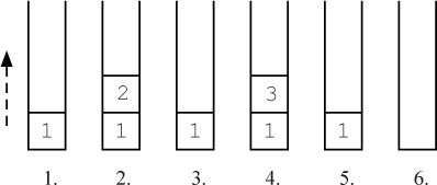
10.8 FURTHER DISCOVERY
The first epigraph at the beginning of this chapter is from the first page of Benoît Mandelbrot’s The Fractal Geometry of Nature [31]. The second is from Shakespeare’s Hamlet, Act II, Scene II.
Aristid Lindenmayer’s work was described in a now freely available book titled, The Algorithmic Beauty of Plants [43], published in 1990.
10.9 PROJECTS
*Project 10.1 Lindenmayer’s beautiful plants
For this project, we assume you have read Section 10.6.
Aristid Lindenmayer was specifically interested in modeling the branching behavior of plants. To accomplish this, we need to introduce two more symbols: [ and ]. For example, consider the following L-system:
Axiom: |
|
Productions: |
|
Angle: |
30 degrees |
These two new symbols involve the use of a simple data structure called a stack. A stack is simply a list in which we only append to and delete from one end. The append operation is called a push and the delete operation is called a pop (hence the name of the list pop method). For example, consider the following sequence of operations on a hypothetical stack object named stack, visualized in Figure 10.20.
stack.push(1)stack.push(2)x = stack.pop()stack.push(3)y = stack.pop()z = stack.pop()
Although we implement a stack as a restricted list, it is usually visualized as a vertical stack of items in which we always push and pop items from the top. The result of the first push operation above results in the leftmost picture in Figure 10.20. After the second push operation, we have two numbers on the stack, with the second number on top of the first, as in the second picture in Figure 10.20. The third operation, a pop, removes the top item, which is then assigned to the variable name x. The fourth operation pushes the value 3 on the top of the stack. The fifth operation pops this value and assigns it to the variable name y. Finally, the bottom value is popped and assigned to the variable name z. The final values of x, y, and z are 2, 3, and 1, respectively.
In Python, we can represent the stack as an initially empty list, implement the push operation as an append and implement the pop operation as a pop with no arguments (which defaults to deleting the last item in the list). So the equivalent sequence of Python statements is:
stack = [ ]       # empty stack; stack is now [ ]
stack.append(1)   # push 1;      stack is now [1]
stack.append(2)   # push 2;      stack is now [1, 2]
x = stack.pop()   # x is now 2;  stack is now [1]
stack.append(3)   # push 3;      stack is now [1, 3]
y = stack.pop()   # y is now 3;  stack is now [1]
z = stack.pop()   # z is now 1;  stack is now [ ]
In a Lindenmayer system, the [ symbol represents a push operation and the ] symbol represents a pop operation. More specifically,
[means “push the turtle’s current position and heading on a stack,” and]means “pop a position and heading from the stack and set the turtle’s current position and heading to these values.”
Let’s now return to the Lindenmayer system above. Applying the productions of this Lindenmayer system twice results in the following string.
X ⇒ F[-X]+X ⇒ FF[-F[-X]+X]+F[-X]+X
The X symbols are used only in the derivation process and do not have any meaning for turtle graphics, so we simply skip them when we are drawing. So the string FF[-F[-X]+X]+F[-X]+X represents the simple “tree” below. On the left is a drawing of the tree; on the right is a schematic we will use to explain how it was drawn.

The turtle starts at the origin, marked O, with a heading of 90 degrees (north). The first two F symbols move the turtle forward from the origin to point a and then point b. The next symbol, [, means that we push the current position and heading (b, 90 degrees) on the stack.
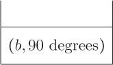
The next two symbols, -F, turn the turtle left 30 degrees (to a heading of 120 degrees) and move it forward, to point c. The next symbol is another [, which pushes the current position and heading, (c, 120 degrees), on the stack. So now the stack contains two items—(b, 90 degrees) and (c, 120 degrees)—with the last item on top.
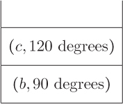
The next three symbols, -X], turn the turtle left another 30 degrees (to a heading of 150 degrees), but then restore its heading to 120 degrees by popping (c, 120 degrees) from the stack.

The next three symbols, +X], turn the turtle 30 degrees to the right (to a heading of 90 degrees), but then pop (b, 90 degrees) from the stack, moving the turtle back to point b, heading north.
![]()
(So, in effect, the previous six symbols, [-X]+X did nothing.) The next two symbols, +F, turn the turtle 30 degrees to the right (to a heading of 60 degrees) and move it forward to point d. Similar to before, the last six symbols, [-X]+X, while pushing states onto the stack, have no visible effect.
Continued applications of the productions in the L-system above will produce strings that draw the same sequence of trees that we created in Section 10.1. More involved L-systems will produce much more interesting trees. For example, the following two L-systems produce the trees in Figure 10.21.
Axiom: |
|
Axiom: |
|
Productions: |
|
Production: |
|
|
|
Angle: |
22.5 degrees |
Angle: |
25 degrees |
|
|

Figure 10.21 Two trees from The Algorithmic Beauty of Plants ([43], p. 25).
Question 10.1.1 Using an angle of 20 degrees, draw the figure corresponding to the string
FF-[-F+F+F]+[+F-F-F]
(Graph paper might make this easier.)
Question 10.1.2 Using an angle of 30 degrees, draw the figure corresponding to the string
FF-[[FF+F]+FF+F]+FF[+FFFF+F]-FF+F
Part 1: Draw L-systems with a stack
If you have not completed Exercises 10.6.1 and 10.6.3, do that first. Then incorporate these functions, with the derive from Section 10.6, into a complete program. Your main function should call the lsystem function to draw a particular L-system.
Next, augment the drawLSystem function from Exercise 10.6.1 so that it correctly draws L-system strings containing the [ and ] characters. Do this by incorporating a single stack into your function, as we described above. Test your function with the three tree-like L-systems above.
Part 2: Draw L-systems recursively
The drawLSystem function can be implemented without an explicit stack by using recursion. Think of the drawLSystem function as drawing the figure corresponding to a string situated inside matching square brackets. We will pass the index of the first character after the left square bracket ([) as an additional parameter:
drawLSystem(tortoise, string, startIndex, angle, distance)
The function will return the index of the matching right square bracket (]). (We can pretend that there are imaginary square brackets around the entire string for the initial call of the function, so we initially pass in 0 for startIndex.) The recursive function will iterate over the indices of the characters in string, starting at startIndex. (Use a while loop, for reasons we will see shortly.) When it encounters a non-bracket character, it should do the same thing it did earlier. When the function encounters a left bracket, it will save the turtle’s current position and heading, and then recursively call the function with startIndex assigned to the index of the character after the left bracket. When this recursive call returns, the current index should be set to the index returned by the recursive call, and the function should reset the turtle’s position and heading to the saved values. When it encounters a right bracket, the function will return the index of the right bracket.
For example, the string below would be processed left to right but when the first left bracket is encountered, the function would be called recursively with index 5 passed in for startIndex.

This recursive call will return 26, the index of the corresponding right bracket, and the + symbol at index 27 would be the next character processed in the loop. The function will later make two more recursive calls, marked with the two additional braces above.
Using this description, rewrite drawLSystem as a recursive function that does not use an explicit stack. Test your recursive function with the same tree-like L-systems, as above.
Question 10.1.3 Why can the stack used in Part 1 be replaced by recursion in Part 2? Referring back to Figures 10.11 and 10.12, how are recursive function calls similar to pushing and popping from a stack?
Question 10.1.4 Use your program to draw the following additional Lindenmayer systems. For each one, set distance = 5, position = (0, –300), heading = 90, and depth = 6.
Axiom: |
|
Productions: |
|
Angle: |
30 degrees |
Axiom: |
|
Productions: |
|
Angle: |
25.7 degrees |
Project 10.2 Gerrymandering
This project assumes that you have read Section 9.3 and the part of Section 10.5 on depth-first search.
U.S. states are divided into electoral districts that each elect one person to the U.S. House of Representatives. Each district is supposed to occupy a contiguous area and represent an approximately equal number of residents. Ideally, it is also compact, i.e., not spread out unnecessarily. More precisely, it should have a relatively small perimeter relative to the area that it covers or, equivalently, enclose a relatively large area for a shape with its perimeter length. A perfect circle is the most compact shape, while an elongated shape, like the one on the right below, is not compact.

These two shapes actually have the same perimeter, but the shape on the right contains only about seven percent of the area of the circle on the left.
In some states, the majority political party has control over periodic redistricting. Often, the majority exploits this power by drawing district lines that favor their chances for re-election, a practice that has come to be known as gerrymandering. These districts often take on bizarre, non-compact shapes.
Several researchers have developed algorithms that redistrict states objectively to optimize various measures of compactness. For example, the image below on the left shows a recent district map for the state of Ohio. The image on the right shows a more compact district map.2

The districts on the right certainly appear to be more compact (less gerrymandered), but how much better are they? In this project, we will write a program that answers this question by determining the compactness of the districts in images like these.
Part 1: Measuring compactness
The compactness of a region can be measured in several ways. We will consider three possibilities:
First, we can measure the mean of the distance between each voter and the centroid of the district. The centroid is the “average point,” computed by averaging all of the x and y values inside the district. We might expect a gerrymandered district to have a higher mean distance than a more compact district. Since we will not actually have information fine enough to compute this value for individual voters, we will compute the average distance between the centroid and each pixel in the image of the district.
Second, we can measure the standard deviation of the distance between each pixel and the centroid of the district. The standard deviation measures the degree of variability from the average. Similar to above, we might expect a gerrymandered district to have higher variability in this distance. The standard deviation of a list of values (in this case, distances) is the square root of the variance. (See Exercise 8.1.10.)
Third, we can compare the area of the district to the area of a (perfectly compact) circle with the same perimeter. In other words, we can define
Intuitively, a circle with a given perimeter encloses the maximum area possible for that perimeter and hence has compactness 1. A gerrymandered shape with the same perimeter encloses far less area, as we saw in the illustration above, and hence has compactness less than 1.
Suppose that we measure a particular district and find that it has area A and perimeter p. To find the value for the denominator of our formula, we need to express the area of a circle, which is normally expressed in terms of the radius r (i.e., πr2), in terms of p instead. To do this, recall that the formula for the perimeter of a circle is p = 2πr. Therefore, r = p/(2π). Substituting this into the standard formula, we find that the area of a circle with perimeter p is
Finally, incorporating this into the formula above, we have

To compute values for the first and second compactness measures, we need a list of the coordinates of all of the pixels in each district. With this list, we can find the centroid of the district, and then compute the mean and standard deviation of the distances from this centroid to the list of coordinates. To compute the third metric, we need to be able to determine the perimeter and area of each district.
Part 2: Measure the districts
We can accomplish all of this by using a variant of depth-first search called a flood fill algorithm. The idea is to start somewhere inside a district and then use DFS to explore the pixels in that district until a pixel with a different color is reached. This is illustrated in Figure 10.22. In this small example, the red and blue squares represent two different districts on a very small map. To explore the red district, we start at some square inside the district, in this case the square marked 0. We then explore outward using a depth-first search. As we did in Section 10.5, we will explore in clockwise order: east, south, west, north. In Figure 10.22(b), we mark the first square as visited by coloring it white and then recursively visit the square to the east, marked 1. After marking square 1 as visited (colored white), the algorithm explores square 2 to the east recursively, as shown in Figure 10.22(c). After marking square 2 as visited, the algorithm backtracks to square 1 because all four neighbors of square 2 are either a different color or have already been visited. From square 1, the algorithm next explores square 3 to the north, as shown in Figure 10.22(d). This process continues until the entire red area has been visited. The numbers indicate the order in which the squares are first visited. As each square is visited for the first time, the algorithm also appends its coordinates to a list (as discussed at the end of Section 10.5). When the algorithm finishes, this list contains the coordinates of all of the squares in the red region.
Based on the dfs function from Section 10.5, implement this flood fill algorithm in the function
measureDistrict(map, x, y, color, points)
The five parameters have the following meanings:
mapis the name of anImageobject (see Section 9.3) containing the district map. The flood fill algorithm will be performed on the pixels in this object rather than on a separate two-dimensional grid. There are several state maps available on the book web site, all of which look similar to the maps of Ohio above.xandyare the coordinates of the pixel from which to begin the depth-first search.coloris the color of the district being measured. This is used to tell whether the current pixel is in the desired region. You may notice that the colors of the pixels in each district are not entirely uniform across the district. (The different shades represent different population densities.) Therefore, the algorithm cannot simply check whether the color of the current pixel is equal tocolor. Rather, it needs to check whether the color of the current pixel is close tocolor. Since colors are represented as three-element tuples, we can treat them as three-dimensional points and use the traditional Euclidean distance formula to determine “closeness:”Start with a distance threshold for closeness of 100, and adjust as needed.
pointswill be a list of coordinates of the pixels that the algorithm visited. When you call the function, initially pass in an empty list. When the function returns, this list should be populated with the coordinates in the district.
Your function should return a tuple containing the total perimeter and total area obtained from a DFS starting at (x, y). The perimeter can be obtained by counting the number of times the algorithm reaches a pixel that is outside of the region (think base case), and the area is the total number of pixels that are visited inside the region. For example, as shown below, the region from Figure 10.22 has perimeter 18 and area 11. The red numbers indicate the order in which the flood fill algorithm will count each border.

Given these measurements, the compactness of this region is
The value of points after calling the function on this example would be
[(3, 1), (3, 2), (3, 3), (2, 2), (2, 1), (2, 0), (3, 0),
 (4, 0), (4, 1), (1, 2), (1, 3)]
The centroid of these points, derived by the averaging the x and y coordinates, is (28/11, 15/11) ≈ (2.54, 1.36). Then the mean distance to the centroid is approximately 1.35 and the standard deviation is approximately 0.54.
Part 3: Compare district maps
To compute the average compactness metrics for a particular map, write a function
compactness(imageName, districts)
that computes the three compactness measurements that we discussed above for the district map with file name imageName. You can find maps for several states on the book web site. The second parameter districts will contain a list of starting coordinates (two-element tuples) for the districts on the map. These are also available on the book web site. Your function should iterate over this list of tuples, and call your measureDistrict function with x and y set to the coordinates in each one.
The function should return a three-element tuple containing the average value, over all of the districts, for each of the three metrics. To make sure your flood fill is working properly, it will also be helpful to display the map (using the show method of the Image class) and update it (using the update method of the Image class) in each iteration. You should see the districts colored white, one by one.
For at least three states, compare the existing district map and the more compact district map, using the three compactness measures. What do you notice?
To drive your program, write a main function that calls the compactness function with a particular map, and then reports the results. As always, think carefully about the design of your program and what additional functions might be helpful.
Technical notes
The images supplied on the book web site have low resolution to keep the depth of the recursive calls in check. As a result, your compactness results will only be a rough approximation. Also, shrinking the image sizes caused some of the boundaries between districts to become “fuzzy.” As a result, you will see some unvisited pixels along these boundaries when the flood fill algorithm is complete.
Depending on your particular Python installation, the depth of recursion necessary to analyze some of these maps may exceed the maximum allowed. To increase the allowed recursion depth, you can call the
sys.setrecursionlimitfunction at the top of your program. For example,import sys
sys.setrecursionlimit(10000)However, set this value carefully. Use the smallest value that works. Setting the maximum recursion depth too high may crash Python on your computer! If you cannot find a value that works on your computer, try shrinking the image file instead (and scaling the starting coordinates appropriately).
Project 10.3 Percolation
This project assumes that you are familiar with two-dimensional grids from Section 9.2 and have read the part of Section 10.5 on depth-first search.
Suppose we have a grid of squares called sites. A site can either be open (white) or blocked (black).

Now imagine that we pour a liquid uniformly over the top of the grid. The liquid will fill the open sites at the top and percolate to connected open sites until the liquid fills all of the open sites that are reachable from an open site at the top. We say that the grid percolates if at least one open site in the bottom row is full at the end. For example, the grid below on the left percolates, while the grid on the right does not.

This system can be used to model a variety of naturally occurring phenomena. Most obviously, it can model a porous rock being saturated with water. Similarly, it can model an oil (or natural gas) field; in this case, the top of the grid represents the oil underground and percolation represents the oil reaching the surface. Percolation systems can also be used to model the flow of current through a network of transistors, whether a material conducts electricity, the spread of disease or forest fires, and even evolution.
We can represent how “porous” a grid is by a vacancy probability, the probability that any particular site is open. For a variety of applications, scientists are interested in knowing the probability that a grid with a particular vacancy probability will percolate. In other words, we would like to know the percolation probability for any vacancy probability p. Despite decades of research, there is no known mathematical solution to this problem. Therefore, we will use a Monte Carlo simulation to estimate it.
Recall from Chapter 5 that a Monte Carlo simulation flips coins (metaphorically speaking) at each step in a computation. For example, to estimate the distance traveled by a random walk, we performed many random walks and took the average final distance from the origin. In this problem, for any given vacancy probability p, we will create many random grids and then test whether they percolate. By computing the number that do percolate divided by the total number of trials, we will estimate the percolation probability for vacancy probability p.
Part 1: Does it percolate?
To decide whether a grid percolates, we can use a depth-first search. Recall from Section 10.5 that the depth-first search algorithm completely explores a space by first exploring as far away as possible from the source. Then it backtracks to follow paths that branch off. To decide whether a given grid percolates, we must do a depth-first search from each of the open sites in the top row. Once this is done, we simply look at whether any site in the bottom row has been visited. If so, the system percolates. Write a function
percolates(grid, draw)
that decides whether a given grid percolates. The second parameter is a Boolean that indicates whether the grid should also be drawn using turtle graphics. There is a skeleton program on the book web site in which the drawing code has already been written. Notice that some of the functions include a Boolean parameter that indicates whether the percolation should be visualized.
Part 2: Find the percolation probability
For any particular vacancy probability p, we can design a Monte Carlo simulation to estimate the percolation probability:
Create a random grid in which, with vacancy probability p, any particular site is open.
Test to see if this grid percolates.
Repeat steps 1 and 2 a large number of times (say, 10,000), keeping track of the number of grids that percolate.
Divide the number that percolate by the total number of trials. This is your estimated percolation probability.
Implement this algorithm with a function
percMonteCarlo(rows, columns, p, trials)
Part 3: When is a grid likely to percolate?
For what vacancy probability does the percolation probability reach at least 1/2? In other words, what must the vacancy probability be for a system to be more likely than not to percolate?
To answer this question, also write a function
percPlot(minP, maxP, stepP, trials)
that plots vacancy probability on the x axis and percolation probability on the y axis for vacancy probabilities minP, minP + stepP, ..., maxP. Each percolation probability should be derived from a Monte Carlo simulation with the given number of trials.
You should discover a phase transition: if the vacancy probability is less than a particular threshold value, the system almost certainly does not percolate; but if the vacancy probability is greater than this threshold value, the system almost certainly does percolate. What is this threshold value?
1http://www.cs.wm.edu/~pkstoc/toh.html
2These figures were produced by an algorithm developed by Brian Olson and retrieved from http://bdistricting.com