2. The Nature of Loads

Search in book...
Toggle Font Controls
Create new playlist

Name your new playlist

Playlist description (optional)
Sign In

Email address

Password

Forgot Password?

or

Continue with Facebook

Continue with Google
Sign Up

Full Name

Email address

Confirm Email Address

Password

or

Continue with Facebook

Continue with Google

The modeling and analysis of a power system depend upon the “load.” What is load? The answer to that question depends upon the type of the analysis that is desired. For example, the steady-state analysis (power-flow study) of an interconnected transmission system will require a different definition of load than that is used in the secondary analysis in a distribution feeder. The problem is that the “load” on a power system is constantly changing. The closer you are to the customer, the more pronounced will be the ever-changing load. There is no such thing as a “steady-state” load. To come to grips with a load, it is first necessary to look at the “load” of an individual customer.

2.1 Definitions

The load that an individual customer or a group of customers presents to the distribution system is constantly changing. Every time a light bulb or an electrical appliance is switched on or off, the load seen by the distribution feeder changes. To describe the changing load, the following terms are defined:

Demand
- Load averaged over a specific period of time
- Load can be kW, kvar, kVA, and A
- Must include the time interval
- Example: The 15-min kW demand is 100 kW
Maximum demand
- Greatest of all demands that occur during a specific time
- Must include demand interval, period, and units
- Example: The 15-min maximum kW demand for the week was 150 kW
Average demand
- The average of the demands over a specified period (day, week, month, etc.)
- Must include demand interval, period, and units
- Example: The 15-min average kW demand for the month was 350 kW
Diversified demand
- Sum of demands imposed by a group of loads over a particular period
- Must include demand interval, period, and units
- Example: The 15-min diversified kW demand in the period between 9:15 and 9:30 was 200 kW
Maximum diversified demand
- Maximum of the sum of the demands imposed by a group of loads over a particular period
- Must include demand interval, period, and units
- Example: The 15-min maximum diversified kW demand for the week was 500 kW
Maximum noncoincident demand
- For a group of loads, the sum of the individual maximum demands without any restriction that they occur at the same time
- Must include demand interval, period, and units
- Example: The maximum noncoincident 15-min kW demand for the week was 700 kW
Demand factor
- Ratio of maximum demand to connected load
Utilization factor
- Ratio of the maximum demand to rated capacity
Load factor
- Ratio of the average demand of any individual customer or a group of customers over a period to the maximum demand over the same period
Diversity factor
- Ratio of the “maximum noncoincident demand” to the “maximum diversified demand”
Load diversity
- Difference between “maximum noncoincident demand” and the “maximum diversified demand”

2.2 Individual Customer Load

Figure 2.1 illustrates how the instantaneous kW load of a customer changes during two 15-min intervals.

2.2.1 Demand

To define the load, the demand curve is broken into equal time intervals. In Figure 2.1, the selected time interval is 15 min. In each interval, the average value of the demand is determined. In Figure 2.1, the straight lines represent the average load in a time interval. The shorter the time interval, the more accurate will be the value of the load. This process is very similar to numerical integration. The average value of the load in an interval is defined as the “15-min kW demand.”

The 24-h 15-min kW demand curve for a customer is shown in Figure 2.2. This curve is developed from a spreadsheet that gives the 15-min kW demand for a period of 24 h.

2.2.2 Maximum Demand

The demand curve shown in Figure 2.2 represents a typical residential customer. Each bar represents the “15-min kW demand.” Note that during the 24-h period, there is a great variation in the demand. This particular customer has three periods in which the kW demand exceeds 6.0 kW. The greatest of these is the “15-min maximum kW demand.” For this customer, the “15-min maximum kW demand” occurs at 13:15 and has a value of 6.18 kW.

images

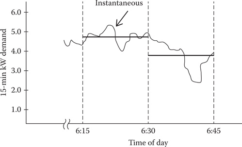
FIGURE 2.1
Customer demand curve.

images

FIGURE 2.2
24-h demand curve for Customer #1.

2.2.3 Average Demand

During the 24-h period, energy (kWh) will be consumed. The energy in kWh used during each 15-min time interval is computed by:

k W h = (15 min kW demand) \cdot \frac{1}{4} \cdot h

$k W h = (15 min kW demand) \cdot \frac{1}{4} \cdot h$ (2.1)

The total energy consumed during the day is then the summation of all of the 15-min interval consumptions. From the spreadsheet, the total energy consumed during the period by Customer #1 is 58.96 kWh. The “15-min average kW demand” is computed by:

k W_{average} = \frac{Total energy}{Hours} = \frac{58.96}{24} = 2.46 kW

$k W_{average} = \frac{Total energy}{Hours} = \frac{58.96}{24} = 2.46 kW$ (2.2)

2.2.4 Load Factor

“Load factor” is a term that is often referred to when describing a load. It is defined as the ratio of the average demand to the maximum demand. In many ways, load factor gives an indication of how well the utility’s facilities are being utilized. From the utility’s standpoint, the optimal load factor would be 1.00, because the system has to be designed to handle the maximum demand. Sometimes, utility companies will encourage industrial customers to improve their load factor. One method of encouragement is to penalize the customer on the electric bill for having a low load factor.

For Customer #1 in Figure 2.2, the load factor is computed to be:

Load factor = \frac{k W_{average}}{k W_{maximum}} = \frac{2.46}{6.18} = 0.40

$Load factor = \frac{k W_{average}}{k W_{maximum}} = \frac{2.46}{6.18} = 0.40$ (2.3)

2.3 Distribution Transformer Loading

A distribution transformer will provide service to one or more customers. Each customer will have a demand curve similar to that shown in Figure 2.2. However, the peaks, valleys, and maximum demands will be different for each customer. Figures 2.3, 2.4, and 2.5 give the demand curves for the three additional customers connected to the same distribution transformer.

The load curves for the four customers show that each customer has a unique loading characteristic. The customers’ individual maximum kW demand occurs at different times of the day. Customer #3 is the only customer who will have a high load factor. A summary of individual loads is given in Table 2.1.

These four customers demonstrate that there is great diversity between their loads.

images

FIGURE 2.3
24-h demand curve for Customer #2.

images

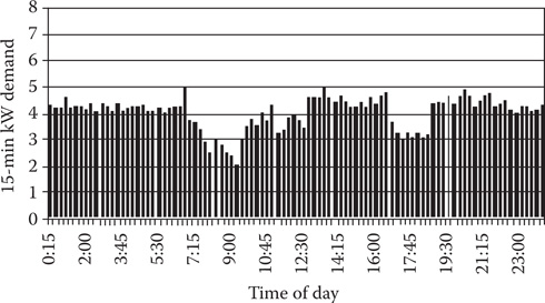
FIGURE 2.4
24-h demand curve for Customer #3.

images

FIGURE 2.5
24-h demand curve for Customer #4.

TABLE 2.1
Individual Customer Load Characteristics

images

2.3.1 Diversified Demand

It is assumed that the same distribution transformer serves the four customers discussed previously. The sum of the four 15 kW demands for each time interval is the “diversified demand” for the group in that time interval, and in this case, the distribution transformer. The 15-min diversified kW demand of the transformer for the day is shown in Figure 2.6. Figure 2.6 shows how the demand curve is beginning to smooth out. There are not as many significant changes as seen by some of the individual customer curves.

2.3.2 Maximum Diversified Demand

The transformer demand curve of Figure 2.6 demonstrates how the combined customer loads begin to smooth out the extreme changes of the individual loads. For the transformer, the 15-min kW demand exceeds 16 kW twice. The greater of these is the “15-min maximum diversified kW demand” of the transformer. It occurs at 17:30 and has a value of 16.16 kW. Note that this maximum demand does not occur at the same time as any one of the individual demands nor is this maximum demand the sum of the individual maximum demands.

images

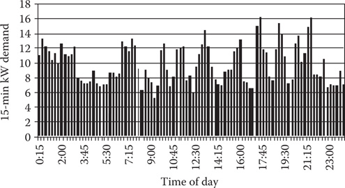
FIGURE 2.6
Transformer diversified demand curve.

images

FIGURE 2.7
Transformer load duration curve.

2.3.3 Load Duration Curve

A “load duration curve” can be developed for the transformer serving the four customers. Sorting the kW demand of the transformer in a descending order develops the load duration curve shown in Figure 2.7.

The load duration curve plots the 15-min kW demand vs. the percent of time the transformer operates at or above the specific kW demand. For example, the load duration curve shows that the transformer operates with a 15-min kW demand of 12 kW or greater 22% of the time. This curve can be used to determine whether or not a transformer needs to be replaced as a result of an overloading condition.

2.3.4 Maximum Noncoincident Demand

The “15-min maximum noncoincident kW demand” for the day is the sum of the individual customer 15-min maximum kW demands. For the transformer in question, the sum of the individual maximums is:

k W_{maximum noncoincident demand} = 6.18 + 6.82 + 4.93 + 7.05 = 24.98 kW

$k W_{maximum noncoincident demand} = 6.18 + 6.82 + 4.93 + 7.05 = 24.98 kW$ (2.4)

2.3.5 Diversity Factor

By definition, diversity factor is the ratio of the maximum noncoincident demand of a group of customers to the maximum diversified demand of the group. With reference to the transformer serving four customers, the diversity factor for the four customers would be:

Diversity factor = \frac{k W_{maximum noncoincident demand}}{k W_{maximum diversified demand}} = \frac{24.98}{16.15} = 1.5458

$Diversity factor = \frac{k W_{maximum noncoincident demand}}{k W_{maximum diversified demand}} = \frac{24.98}{16.15} = 1.5458$ (2.5)

TABLE 2.2
Diversity Factors

images

The idea behind the diversity factor is that when the maximum demands of the customers are known, then the maximum diversified demand of a group of customers can be computed. There will be a different value of the diversity factor for different numbers of customers. The value computed in Equation 2.5 would apply for four customers. If there were five customers, then a load survey would have to be set up to determine the diversity factor for five customers. This process would have to be repeated for all practical number of customers. Table 2.2 is an example of the diversity factors for the number of customers ranging from 1 up to 70. The table was developed from a database that is different from the four customers that have been discussed previously.

A graph of the diversity factors is shown in Figure 2.8.

Note in Table 2.2 and Figure 2.8 that the value of the diversity factor has basically leveled out when the number of customers has reached 70. This is an important observation because it means, at least for the system from which these diversity factors were determined, that the diversity factor will remain constant at 3.20 from 70 or more customers. In other words, as viewed from the substation, the maximum diversified demand of a feeder can be predicted by computing the total noncoincident maximum demand of all of the customers served by the feeder and dividing by 3.2.

2.3.6 Demand Factor

The demand factor can be defined for an individual customer. For example, the 15-min maximum kW demand of Customer #1 was found to be 6.18 kW. To determine the demand factor, the total connected load of the customer needs to be known. The total connected load will be the sum of the ratings of all of the electrical devices at the customer’s location. Assuming that this total comes to 35 kW, the demand factor is computed to be:

Demand factor = \frac{k W_{maximum demand}}{k W_{total connected load}} = \frac{6.18}{35} = 0.1766

$Demand factor = \frac{k W_{maximum demand}}{k W_{total connected load}} = \frac{6.18}{35} = 0.1766$ (2.6)

The demand factor gives an indication of the percentage of electrical devices that are on when the maximum demand occurs. The demand factor can be computed for an individual customer but not for a distribution transformer or the total feeder.

images

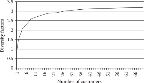
FIGURE 2.8
Diversity factors.

2.3.7 Utilization Factor

The utilization factor gives an indication of how well the capacity of an electrical device is being utilized. For example, the transformer serving the four loads is rated 15 kVA. Using the 16.16 kW maximum diversified demand and assuming a power factor of 0.9, the 15-min maximum kVA demand on the transformer is computed by dividing the 16.16 kW maximum kW demand by the power factor and would be 17.96 kVA. The utilization factor is computed to be:

Utilization factor = \frac{k V A_{maximum demand}}{k V A_{transformer rating}} = \frac{17.96}{15} = 1.197

$Utilization factor = \frac{k V A_{maximum demand}}{k V A_{transformer rating}} = \frac{17.96}{15} = 1.197$ (2.7)

2.3.8 Load Diversity

Load diversity is defined as the difference between the noncoincident maximum demand and the maximum diversified demand. For the transformer in question, the load diversity is computed to be:

Load diversity = 24.97 - 16.16 = 8.81 kW kVA

$Load diversity = 24.97 - 16.16 = 8.81 kW kVA$ (2.8)

2.4 Feeder Load

The load that a feeder serves will display a smoothed-out demand curve as shown in Figure 2.9.

images

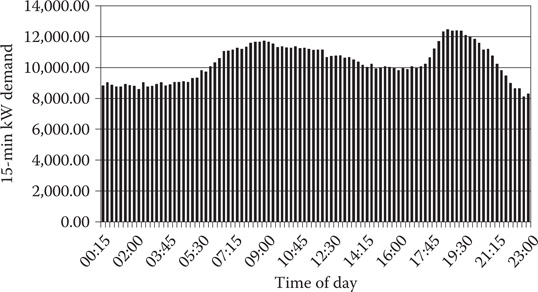
FIGURE 2.9
Feeder demand curve.

The feeder demand curve does not display any of the abrupt changes in demand of an individual customer demand curve or the semi-abrupt changes in the demand curve of a transformer. The simple explanation for this is that with several hundred customers served by the feeder, the odds are good that as one customer is turning off a light bulb, another customer will be turning a light bulb on. The feeder load, therefore, does not experience a jump as would be seen in the individual customer’s demand curve.

2.4.1 Load Allocation

In the analysis of a distribution feeder, “load” data will have to be specified. The data provided will depend upon how detailed the feeder is to be modeled and the availability of customer load data. The most comprehensive model of a feeder will represent every distribution transformer. When this is the case, the load allocated to each transformer needs to be determined.

2.4.1.1 Application of Diversity Factors

The definition of the diversity factor (DF) is the ratio of the maximum noncoincident demand to the maximum diversified demand. A table of diversity factors is shown in Table 2.2. When such a table is available, it is possible to determine the maximum diversified demand of a group of customers such as those served by a distribution transformer. That is, the maximum diversified demand can be computed by:

k W_{maximum diversified demand} = \frac{k W_{maximu noncoincident demand}}{D F_{number of customers}}

$k W_{maximum diversified demand} = \frac{k W_{maximu noncoincident demand}}{D F_{number of customers}}$ (2.9)

This maximum diversified demand becomes the allocated “load” for the transformer.

2.4.1.2 Load Survey

Many times, the maximum demand of individual customers will be known either from metering or from a knowledge of the energy (kWh) consumed by the customer. Some utility companies will perform a load survey of similar customers to determine the relationship between the energy consumption in kWh and the maximum kW demand. Such a load survey requires the installation of a demand meter at each customer’s location. The meter can be the same type as is used to develop the demand curves previously discussed, or it can be a simple meter that only records the maximum demand during the period. At the end of the survey period, the maximum demand vs. kWh for each customer can be plotted on a common graph. Linear regression is used to determine the equation of a straight line that gives the kW demand as a function of kWh. The plot of points for 15 customers along with the resulting equation derived from a linear regression algorithm is shown in Figure 2.10.

images

FIGURE 2.10
kW demand vs. kWh for residential customers.

The straight-line equation derived is:

k W_{maximum demand} = 0.1058 + 0.005014 \cdot kWh

$k W_{maximum demand} = 0.1058 + 0.005014 \cdot kWh$ (2.10)

Knowing the maximum demand for each customer is the first step in developing a table of diversity factors as shown in Table 2.2. The next step is to perform a load survey where the maximum diversified demand of groups of customers is metered. This will involve selecting a series of locations where demand meters can be placed that will record the maximum demand for groups of customers ranging from at least 2–70. At each meter location, the maximum demand of all downstream customers must also be known. With that data, the diversity factor can be computed for the given number of downstream customers.

Example 2.1

A single-phase lateral provides service to three distribution transformers as shown in Figure 2.11.

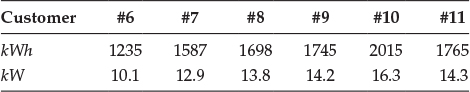
The energy in kWh consumed by each customer during a month is known. A load survey has been conducted for customers in this class, and it has been found that the customer 15-min maximum kW demand is given by the equation:

k W_{demand} = 0.2 + 0.008 \cdot k W h kW

$k W_{demand} = 0.2 + 0.008 \cdot k W h kW$

images

FIGURE 2.11
Single-phase lateral.

The kWh consumed by Customer #1 is 1523 kWh. The 15-min maximum kW demand for Customer #1 is then computed as:

k W_{1} = 0.2 + 0.008 \cdot 1523 = 12.4 kW

$k W_{1} = 0.2 + 0.008 \cdot 1523 = 12.4 kW$

The results of this calculation for the remainder of the customers are summarized in the following table by transformer.

Transformer T1:

images

Transformer T2:

images

Transformer T3:

images

Determine for each transformer the 15-min noncoincident maximum kW demand, and using the Table of Diversity Factors in Table 2.2, determine the 15-min maximum diversified kW demand.

T 1 : \begin{matrix} k W_{maximum noncoincident demand} = 12.4 + 13.4 + 16.1 + 12.9 + 11.8 = 66.6 kW \\ k W_{maximum diversified demand} = \frac{k W_{maximum non-concident demand}}{D F_{5}} = 30.3 kW \end{matrix}

$T 1 : \begin{matrix} k W_{maximum noncoincident demand} = 12.4 + 13.4 + 16.1 + 12.9 + 11.8 = 66.6 kW \\ k W_{maximum diversified demand} = \frac{k W_{maximum non-concident demand}}{D F_{5}} = 30.3 kW \end{matrix}$

T2 : \begin{matrix} k W_{maximum noncoincident demand} = 10.1 + 12.9 + 13.8 + 14.2 + 16.3 + 14.3 = 81.6 kW \\ k W_{maximum diversified demand} = \frac{k W_{maximum non-concident demand}}{D F_{6}} = 35.4 kW \end{matrix}

$T2 : \begin{matrix} k W_{maximum noncoincident demand} = 10.1 + 12.9 + 13.8 + 14.2 + 16.3 + 14.3 = 81.6 kW \\ k W_{maximum diversified demand} = \frac{k W_{maximum non-concident demand}}{D F_{6}} = 35.4 kW \end{matrix}$

T3: \begin{matrix} k W_{maximum noncoincident demand} = 17.0 + 15.0 + 16.7 + 18.3 + 17.3 + 16.1 + 17.0 = 117.4 kW \\ k W_{maximum diversified demand} = \frac{k W_{maximum non-concident demand}}{D F_{7}} = 48.9 kW \end{matrix}

$T3: \begin{matrix} k W_{maximum noncoincident demand} = 17.0 + 15.0 + 16.7 + 18.3 + 17.3 + 16.1 + 17.0 = 117.4 kW \\ k W_{maximum diversified demand} = \frac{k W_{maximum non-concident demand}}{D F_{7}} = 48.9 kW \end{matrix}$

Based upon the 15-min maximum kW diversified demand on each transformer and an assumed power factor of 0.9, the 15-min maximum kVA diversified demand on each transformer would be:

\begin{array}{l} k V A_{T 1-}_{maximum diversified demand} = \frac{30.2}{0.9} = 33.6 kVA \\ k V A_{T 2-}_{maximum diversified demand} = \frac{35.5}{0.9} = 39.4 kVA \\ k V A_{T 3-}_{maximum diversified demand} = \frac{48.9}{0.9} = 54.4 kVA \end{array}

$\begin{array}{l} k V A_{T 1-}_{maximum diversified demand} = \frac{30.2}{0.9} = 33.6 kVA \\ k V A_{T 2-}_{maximum diversified demand} = \frac{35.5}{0.9} = 39.4 kVA \\ k V A_{T 3-}_{maximum diversified demand} = \frac{48.9}{0.9} = 54.4 kVA \end{array}$

The kVA ratings selected for the three transformers would be 25, 37.5, and 50 kVA, respectively. With those selections, only transformer T1 would experience a significant maximum kVA demand greater than its rating (135%).

2. Determine the 15-min noncoincident maximum kW demand and 15-min maximum diversified kW demand for each of the line segments.

Segment N1 to N2: The maximum noncoincident kW demand is the sum of the maximum demands of all 18 customers.

k W_{maximum noncoincident demand} = 66.6 + 81.6 + 117.4 = 265.6 kW

$k W_{maximum noncoincident demand} = 66.6 + 81.6 + 117.4 = 265.6 kW$

The maximum diversified kW demand is computed by using the diversity factor for 18 customers.

k W_{maximum diversified demand} = \frac{265.5}{2.86} = 92.8 kW

$k W_{maximum diversified demand} = \frac{265.5}{2.86} = 92.8 kW$

Segment N2 to N3: This line segment “sees” 13 customers. The noncoincident maximum demand is the sum of customers’ number 6 through 18. The diversity factor for 13 (2.74) is used to compute the maximum diversified kW demand.

\begin{array}{l} k W_{maximum noncoincident demand} = 81.6 + 117.4 = 199.0 kW \\ k W_{maximum diversified demand} = \frac{199.0}{2.74} = 72.6 kW \end{array}

$\begin{array}{l} k W_{maximum noncoincident demand} = 81.6 + 117.4 = 199.0 kW \\ k W_{maximum diversified demand} = \frac{199.0}{2.74} = 72.6 kW \end{array}$

Segment N3 to N4: This line segment “sees” the same noncoincident demand and diversified demand as that of transformer T3.

\begin{array}{l} k W_{maximum noncoincident demand} = 117.4 = 117.4 kW \\ k W_{maximum diversified demand} = \frac{199.0}{2.4} = 48.9 kW \end{array}

$\begin{array}{l} k W_{maximum noncoincident demand} = 117.4 = 117.4 kW \\ k W_{maximum diversified demand} = \frac{199.0}{2.4} = 48.9 kW \end{array}$

Example 2.1 demonstrates that Kirchhoff’s Current Law (KCL) is not obeyed when the maximum diversified demands are used as the “load” flowing through the line segments and through the transformers. For example, at node N1, the maximum diversified demand flowing down the line segment N1–N2 is 92.8 kW and the maximum diversified demand flowing through transformer T1 is 30.3 kW. KCL would then predict that the maximum diversified demand flowing down line segment N2–N3 would be the difference of these or 62.5 kW. However, the calculations for the maximum diversified demand in that segment was computed to be 72.6 kW. The explanation for this is that the maximum diversified demands for the line segments and transformers do not necessarily occur at the same time. At the time that the line segment N2–N3 is experiencing its maximum diversified demand, line segment N1–N2 and transformer T1 are not at their maximum values. All that can be said is that at the time segment that N2–N3 is experiencing its maximum diversified demand, the difference between the actual demand on the line segment N1–N2 and the demand of transformer T1 will be 72.6 kW. There will be an infinite amount of combinations of line flow down N1–N2 and through transformer T1, which will produce the maximum diversified demand of 72.6 kW on line N2–N3.

2.4.1.3 Transformer Load Management

A transformer load management program is used by utilities to determine the loading on distribution transformers based upon a knowledge of the kWh supplied by the transformer during a peak loading month. The program is primarily used to determine when a distribution transformer needs to be changed out owing to a projected overloading condition. The results of the program can also be used to allocate loads to transformers for feeder analysis purposes.

The transformer load management program relates the maximum diversified demand of a distribution transformer to the total kWh supplied by the transformer during a specific month. The usual relationship is the equation of a straight line. Such an equation is determined from a load survey. This type of load survey meters the maximum demand on the transformer in addition to the total energy in kWh of all of the customers connected to the transformer. With the information available from several sample transformers, a curve similar to that shown in Figure 2.10 can be developed, and the constants of the straight-line equation can then be computed. This method has the advantage because the utility will have the kWh consumed by each customer every month in the billing database. As long as the utility knows as to which customers are connected to each transformer, by using the developed equation the maximum diversified demand (allocated load) on each transformer on a feeder can be determined for each billing period.

2.4.1.4 Metered Feeder Maximum Demand

The major disadvantage of allocating load using the diversity factors is that most utilities would not have a table of diversity factors. The process of developing such a table is generally not cost beneficial. The major disadvantage of the transformer load management method is that a database is required that specifies which transformers serve which customers. Again, this database is not always available.

Allocating load based upon the metered readings in the substation requires the least amount of data. Most feeders will have metering in the substation that will, at a minimum, give either the total three-phase maximum diversified kW or kVA demand and/or the maximum current per phase during a month. The kVA ratings of all distribution transformers is always known for a feeder. The metered readings can be allocated to each transformer based upon the transformer rating. An “allocation factor” (AF) can be determined based upon the metered three-phase kW or kVA demand and the total connected distribution transformer kVA.

A F = \frac{k V A_{metered demand}}{k V A_{total kVA rating}}

$A F = \frac{k V A_{metered demand}}{k V A_{total kVA rating}}$ (2.11)

where kVA_{total kVA rating} = Sum of the kVA ratings of all distribution transformers.

The allocated load per transformer is then determined by:

k V A_{transformer demand} = A F \cdot k V A_{transformer rating}

$k V A_{transformer demand} = A F \cdot k V A_{transformer rating}$ (2.12)

The transformer demand will be either kW or kVA depending upon the metered quantity.

When the kW or kVA is metered by phase, the load can be allocated by phase, where it will be necessary to know the phasing of each distribution transformer.

When the maximum current per phase is metered, the load allocated to each distribution transformer can be done by assuming nominal voltage at the substation and then computing the resulting kVA. The load allocation will now follow the same procedure as outlined earlier.

If there is no metered information on the reactive power or power factor of the feeder, a power factor will have to be assumed for each transformer load.

Modern substations will have microprocessor-based metering that will provide kW, kvar, kVA, power factor, and current per phase. With this data, the reactive power can also be allocated. Because the metered data at the substation will include losses, an iterative process will have to be followed, so that the allocated load plus losses will equal the metered readings.

Example 2.2

Assume that the metered maximum diversified kW demand for the system of Example 2.1 is 92.9 kW. Allocate this load according to the kVA ratings of the three transformers.

k V A_{total} = 25 + 37.5 + 50 = 112.5

$k V A_{total} = 25 + 37.5 + 50 = 112.5$

A F = \frac{92.9}{112.5} = 0.8258 kW/kVA

$A F = \frac{92.9}{112.5} = 0.8258 kW/kVA$

The allocated kW for each transformer becomes:

T1: k W_{1} = 0.8258 \cdot 25 = 20.64 kW

$T1: k W_{1} = 0.8258 \cdot 25 = 20.64 kW$

T2: k W_{2} = 0.8258 \cdot 37.5 = 30.97 kW

$T2: k W_{2} = 0.8258 \cdot 37.5 = 30.97 kW$

T3: k W_{3} = 0.8258 \cdot 50 = 41.29 kW

$T3: k W_{3} = 0.8258 \cdot 50 = 41.29 kW$

2.4.1.5 What Method to Use?

The following four different methods have been presented for allocating load to distribution transformers:

Application of diversity factors
Load survey
Transformer load management
Metered feeder maximum demand

The method to be used depends upon the purpose of the analysis. If the purpose of the analysis is to determine as closely as possible the maximum demand on a distribution transformer, then either the diversity factor or the transformer load management method can be used. Neither of these methods should be employed when the analysis of the total feeder is to be performed. The problem is that using either of those methods will result in a much larger maximum diversified demand at the substation than that actually exists. When the total feeder is to be analyzed, the only method that gives good results is that of allocating load based upon the kVA ratings of the transformers.

2.4.2 Voltage Drop Calculations Using Allocated Loads

The voltage drops down line segments and through distribution transformers are of interest to the distribution engineer. Four different methods of allocating loads have been presented. The various voltage drops can be computed using the loads allocated by the three methods. For these studies, it is assumed that the allocated loads will be modeled as constant real power and reactive power.

2.4.2.1 Application of Diversity Factors

The loads allocated to a line segment or a distribution transformer using diversity factors are a function of the total number of customers “downstream” from the line segment or distribution transformer. The application of the diversity factors was demonstrated in Example 2.1. With a knowledge of the allocated loads flowing in the line segments and through the transformers and the impedances, the voltage drops can be computed. The assumption is that the allocated loads will be constant real power and reactive power. To avoid an iterative solution, the voltage at the source end is assumed and the voltage drops are calculated from that point to the last transformer. Example 2.3 demonstrates how the method of load allocation using diversity factors is applied. The same system and allocated loads from Example 2.1 are used in Example 2.3.

Example 2.3

For the system in Example 2.1, assume the voltage at N1 is 2400 V, and compute the secondary voltages on the three transformers using the diversity factors.

The system in Example 2.1 including segment distances is shown in Figure 2.12.

Assume that the power factor of the loads is 0.9 lagging.

The impedance of the lines are: z = 0.3 + j0.6 Ω/mile

images

FIGURE 2.12
Single-phase lateral with distances.

The ratings of the transformers are:

T1: 25 kVA, 2400–240 V, Z = 1.8/40

T2: 37.5 kVA, 2400–240 V, Z = 1.9/45

T3: 50 kVA, 2400–240 V, Z = 2.0/50

From Example 2.1, the maximum diversified kW demands were computed. Using the 0.9 lagging power factor, the maximum diversified kW and kVA demands for the line segments and transformers are:

Segment N1–N2: P₁₂ = 92.9 kW S₁₂ = 92.9 + j45.0 kVA

Segment N2–N3: P₂₃ = 72.6 kW S₂₃ = 72.6 + j35.2 kVA

Segment N3–N4: P₃₄ = 49.0 kW S₃₄ = 49.0 + j23.7 kVA

Transformer T1: P_T1 = 30.3 kW S_T1 = 30.3 + j14.7 kVA

Transformer T2: P_T2 = 35.5 kW S_T2 = 35.5 + j17.2 kVA

Transformer T3: P_T3 = 49.0 kW S_T3 = 49.0 + j23.7 kVA

Convert transformer impedances to ohms referred to the high-voltage side.

T1: Z_{{base}_{1}} = \frac{k V^{2} \cdot 1000}{k V A_{1}} = \frac{{2.4}^{2} \cdot 1000}{25} = 230.4 Ω

$T1: Z_{{base}_{1}} = \frac{k V^{2} \cdot 1000}{k V A_{1}} = \frac{{2.4}^{2} \cdot 1000}{25} = 230.4 Ω$

Z_{T 1} = (0.018 \underset{___}{/ 40}) \cdot 230.4 = 3.18 + j 2.67 Ω

$Z_{T 1} = (0.018 \underset{___}{/ 40}) \cdot 230.4 = 3.18 + j 2.67 Ω$

T2: Z_{{base}_{2}} = \frac{k V^{2} \cdot 1000}{k V A_{2}} = \frac{{2.4}^{2} \cdot 1000}{37.5} = 153.6 Ω

$T2: Z_{{base}_{2}} = \frac{k V^{2} \cdot 1000}{k V A_{2}} = \frac{{2.4}^{2} \cdot 1000}{37.5} = 153.6 Ω$

Z_{T 2} = (0.019 \underset{___}{/ 45}) \cdot 153.6 = 2.06 + j 2.06 Ω

$Z_{T 2} = (0.019 \underset{___}{/ 45}) \cdot 153.6 = 2.06 + j 2.06 Ω$

T3: Z_{{base}_{3}} = \frac{k V^{2} \cdot 1000}{k V A_{3}} = \frac{{2.4}^{2} \cdot 1000}{50} = 115.2 Ω

$T3: Z_{{base}_{3}} = \frac{k V^{2} \cdot 1000}{k V A_{3}} = \frac{{2.4}^{2} \cdot 1000}{50} = 115.2 Ω$

Z_{T 3} = (0.02 \underset{___}{/ 50}) \cdot 115.2 = 1.48 + j 1.77 Ω

$Z_{T 3} = (0.02 \underset{___}{/ 50}) \cdot 115.2 = 1.48 + j 1.77 Ω$

Compute the line impedances:

N 1 - N 2 : Z_{12} = (0.3 + j 0.6) \cdot \frac{5000}{5280} = 0.2841 + j 0.5682 Ω

$N 1 - N 2 : Z_{12} = (0.3 + j 0.6) \cdot \frac{5000}{5280} = 0.2841 + j 0.5682 Ω$

N 2 - N 3 : Z_{23} = (0.3 + j 0.6) \cdot \frac{500}{5280} = 0.0284 + j 0.0568 Ω

$N 2 - N 3 : Z_{23} = (0.3 + j 0.6) \cdot \frac{500}{5280} = 0.0284 + j 0.0568 Ω$

N 3 - N 4 : Z_{34} = (0.3 + j 0.6) \cdot \frac{750}{5280} = 0.0426 + j 0.0852 Ω

$N 3 - N 4 : Z_{34} = (0.3 + j 0.6) \cdot \frac{750}{5280} = 0.0426 + j 0.0852 Ω$

Calculate the current flowing in segment N1–N2:

I_{12} = {(\frac{k W + j k v a r}{k V})}^{*} = {(\frac{92.9 + j 45.0}{2.4 \underset{__}{/ 0}})}^{*} = 43.0 \underset{_______}{/ - 25.84} A

$I_{12} = {(\frac{k W + j k v a r}{k V})}^{*} = {(\frac{92.9 + j 45.0}{2.4 \underset{__}{/ 0}})}^{*} = 43.0 \underset{_______}{/ - 25.84} A$

Calculate the voltage at N2:

V_{2} = V_{1} - Z_{12} \cdot I_{12}

$V_{2} = V_{1} - Z_{12} \cdot I_{12}$

V_{2} = 2400 \underset{__}{/ 0} - (0.2841 + j 0.5682) \cdot 43.0 \underset{_______}{/ - 25.84} = 2378.4 \underset{_____}{/ - 0.4} V

$V_{2} = 2400 \underset{__}{/ 0} - (0.2841 + j 0.5682) \cdot 43.0 \underset{_______}{/ - 25.84} = 2378.4 \underset{_____}{/ - 0.4} V$

Calculate the current flowing into T1:

I_{T 1} = {(\frac{k W + j k v a r}{k V})}^{*} = {(\frac{30.3 + j 14.7}{2.378 \underset{_____}{/ - 0.4}})}^{*} = 14.16 \underset{______}{/ - 26.24} A

$I_{T 1} = {(\frac{k W + j k v a r}{k V})}^{*} = {(\frac{30.3 + j 14.7}{2.378 \underset{_____}{/ - 0.4}})}^{*} = 14.16 \underset{______}{/ - 26.24} A$

Calculate the secondary voltage referred to the high side:

V_{T 1} = V_{2} - Z_{T 2} \cdot I_{T 2}

$V_{T 1} = V_{2} - Z_{T 2} \cdot I_{T 2}$

V_{T 1} = 2378.4 \underset{_____}{/ - 0.4} - (3.18 + j 2.67) \cdot 14.16 \underset{______}{/ - 26.24} = 2321.5 \underset{_____}{/ - 0.8} V

$V_{T 1} = 2378.4 \underset{_____}{/ - 0.4} - (3.18 + j 2.67) \cdot 14.16 \underset{______}{/ - 26.24} = 2321.5 \underset{_____}{/ - 0.8} V$

Compute the secondary voltage by dividing by the turns ratio of 10:

V_{low}_{_{T 1}} = \frac{2321.5 \underset{_____}{/ - 0.8}}{10} = 232.15 \underset{_____}{/ - 0.8} V

$V_{low}_{_{T 1}} = \frac{2321.5 \underset{_____}{/ - 0.8}}{10} = 232.15 \underset{_____}{/ - 0.8} V$

Calculate the current flowing in line section N2–N3:

I_{23} = {(\frac{k W + j k v a r}{k V})}^{*} = {(\frac{72.6 + j 35.2}{2.378 \underset{_____}{/ - 0.4}})}^{*} = 33.9 \underset{_______}{/ - 26.24} A

$I_{23} = {(\frac{k W + j k v a r}{k V})}^{*} = {(\frac{72.6 + j 35.2}{2.378 \underset{_____}{/ - 0.4}})}^{*} = 33.9 \underset{_______}{/ - 26.24} A$

Calculate the voltage at N3:

V_{3} = V_{2} - Z_{23} \cdot I_{23}

$V_{3} = V_{2} - Z_{23} \cdot I_{23}$

V_{3} = 2378.4 \underset{_____}{/ - 0.4} - (0.0284 + j 0.0568) \cdot 33.9 \underset{_______}{/ - 26.24} = 2376.7 \underset{_____}{/ - 0.4} V

$V_{3} = 2378.4 \underset{_____}{/ - 0.4} - (0.0284 + j 0.0568) \cdot 33.9 \underset{_______}{/ - 26.24} = 2376.7 \underset{_____}{/ - 0.4} V$

Calculate the current flowing into T2:

_{T 2} = {(\frac{k W + j k v a r}{k V})}^{*} = {(\frac{35.5 + j 17.2}{2.3767 \underset{_____}{/ - 0.4}})}^{*} = 16.58 \underset{_______}{/ - 26.27} A

$_{T 2} = {(\frac{k W + j k v a r}{k V})}^{*} = {(\frac{35.5 + j 17.2}{2.3767 \underset{_____}{/ - 0.4}})}^{*} = 16.58 \underset{_______}{/ - 26.27} A$

Calculate the secondary voltage referred to the high side:

V_{T 2} = V_{3} - Z_{T 2} \cdot I_{T 2}

$V_{T 2} = V_{3} - Z_{T 2} \cdot I_{T 2}$

V_{T 2} = 2376.7 \underset{_____}{/ - 0.4} - (2.06 + j 2.06) \cdot 16.58 \underset{_______}{/ - 26.27} = 2331.1 \underset{_____}{/ - 0.8} V

$V_{T 2} = 2376.7 \underset{_____}{/ - 0.4} - (2.06 + j 2.06) \cdot 16.58 \underset{_______}{/ - 26.27} = 2331.1 \underset{_____}{/ - 0.8} V$

Compute the secondary voltage by dividing by the turns ratio of 10:

V_{low}_{_{T 2}} = \frac{2331.1 \underset{_____}{/ - 0.8}}{10} = 233.1 \underset{_____}{/ - 0.8} V

$V_{low}_{_{T 2}} = \frac{2331.1 \underset{_____}{/ - 0.8}}{10} = 233.1 \underset{_____}{/ - 0.8} V$

Calculate the current flowing in line section N3–N4:

I_{34} = {(\frac{k W + j k v a r}{k V})}^{*} = {(\frac{49.0 + j 23.7}{2.3767 \underset{_____}{/ - 0.4}})}^{*} = 22.9 \underset{_______}{/ - 26.27} A

$I_{34} = {(\frac{k W + j k v a r}{k V})}^{*} = {(\frac{49.0 + j 23.7}{2.3767 \underset{_____}{/ - 0.4}})}^{*} = 22.9 \underset{_______}{/ - 26.27} A$

Calculate the voltage at N4:

V_{4} = V_{3} - Z_{34} \cdot I_{34}

$V_{4} = V_{3} - Z_{34} \cdot I_{34}$

V_{4} = 2376.7 \underset{_____}{/ - 0.4} - (0.0426 + 0.0852) \cdot 22.9 \underset{_______}{/ - 26.27} = 2375.0 \underset{_____}{/ - 0.5} V

$V_{4} = 2376.7 \underset{_____}{/ - 0.4} - (0.0426 + 0.0852) \cdot 22.9 \underset{_______}{/ - 26.27} = 2375.0 \underset{_____}{/ - 0.5} V$

The current flowing into T3 is the same as the current from N3 to N4:

I_{T 3} = 22.91 \underset{_______}{/ - 26.30} A

$I_{T 3} = 22.91 \underset{_______}{/ - 26.30} A$

Calculate the secondary voltage referred to the high side:

V_{T 3} = V_{4} - Z_{T 3} \cdot I_{T 3}

$V_{T 3} = V_{4} - Z_{T 3} \cdot I_{T 3}$

V_{T 3} = 2375.0 \underset{_____}{/ - 0.5} - (1.48 + j 1.77) \cdot 22.9 \underset{_______}{/ - 26.27} = 2326.9 \underset{_____}{/ - 1.0} V

$V_{T 3} = 2375.0 \underset{_____}{/ - 0.5} - (1.48 + j 1.77) \cdot 22.9 \underset{_______}{/ - 26.27} = 2326.9 \underset{_____}{/ - 1.0} V$

Compute the secondary voltage by dividing by the turns ratio of 10:

V low_{_{T 3}} = \frac{2326.9 \underset{_____}{/ - 1.0}}{10} = 232.7 \underset{_____}{/ - 1.0} V

$V low_{_{T 3}} = \frac{2326.9 \underset{_____}{/ - 1.0}}{10} = 232.7 \underset{_____}{/ - 1.0} V$

Calculate the percent voltage drop to the secondary of transformer T3. Use the secondary voltage referred to the high side:

V_{drop} = \frac{| V_{1} | - | V_{T 3} |}{| V_{1} |} \cdot 100 = \frac{2400 - 2326.11}{2400} \cdot 100 = 3.0789 %

$V_{drop} = \frac{| V_{1} | - | V_{T 3} |}{| V_{1} |} \cdot 100 = \frac{2400 - 2326.11}{2400} \cdot 100 = 3.0789 %$

2.4.2.2 Load Allocation Based upon Transformer Ratings

When only the ratings of the distribution transformers are known, the feeder can be allocated based upon the metered demand and the transformer kVA ratings. This method was discussed in Section 2.3.3. Example 2.4 demonstrates this method.

Example 2.4

For the system in Example 2.1, assume the voltage at N1 is 2400 V, and compute the secondary voltages on the three transformers allocating the loads based upon the transformer ratings. Assume that the metered kW demand at N1 is 92.9 kW. The impedances of the line segments and transformers are the same as in Example 2.3.Assume the load power factor is 0.9 lagging, and compute the kVA demand at N1 from the metered demand:

S_{12} = \frac{92.9}{0.9} \underset{________}{/ \cos^{- 1} (0.9)} = 92.9 + j 45.0 = 103.2 \underset{_____}{/ 25.84} kVA

$S_{12} = \frac{92.9}{0.9} \underset{________}{/ \cos^{- 1} (0.9)} = 92.9 + j 45.0 = 103.2 \underset{_____}{/ 25.84} kVA$

Calculate the allocation factor:

A F = \frac{103.2 \underset{_____}{/ 25.84}}{25 + 37.5 + 50} = 0.9175 \underset{_____}{/ 25.84}

$A F = \frac{103.2 \underset{_____}{/ 25.84}}{25 + 37.5 + 50} = 0.9175 \underset{_____}{/ 25.84}$

Allocate the loads to each transformer:

S_{T 1} = A F \cdot k V A_{T 1} = (0.9175 \underset{_____}{/ 25.84}) \cdot 25 = 20.6 + j 10.0 kVA

$S_{T 1} = A F \cdot k V A_{T 1} = (0.9175 \underset{_____}{/ 25.84}) \cdot 25 = 20.6 + j 10.0 kVA$

S_{T 2} = A F \cdot k V A_{T 2} = (0.9175 \underset{_____}{/ 25.84}) \cdot 37.5 = 31.0 + j 15.0 kVA

$S_{T 2} = A F \cdot k V A_{T 2} = (0.9175 \underset{_____}{/ 25.84}) \cdot 37.5 = 31.0 + j 15.0 kVA$

S_{T 3} = A F \cdot k V A_{T 3} = (0.9175 \underset{_____}{/ 25.84}) \cdot 50 = 41.3 + j 20.0 kVA

$S_{T 3} = A F \cdot k V A_{T 3} = (0.9175 \underset{_____}{/ 25.84}) \cdot 50 = 41.3 + j 20.0 kVA$

Calculate the line flows:

S_{1} = S_{T 1} + S_{T 2} + S_{T 3} = 92.9 + j 45.0 kVA

$S_{1} = S_{T 1} + S_{T 2} + S_{T 3} = 92.9 + j 45.0 kVA$

S_{23} = S_{T 2} + S_{T 3} = 72.3 + j 35 kVA

$S_{23} = S_{T 2} + S_{T 3} = 72.3 + j 35 kVA$

S_{34} = S_{T 3} = 41.3 + j 20.0 kVA

$S_{34} = S_{T 3} = 41.3 + j 20.0 kVA$

Using these values of line flows and flows into transformers, the procedure for computing the transformer secondary voltages is exactly the same as in Example 2.3. When this procedure is followed, the node and secondary transformer voltages are:

V_{2} = 2378.1 \underset{_____}{/ - 0.4} V, V low_{_{T 1}} = 234.0 \underset{_____}{/ - 0.6} V

$V_{2} = 2378.1 \underset{_____}{/ - 0.4} V, V low_{_{T 1}} = 234.0 \underset{_____}{/ - 0.6} V$

V_{3} = 2376.4 \underset{_____}{/ - 0.4} V, V low_{_{T 2}} = 233.7 \underset{_____}{/ - 0.8} V

$V_{3} = 2376.4 \underset{_____}{/ - 0.4} V, V low_{_{T 2}} = 233.7 \underset{_____}{/ - 0.8} V$

V_{4} = 2374.9 \underset{_____}{/ - 0.5} V, V low_{_{T 3}} = 233.5 \underset{_____}{/ - 0.9} V

$V_{4} = 2374.9 \underset{_____}{/ - 0.5} V, V low_{_{T 3}} = 233.5 \underset{_____}{/ - 0.9} V$

The percent voltage drop for this case is:

V_{drop} = \frac{| V_{1} | - | V_{T 3} |}{| V_{1} |} \cdot 100 = \frac{2400 - 2334.8}{2400} \cdot 100 = 2.7179

$V_{drop} = \frac{| V_{1} | - | V_{T 3} |}{| V_{1} |} \cdot 100 = \frac{2400 - 2334.8}{2400} \cdot 100 = 2.7179$

2.5 Summary

This chapter has demonstrated the nature of the loads on a distribution feeder. There is a great diversity between individual customer demands, but as the demand is monitored on line segments working back toward the substation, the effect of the diversity between demands becomes very light. It was shown that the effect of diversity between customer demands must be taken into account when the demand on a distribution transformer is computed. The effect of diversity for short laterals can be taken into account in determining the maximum flow on the lateral. For the diversity factors of Table 2.2, it was shown that when the number of customers exceeds 70, the effect of diversity has pretty much disappeared. This is evidenced by the fact that the diversity factor has become almost constant as the number of customers approached 70. It must be understood that the number 70 will apply only to the diversity factors of Table 2.2. If a utility is going to use diversity factors, then that utility must perform a comprehensive load survey to develop the table of diversity factors that apply to that particular system.

Examples 2.3 and 2.4 show that the final node and transformer voltages are approximately the same. There is very little difference between the voltages when the loads were allocated using the diversity factors and when the loads were allocated based upon the transformer kVA ratings.

Problems

2.1 Shown below are the 15-min kW demands for four customers between the hours of 17:00 and 21:00. A 25-kVA single-phase transformer serves the four customers.

a. For each of the customers, determine:
1. Maximum 15-min kW demand
2. Average 15-min kW demand
3. Total kWh usage in the time period
4. Load factor
b. For the 25-kVA transformer, determine:
1. Maximum 15-min diversified demand
2. Maximum 15-min noncoincident demand
3. Utilization factor (assume unity power factor)
4. Diversity factor
5. Load diversity
c. Plot the load duration curve for the transformer

images

FIGURE 2.13
System for Problem 2.2.

2.2 Two transformers each serving four customers are shown in Figure 2.13:

The following table gives the time interval and kVA demand of the four customer demands during the peak load period of the year. Assume a power factor of 0.9 lagging.

images

a. For each transformer, determine the following:
1. 30-min maximum kVA demand
2. Noncoincident maximum kVA demand
3. Load factor
4. Diversity factor
5. Suggested transformer rating (50, 75, 100, 167)
6. Utilization factor
7. Energy (kWh) during the 4 h period
b. Determine the maximum diversified 30-min kVA demand at the “Tap”

2.3 Two single-phase transformers serving 12 customers are shown in Figure 2.14.

images

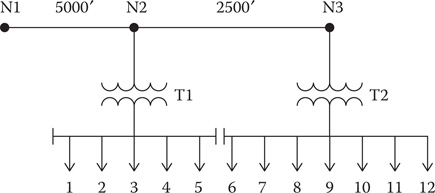
FIGURE 2.14
Circuit for Problem 2.3.

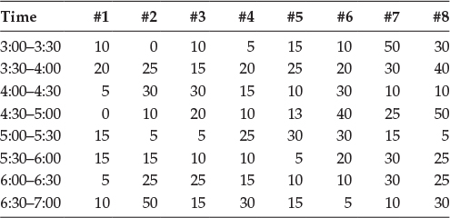
The 15-min kW demands for the 12 customers between the hours of 5:00 pm and 9:00 pm are given in the following tables. Assume a load power factor of 0.95 lagging. The impedance of the lines are z = 0.306 + j0.6272 Ω/mile. The voltage at node N1 is 2500/0 V.

Transformer ratings:

a. Determine the maximum kW demand for each customer
b. Determine the average kW demand for each customer
c. Determine the kWH consumed by each customer in this time period
d. Determine the load factor for each customer
e. Determine the maximum diversified demand for each transformer
f. Determine the maximum noncoincident demand for each transformer
g. Determine the utilization factor (assume 1.0 power factor) for each transformer
h. Determine the diversity factor of the load for each transformer
i. Determine the maximum diversified demand at Node N1
j. Compute the secondary voltage for each transformer taking diversity into account

Transformer #1—25 kVA

images

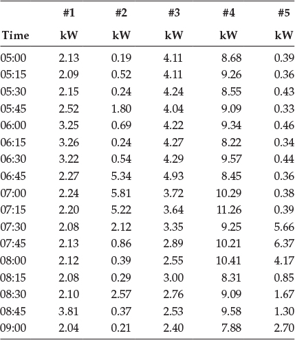
Transformer #2—37.5 kVA

images

2.4 On a different day, the metered 15-min kW demand at node N1 for the system of Problem 2.3 is 72.43 kW. Assume a power factor of 0.95 lagging. Allocate the metered demand to each transformer based upon the transformer kVA rating. Assume the loads are constant current, and compute the secondary voltage for each transformer.

2.5 A single-phase lateral serves four transformers as shown in Figure 2.15.

Assume that each customer’s maximum demand is 15.5 kW + j7.5 kvar. The impedance of the single-phase lateral is z = 0.4421 + j0.3213 Ω/1000 ft. The four transformers are rated as:

T1 and T2: 37.5 kVA, 2400–240 V, Z = 0.01 + j0.03 per unit
T3 and T4: 50 kVA, 2400–240 V, Z = 0.015 + j0.035 per unit

images

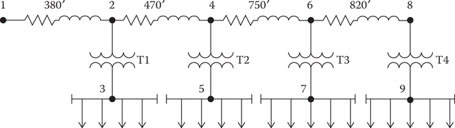
FIGURE 2.15
System for Problem 2.5.

Use the diversity factors found in Table 2.2 and determine:

The 15-min maximum diversified kW and kvar demands on each transformer
The 15-min maximum diversified kW and kvar demands for each line section
If the voltage at Node 1 is 2600/0 V, determine the voltage at nodes 2, 3, 4, 5, 6, 7, 8, and 9. In calculating the voltages, take into account diversity using the answers from (1) and (b) above.
Use the 15-min maximum diversified demands at the lateral tap (section 1–2) from part (b). Divide these maximum demands by 18 (number of customers), and assign that as the “instantaneous load” for each customer. Now calculate the voltages at all of the nodes listed in part (c) using the instantaneous loads.
Repeat part (d) above except assuming that the loads are “constant current”. To do this, take the current flowing from node 1 to node 2 from part (d) and divide by 18 (number of customers) and assign that as the “instantaneous constant current load” for each customer. Again, calculate all of the voltages.
Take the maximum diversified demand from node 1 to node 2, and “allocate” that out to each of the four transformers based upon their kVA ratings. To do this, take the maximum diversified demand and divide by 175 (total kVA of the four transformers). Now multiply each transformer kVA rating by that number to obtain the amount of the total diversified demand is being served by each transformer. Again, calculate all of the voltages.
Compute the percent differences in the voltages for parts (d), (e), and (f) at each of the nodes using part (c) answer as the base.

..................Content has been hidden....................

You can't read the all page of ebook, please click here login for view all page.

Table of Contents for
2. The Nature of Loads