10. Distribution Feeder Analysis

Search in book...
Toggle Font Controls
Create new playlist

Name your new playlist

Playlist description (optional)
Sign In

Email address

Password

Forgot Password?

or

Continue with Facebook

Continue with Google
Sign Up

Full Name

Email address

Confirm Email Address

Password

or

Continue with Facebook

Continue with Google

The analysis of a distribution feeder will typically consist of a study of the feeder under normal steady-state operating conditions (power-flow analysis) and a study of the feeder under short-circuit conditions (short-circuit analysis). Models of all of the components of a distribution feeder have been developed in previous chapters. These models will be applied for the analysis under steady-state and short-circuit conditions.

10.1 Power-Flow Analysis

The power-flow analysis of a distribution feeder is similar to that of an interconnected transmission system. Typically, what will be known prior to the analysis will be the three-phase voltages at the substation and the complex power of all of the loads and the load model (constant complex power, constant impedance, constant current, or a combination). Sometimes, the input complex power supplied to the feeder from the substation is also known.

In Chapters 6, 7, and 8, phase frame models are developed for the series components of a distribution feeder. In Chapter 9, models are developed for the shunt components (static loads, induction machines, and capacitor banks). These models are used in the “power-flow” analysis of a distribution feeder.

A power-flow analysis of a feeder can determine the following by phase and total three-phase:

Voltage magnitudes and angles at all nodes of the feeder
Line flow in each line section specified in kW and kvar, amps and degrees, or amps and power factor
Power loss in each line section
Total feeder input kW and kvar
Total feeder power losses
Load kW and kvar based upon the specified model for the load

10.1.1 The Ladder Iterative Technique

Because a distribution feeder is radial, iterative techniques commonly used in transmission network power-flow studies are not used because of poor convergence characteristics [1]. Instead, an iterative technique called the “ladder technique” specifically designed for a radial system is used [2].

10.1.1.1 Linear Network

A modification of the “ladder” network theory of linear systems provides a robust iterative technique for power-flow analysis. A distribution feeder is nonlinear because most loads are assumed to be constant kW and kvar. However, the approach taken for the linear system can be modified to take into account the nonlinear characteristics of the distribution feeder. Figure 10.1 shows a linear ladder network.

For the ladder network, it is assumed that all of the line impedances and load impedances are known along with the voltage $(V_{S})$ at the source. The solution for this network is to perform the “forward” sweep by calculating the voltage at node 5 ( $V_{5}$ ) under a no-load condition. With no load currents, there are no line currents; so the computed voltage at node 5 will equal that of the specified voltage at the source. The “backward” sweep commences by computing the load current at node 5. The load current I₅ is:

$I_{5} = \frac{V_{5}}{Z_{L_{5}}}$ (10.1)

For this “end-node” case, the line current $I_{45}$ is equal to the load current $I_{5}$ . The “backward” sweep continues by applying Kirchhoff’s Voltage Law (KVL) to calculate the voltage at node 4:

$V_{4} = V_{5} + Z_{45} \cdot I_{45}$ (10.2)

The load current $I_{4}$ can be determined and then Kirchhoff’s Current Law (KCL) can be applied to determine the line current $I_{34}$ .

$I_{34} = I_{45} + I_{4}$ (10.3)

images

FIGURE 10.1
Linear ladder network.

KVL is applied to determine the node voltage $V_{3}$ . The backward sweep continues until a voltage $(V_{1})$ has been computed at the source. The computed voltage $V_{1}$ is compared to the specified voltage $V_{S}$ . There will be a difference between these two voltages. The ratio of the specified voltage to the computed voltage can be determined as:

$Ratio = \frac{V_{S}}{V_{1}}$ (10.4)

Because the network is linear, all of the line and load currents and node voltages in the network can be multiplied by the ratio for the final solution to the network.

10.1.1.2 Nonlinear Network

The linear network in Figure 10.1 is modified to a nonlinear network by replacing all of the constant load impedances by constant complex power loads as shown in Figure 10.2.

As with the linear network, the “forward” sweep computes the voltage at node 5 assuming no load. As before, the node 5 (end-node) voltage will equal that of the specified source voltage. In general, the load current at each node is computed by:

$I_{n} = {(\frac{S_{n}}{V_{n}})}^{*}$ (10.5)

The “backward” sweep will determine a computed source voltage $V_{1}$ . As in the linear case, this first “iteration” will produce a voltage that is not equal to the specified source voltage $V_{S}$ . Because the network is nonlinear, multiplying currents and voltages by the ratio of the specified voltage to the computed voltage will not give the solution. The most direct modification using the ladder network theory is to perform a “forward” sweep. The forward sweep commences by using the specified source voltage and the line currents from the previous “backward” sweep. KVL is used to compute the voltage at node 2 by:

images

FIGURE 10.2
Nonlinear ladder network.

$V_{2} = V_{S} - Z_{12} \cdot I_{12}$ (10.6)

This procedure is repeated for each line segment until a “new” voltage is determined at node 5. Using the “new” voltage at node 5, a second backward sweep is started that will lead to a “new” computed voltage at the source. In this modified version of the ladder technique, convergence is determined by computing the ratio of difference between the voltages at the n − 1 and n iterations and the nominal line-to-neutral voltage. Convergence is achieved when all of the phase voltages at all nodes satisfy:

$\frac{| | V_{n} | - | V_{n - 1} | |}{V_{nominal}} \leq specified tolerance$

Example 10.1 A single-phase lateral is shown in Figure 10.3.

The line impedance is:

$z = 0.3 + j 0.6 Ω / mile$

The impedance of the line segment 1–2 is:

$Z_{12} = (0.3 + j 0.6) \cdot \frac{3000}{5280} = 0.1705 + j 0.3409 Ω$

The impedance of the line segment 2–3 is:

$Z_{23} = (0.3 + j 0.6) \cdot \frac{4000}{5280} = 0.2273 + j 0.4545 Ω$

images

FIGURE 10.3
Single-phase lateral.

The loads are:

$\begin{matrix} S_{2} = 1500 + j 750 \\ S_{3} = 900 + j 500 \end{matrix} (kW + j k v a r)$

The source voltage at node 1 is 7200 V.

Use the modified ladder method to compute the load voltage after the second forward sweep.

Set initial conditions:

$I_{12} = I_{23} = 0 V_{old} = 0 Tol = 0.0001$

The first forward sweep:

$\begin{array}{l} V_{2 =} = V_{s} - Z_{12} \cdot I_{12} = 7200 \underset{__}{/ 0} \\ V_{3} = V_{2} - Z_{23} \cdot I_{23} = 7200 \underset{__}{/ 0} \\ Error = \frac{| | V_{3} | - | V_{old} | |}{7200} = 1 (greater than Tol, start backward sweep) \\ V_{3} = V_{old} \end{array}$

The first backward sweep:

$I_{3} = {(\frac{(900 + j 500) \cdot 1000}{7200 \underset{__}{/ 0}})}^{*} = 143.0 \underset{_____}{/ - 29.0} A $

The current flowing in the line section 2–3 is:

$I_{23} = I_{3} = 143.0 \underset{______}{/ - 29.0} A$

The load current at node 2 is:

$I_{2} = {(\frac{(1500 + j 750) \cdot 1000}{7200 \underset{__}{/ 0}})}^{*} = 232.9 \underset{______}{/ - 27.5} A$

The current in line segment 1–2 is:

$I_{12} = I_{23} + I_{2} = 373.8 \underset{______}{/ - 27.5} A$

The second forward sweep:

$\begin{array}{l} V_{2} = V_{S} - Z_{12} \cdot I_{12} = 7084.5 \underset{_____}{/ - 0.7} \\ V_{3} = V_{2} - Z_{23} \cdot I_{23} = 7025.1 \underset{_____}{/ - 1.0} \\ Error = \frac{| | V_{3} | - | V_{old} | |}{7200} = \frac{7084.5 - 7200}{7200} = 0.0243 (greater than tolerance, continue) \\ V_{old} = V_{3} \end{array}$

At this point, the second backward sweep is used to compute the new line currents. This is followed by the third forward sweep. After four iterations, the voltages have converged to an error of 0.000017 with the final voltages and currents of:

$\begin{array}{l} [V_{2}] = 7081.0 \underset{_____}{/ - .68} \\ [V_{3}] = 7019.3 \underset{______}{/ - 1.02} \\ [I_{12}] = 383.4 \underset{_______}{/ - 28.33} \\ [I_{23}] = 146.7 \underset{______}{/ - 30.07} \end{array}$

10.1.2 General Feeder

A typical distribution feeder will consist of the “primary main” with laterals tapped off the primary main and sublaterals tapped off the laterals, etc. Figure 10.4 shows an example of a typical feeder.

images

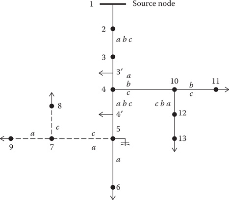
FIGURE 10.4
Typical distribution feeder.

In Figure 10.4, no distinction is made as to what type of element is connected between nodes. However, the phasing is shown, and this is a must. All series elements (lines, transformers, regulators) can be represented by the circuit in Figure 10.5. Note in Figure 10.4 that the lines between nodes 3 and 4 and between nodes 4 and 5 have “distributed” loads modeled at the middle of the lines. The model for the distributed loads was developed in Chapter 3. Connecting the loads at the center was only one of the three ways to model the load. A second method is to place one-half of the load at each end of the line. The third method is to place two-thirds of the load 25% of the way down the line from the source end. The remaining one-third of the load is connected at the receiving-end node. This “exact” model gives the correct voltage drop down the line in addition to the correct power-line power loss.

images

FIGURE 10.5
Standard feeder series component model.

In previous chapters, the forward and backward sweep models have been developed for the series elements. With reference to Figure 10.5, the forward and backward sweep equations are:

$\begin{array}{l} Forward sweep: {[V L N_{a b c}]}_{n} = [A] \cdot {[V L N_{a b c}]}_{m} - [B] \cdot {[I_{a b c}]}_{n} \\ Backward sweep: {[I_{a b c}]}_{n} = [c] \cdot {[V L N_{a b c}]}_{m} + [d] \cdot {[I_{a b c}]}_{n} \end{array}$ (10.7)

In most cases, the $[c]$ matrix will be zero. Long underground lines will be the exception. It was also shown that for the grounded wye–delta transformer bank, the backward sweep equation is:

${[I_{a b c}]}_{n} = [x_{t}] \cdot {[V L N_{a b c}]}_{n} + [d] \cdot {[I_{a b c}]}_{m}$ (10.8)

The reason for this is that the currents flowing in the secondary delta windings are a function of the primary line-to-ground voltages.

Referring to Figure 10.4, nodes 4, 10, 5, and 7 are referred to as “junction nodes.” In both the forward and backward sweeps, the junction nodes must be recognized. In the forward sweep, the voltages at all nodes down the lines from the junction nodes must be computed. In the backward sweeps, the currents at the junction nodes must be summed before proceeding toward the source. In developing a program to apply the modified ladder method, it is necessary for the ordering of the lines and nodes to be such that all node voltages in the forward sweep are computed and all currents in the backward sweep are computed.

10.1.3 The Unbalanced Three-Phase Distribution Feeder

The previous section outlined the general procedure for performing the modified ladder iterative technique. This section will address how that procedure can be used for an unbalanced three-phase feeder.

Figure 10.6 is the one-line diagram of an unbalanced three-phase feeder as shown in Figure 10.5.

images

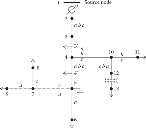
FIGURE 10.6
Unbalanced three-phase distribution feeder.

The topology of the feeder in Figure 10.6 is the same as the feeder in Figure 10.5. Figure 10.6 shows more details of the feeder with step regulators at the source and a transformer bank at node 12. The feeder in Figure 10.6 can be broken into the “series” components and the “shunt” components. The series components have been shown in Section 10.1.2.

10.1.3.1 Shunt Components

The shunt components of a distribution feeder are:

Spot static loads
Spot induction machines
Capacitor banks

Spot static loads are located at a node and can be three-phase, two-phase, or single-phase, and connected in either a wye or a delta connection. The loads can be modeled as constant complex power, constant current, constant impedance, or a combination of the three.

A spot induction machine is modeled using the shunt admittance matrix as defined in Chapter 9. The machine can be modeled as a motor with a positive slip or as an induction generator with a negative slip. The input power (positive for a motor, negative for a generator) can be specified, and the required slip is computed using the iterative process described in Chapter 9.

Capacitor banks are located at a node and can be three-phase, two-phase, or single-phase, and can be connected in a wye or delta. Capacitor banks are modeled as constant admittances.

In Figure 10.6, the solid line segments represent overhead lines, while the dashed lines represent underground lines. Note that the phasing is shown for all of the line segments. In Chapter 4, the application of Carson’s equations for computing the line impedances for overhead and underground lines was presented. In that chapter, it is pointed out that two-phase and single-phase lines are represented by a 3 × 3 matrix with zeros set in the rows and columns of the missing phases.

In Chapter 5, the method for the computation of the shunt capacitive susceptance for overhead and underground lines was presented. Most of the times, the shunt capacitance of the line segment can be ignored; however, for long underground line segments, the shunt capacitance should be included.

The “node” currents may be three-phase, two-phase, or single-phase and consist of the sum of the spot load currents and one-half of the distributed load currents (if any) at the node plus the capacitor current (if any) at the node. It is possible that at a given node, the distributed load can be one-half of the distributed load in the “from” segment plus one-half of the distributed load connected to the “to” segment. In some cases, a “dummy” node is created in the center of the line, and the total distributed load is connected to this node.

10.1.4 Applying the Ladder Iterative Technique

Section 10.1.2 outlined the steps required for the application of the ladder iterative technique. Forward and backward sweep matrices have been developed in Chapters 6, 7, and 8 for the series devices. By applying these matrices, the computation of the voltage drops along a segment will always be the same regardless of whether the segment represents a line, voltage regulator, or transformer.

In the preparation of data for a power-flow study, it is extremely important that the impedances and admittances of the line segments are computed using the exact spacings and phasing. Because of the unbalanced loading and resulting unbalanced line currents, the voltage drops due to the mutual coupling of the lines become very important. It is not unusual to observe a voltage rise on a lightly loaded phase of a line segment that has an extreme current unbalance.

The real power loss in a device can be computed in two ways. The first method is to compute the power loss in each phase by taking the phase current squared times the total resistance of the phase. Care must be taken to not use the resistance value from the phase impedance matrix. The actual phase resistance that was used in Carson’s equations must be used. Developing a computer program calculating power loss this way requires that the conductor resistance is stored in the active database for each line segment. Unfortunately, this method does not give the total power loss in a line segment, since the power losses in the neutral conductor and ground are not included. In order to determine the losses in the neutral and ground, the method outlined in Chapter 4 must be used to compute the neutral and ground currents and then the power losses.

A second, and preferred, method is to compute the power loss as the difference of real power into a line segment minus the real power output of the line segment. Because the effects of the neutral conductor and ground are included in the phase impedance matrix, the total power loss in this method will give the same results as mentioned earlier, where the neutral and ground power losses are computed separately. This method can lead to some interesting numbers for very unbalanced line flows in that it is possible to compute what appears to be a negative phase power loss. This is a direct result of the accurate modeling of the mutual coupling between phases. Remember that the effects of the neutral conductor and the ground resistance are included in Carson’s equations. In reality, there cannot be a negative phase power loss. Using this method, the algebraic sum of the line power losses will equal the total three-phase power loss that was computed using the current squared times resistance for the phase and neutral conductors along with the ground current.

10.1.5 Let’s Put It All Together

At this point, the models for all components of a distribution feeder have been developed. The ladder iterative technique has also been developed. It is time to put them all together and demonstrate the power-flow analysis of a very simple system. Example 10.2 will demonstrate how the models of the components work together in applying the ladder technique to achieve a final solution of the operating characteristics of an unbalanced feeder.

Example 10.2

A very simple distribution feeder is shown in Figure 10.7. This system is the IEEE 4 Node Test Feeder that can be found on the IEEE website [3].

images

FIGURE 10.7
Example 10.2 feeder.

For the system in Figure 10.7, the infinite bus voltages are balanced three-phase of 12.47 kV line-to-line. The “source” line segment from node 1 to node 2 is a three-wire delta 2000 ft long line and is constructed on the pole configuration in Figure 4.7 without the neutral. The “load” line segment from node 3 to node 4 is 2500 ft long and is also constructed on the pole configuration in Figure 4.7 but is a four-wire wye; so the neutral is included. Both line segments use 336,400 26/7 ACSR phase conductors, and the neutral conductor on the four-wire wye line is 4/0 6/1 ACSR. Because the lines are short, the shunt admittance will be neglected. The 25°C resistance is used for the phase and neutral conductors:

336,400 26/7 ACSR: resistance at 25°C = 0.278 Ω/mile

4/0 6/1 ACSR: resistance at 25°C = 0.445 Ω/mile

The phase impedance matrices for the two line segments are:

$[Z {eq}_{S}] = [\begin{matrix} 0.1414 + j 0.5353 & 0.0361 + j 0.3225 & 0.0361 + j 0.2752 \\ 0.0361 + j 0.3225 & 0.1414 + j 0.5353 & 0.0361 + j 0.2955 \\ 0.0361 + j 0.2752 & 0.0361 + j 0.2955 & 0.1414 + j 0.5353 \end{matrix}] Ω$

$[Z {eq}_{L}] = [\begin{matrix} 0.1907 + j 0.5035 & 0.0607 + j 0.2302 & 0.0598 + j 0.1751 \\ 0.0607 + j 0.2302 & 0.1939 + j 0.4885 & 0.0614 + j 0.1931 \\ 0.0598 + j 0.1751 & 0.0614 + j 0.1931 & 0.1921 + j 0.4970 \end{matrix}] Ω$

The transformer bank is connected delta-grounded wye and the three-phase ratings are:

$k V A = 6000, k V L L_{S} = 12.47, k V L L_{L} = 4.16, Z_{pu} = 0.01 + j 0.06$

The feeder serves an unbalanced three-phase wye-connected constant PQ load of:

S_a = 750 kVA at 0.85 lagging power factor

S_b = 900 kVA at 0.90 lagging power factor

S_c = 1100 kVA at 0.95 lagging power factor

Before starting the iterative solution, the forward and backward sweep matrices must be computed for each series element. The ladder method is going to be employed; therefore, only the $[A], [B], and [d]$ matrices need to be computed.

Source line segment with shunt admittance neglected:

$[U] = [\begin{matrix} 1 & 0 & 0 \\ 0 & 1 & 0 \\ 0 & 0 & 1 \end{matrix}]$

$[A_{1}] = [U] = [\begin{matrix} 1 & 0 & 0 \\ 0 & 1 & 0 \\ 0 & 0 & 1 \end{matrix}]$

$[B_{1}] = [Z_{{eq}_{S}}] = [\begin{matrix} 0.1414 + j 0.5353 & 0.0361 + j 0.3225 & 0.0361 + j 0.2752 \\ 0.0361 + j 0.3225 & 0.1414 + j 0.5353 & 0.0361 + j 0.2955 \\ 0.0361 + j 0.2752 & 0.0361 + j 0.2955 & 0.1414 + j 0.5353 \end{matrix}]$

$[d_{1}] = [U] = [\begin{matrix} 1 & 0 & 0 \\ 0 & 1 & 0 \\ 0 & 0 & 1 \end{matrix}]$

Load line segment:

$[A_{2}] = [U] = [\begin{matrix} 1 & 0 & 0 \\ 0 & 1 & 0 \\ 0 & 0 & 1 \end{matrix}]$

$[B_{2}] = [Z {eq}_{L}] [\begin{matrix} 0.1907 + j 0.5035 & 0.0607 + j 0.2302 & 0.0598 + j 0.1751 \\ 0.0607 + j 0.2302 & 0.1939 + j 0.4885 & 0.0614 + j 0.1931 \\ 0.0598 + j 0.1751 & 0.0614 + j 0.1931 & 0.1921 + j 0.4970 \end{matrix}]$

$[d_{2}] = [U] = [\begin{matrix} 1 & 0 & 0 \\ 0 & 1 & 0 \\ 0 & 0 & 1 \end{matrix}]$

Transformer:

The transformer impedance must be converted to actual value in ohms referenced to the low-voltage windings.

$Z_{base} = \frac{k V L L_{L}^{2} \cdot 1000}{k V A} = 2.88 Ω$

$Z t_{_{low}} = (0.01 + j 0.06) \cdot 2.88 = 0.0288 + j 0.1728 Ω$

The transformer phase impedance matrix is:

$[Z t_{_{a b c}}] = [\begin{matrix} 0.0288 + j 0.1728 & 0 & 0 \\ 0 & 0.0288 + j 0.1728 & 0 \\ 0 & 0 & 0.0288 + j 0.1728 \end{matrix}] Ω$

The “turns” ratio:

$n_{t} = \frac{k V L L_{S}}{k V L N_{L}} = 5.1958$

The ladder sweep matrices are:

$[A_{t}] = \frac{1}{n_{t}} \cdot [\begin{matrix} 1 & 0 & - 1 \\ - 1 & 1 & 0 \\ 0 & - 1 & 1 \end{matrix}] = [\begin{matrix} 0.1925 & 0 & - 0.1925 \\ - 0.1925 & 0.1925 & 0 \\ 0 & - 0.1925 & 0.1925 \end{matrix}]$

$[B_{t}] = [Z t_{_{a b c}}] = [\begin{matrix} 0.0288 + j 0.1728 & 0 & 0 \\ 0 & 0.0288 + j 0.1728 & 0 \\ 0 & 0 & 0.0288 + j 0.1728 \end{matrix}]$

$[d_{t}] = \frac{1}{n_{t}} \cdot [\begin{matrix} 1 & - 1 & 0 \\ 0 & 1 & - 1 \\ - 1 & 0 & 1 \end{matrix}] = [\begin{matrix} 0.1925 & - 0.1925 & 0 \\ 0 & 0.1925 & - 0.1925 \\ - 0.1925 & 0 & 0.1925 \end{matrix}]$

Define the node 4 loads:

$[S_{4}] = [\begin{matrix} 750 \underset{___________}{/ acos (0.85)} \\ 900 \underset{___________}{/ acos (0.90)} \\ 1100 \underset{___________}{/ acos (0.95)} \end{matrix}] = [\begin{matrix} 750 \underset{______}{/ 31.79} \\ 900 \underset{______}{/ 25.84} \\ 1100 \underset{______}{/ 18.19} \end{matrix}] = [\begin{matrix} 637.5 + j 395.1 \\ 810.0 + j 392.3 \\ 1045.0 + j 343.5 \end{matrix}] kVA$

Define infinite bus line-to-line and line-to-neutral voltages:

$[E L L_{s}] = [\begin{matrix} 12, 470 \underset{___}{/ 30} \\ 12, 470 \underset{____}{/ - 90} \\ 12, 470 \underset{____}{/ 150} \end{matrix}] V$

$[E L N_{s}] = [\begin{matrix} 7199.6 \underset{__}{/ 0} \\ 7199.6 \underset{_____}{/ - 120} \\ 7199.6 \underset{____}{/ 120} \end{matrix}] V$

The initial conditions are:

$Start = [\begin{matrix} 0 \\ 0 \\ 0 \end{matrix}] Tol = 0.00001 V M = 7199.6$

A Mathcad program is shown in Figure 10.8.

The Mathcad program is used to analyze the system, and after seven iterations, the load voltages on a 120-V base are:

$[V 4_{_{120}}] = [\begin{matrix} 113.4 \\ 111.5 \\ 112.0 \end{matrix}] V$

The voltages at node 4 are below the desired 120 V. These low voltages can be corrected with the installation of three step-voltage regulators connected in wye on the secondary bus (node 3) of the transformer. The new configuration of the feeder is shown in Figure 10.9.

images

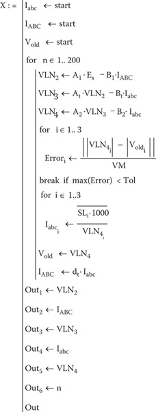
FIGURE 10.8
Mathcad program.

images

FIGURE 10.9
Voltage regulator added to the system.

For the regulator, the potential transformer ratio will be 2400–120 V (N_pt = 20), and the CT ratio is selected to carry the rated current of the transformer bank. The rated current is:

$I_{rated} = \frac{6000}{\sqrt{3} \cdot 2.4} = 832.7$

The CT ratio is selected to be 1000:5 = CT = 200.

The potential transformer ratio is: $N_{p t} = \frac{V L N_{rated}}{120} = \frac{2400}{120} = 20$

The equivalent phase impedance between nodes 3 and 4 is computed using the converged voltages at the two nodes. This is done so that the R and X settings of the compensator can be determined.

$Z_{{eq}_{i}} = \frac{V 3_{_{i}} - V 4_{_{i}}}{I 3_{_{i}}} = [\begin{matrix} 0.1563 + j 0.2184 \\ 0.1837 + j 0.2860 \\ 0.0919 + j 0.3695 \end{matrix}] Ω$

The three regulators are to have the same R and X compensator settings. The average value of the computed impedances will be used.

$Z_{avg} = \frac{1}{3} \cdot \sum_{k = 1}^{3} Z {eq}_{_{k}} = 0.1440 + j 0.2913 Ω$

The value of the compensator impedance in volts is given by Equation 7.78:

$R^{'} + j X^{'} = (0.1440 + j 0.2913) \cdot \frac{1000}{20} = 7.2 + j 14.6 V$

The value of the compensator settings in ohms is:

$Z_{comp} = R_{Ω} + j X_{Ω} = \frac{7.2 + j 14.6}{5} = 1.44 + j 2.92 Ω$

With the regulator in the neutral position, the voltages being input to the compensator circuit for the given conditions are:

$V {reg}_{i} = \frac{V 3_{_{i}}}{P T} = [\begin{matrix} 117.5 \underset{______}{/ - 31.2} \\ 117.4 \underset{_______}{/ - 151.5} \\ 117.2 \underset{_____}{/ 88.0} \end{matrix}] V$

The compensator currents are:

$I {comp}_{i} = \frac{I a b c_{_{i}}}{C T} = [\begin{matrix} 1.6535 \underset{______}{/ - 63.8} \\ 2.0174 \underset{_______}{/ - 179.1} \\ 2.4560 \underset{_____}{/ 64.9} \end{matrix}] A$

With the input voltages and compensator currents, the voltages across the voltage relays in the compensator circuit are computed to be:

$[V_{relay}] = [V reg] - [Z comp] \cdot [I comp] = [\begin{matrix} 113.0 \underset{______}{/ - 32.6} \\ 112.2 \underset{_______}{/ - 153.5} \\ 111.4 \underset{_____}{/ 85.3} \end{matrix}] V$

Notice how close these compare to the actual voltages on a 120-V base at node 4.

Assume that the voltage level has been set at 121 V with a bandwidth of 2 V. This means that the relay voltages must lie between 120 and 122 V. In order to model this system, the Mathcad routine in Figure 10.8 is slightly modified in the forward and backward sweeps. The initial matrices for the regulator are computed with the regulator taps set at zero.

Forward sweep

$\begin{array}{l} [V L N_{2}] = [A_{1}] \cdot [E_{s}] - [B_{1}] \cdot [I_{A B C}] \\ [V L N_{3 r}] = [A_{t}] \cdot [V L N_{2}] - [B_{t}] \cdot [I_{i n}] \\ [V L N_{3}] = [A_{reg}] [V L N_{3}] - [B_{reg}] \cdot [I_{a b c}] \\ [V L N_{4}] = [A_{2}] \cdot [V L N_{3}] - [B_{2}] \cdot [I_{a b c}] \end{array}$

Backward sweep

$\begin{array}{l} [V_{old}] = [V L N_{4}] \\ [I_{in}] = [d_{reg}] \cdot [I_{a b c}] \\ [I_{A B C}] = [d_{t}] \cdot [I_{in}] \end{array}$

After the analysis routine has converged, a new routine will compute whether or not tap changes need to be made. The Mathcad routine for computing the new taps is shown in Figure 10.10. Recall that in Chapter 7 it was shown that each tap changes the relay voltages by 0.75 V.

The computational sequence for the determination of the final tap settings and convergence of the system is shown in the flowchart in Figure 10.11.

images

FIGURE 10.10
Tap-changing routine.

The tap-changing routine changes individual regulators, so that the relay voltages lie within the voltage bandwidth. For this simple system, the initial change in taps becomes the final tap settings of:

$[Tap] = [\begin{matrix} 9 \\ 10 \\ 11 \end{matrix}]$

The final relay voltages are:

$[V_{relay}] = [\begin{matrix} 120.3 \\ 120.5 \\ 120.6 \end{matrix}]$

The final voltages on a 120-V base at the load center (node 4) are:

$[V L N_{4_{120}}] = [\begin{matrix} 120.6 \\ 119.8 \\ 121.2 \end{matrix}]$

images

Figure 10.11
Computational sequence.

The compensator relay voltages and the actual load center voltages are very close to each other.

10.1.6 Load Allocation

Many times, the input complex power (kW and kvar) to a feeder is known because of the metering at the substation. This information can be either for the total three-phase or for each individual phase. In some cases, the metered data may be the current and power factor in each phase.

It is desirable to force the computed input complex power to the feeder to match the metered input. This can be accomplished (following a converged iterative solution) by computing the ratio of the metered input to the computed input. The phase loads can now be modified by multiplying the loads by this ratio. Because the losses of the feeder will change when the loads are changed, it is necessary to go through the ladder iterative process to determine a new computed input to the feeder. This new computed input will be closer to the metered input but most likely not within a specified tolerance. Following another ladder iteration, a ratio can be determined, and the loads modified followed. This process is repeated until the computed input is within a specified tolerance of the metered input.

Load allocation does not have to be limited to match metered readings just at the substation. The same process can be performed at any point on the feeder where metered data are available. The only difference is that now the “downstream” nodes from the metered point will be modified.

10.1.7 Loop Flow

The ladder interactive technique has proven to be a fast and efficient method for performing power-flow studies on radial distribution feeders. The shortcoming for this method is that there are cases where a feeder is not completely radial, and therefore a different method must be applied. Many times, the feeder may have just a few loops, in which case the ladder method can be modified to take into account the small looped feeder. A method called “loop flow” will be developed that will allow for loops in a predominately radial feeder [5].

10.1.7.1 Single-Phase Feeder

Figure 10.12 shows two small single-phase systems operating independently but with a switch between the two that once closed the two small systems become one looped system. When the switch is closed, the difference voltage ( $d V_{34}$ ) will be zero. Something has to be done to the system in order to force the difference voltage to be zero.

A way to simulate the closed switch is illustrated in Figure 10.13.

images

FIGURE 10.12
Single-phase system with a loop.

images

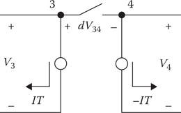
FIGURE 10.13
Simulation of closed switch.

To simulate the closed switch in Figure 10.13, it is necessary to determine the correct value of $I T$ to be injected into node 3 and the negative of $I T$ to be injected into node 4 that will force the voltage $d V_{34}$ to be zero. The circuit in Figure 10.12 is modified to include the injected currents at nodes 3 and 4.

images

FIGURE 10.14
Modified circuit.

In Figure 10.14, the voltages at nodes 3 and 4 are given by:

$\begin{array}{l} V_{3} = E_{1} - Z_{12} \cdot (I L_{2} + I T) - Z_{23} \cdot I T \\ V_{3} = E_{1} - Z_{12} \cdot I L_{2} - (Z_{12} + Z_{23}) \cdot I T \\ Define: \\ V_{3 V} = E_{1} - Z_{12} \cdot I L_{_{2}} \\ V_{3 I} = - (Z_{12} + Z_{23}) \cdot I T \\ Therefore: \\ V_{3} = V_{3 V} + V_{3 I} \end{array}$ (10.9)

In a similar manner, the voltage at node 4 is computed as:

$\begin{array}{l} V_{4} = E_{2} - Z_{56} \cdot (I L_{_{5}} - I T) - Z_{45} \cdot (- I T) \\ V_{4} = E_{2} - Z_{56} \cdot I_{L_{5}} + (Z_{56} + Z_{45}) \cdot I T \\ Define: \\ V_{4 V} = E_{2} - Z_{56} \cdot I_{L 5} \\ V_{4 I} = + (Z_{56} + Z_{45}) \cdot I T \\ Therefore: \\ V_{4} = V_{4 V} + V_{4 I} \end{array}$ (10.10)

The voltage drop between nodes 3 and 4 consists of a component due to the source voltages and a component due to the injected currents. Using the final form of the node voltages, the difference voltage between nodes 3 and 4 is given by:

$\begin{array}{l} V_{3} = V_{3 V} + V_{3 I} \\ V_{4} = V_{4 V} + V_{4 I} \\ d V_{34} = V_{3} - V_{4} = V_{3 V} - V_{4 V} + (V_{3 I} - V_{4 I}) \\ d V_{34} = d V_{34 V} + d V_{34 I} \end{array}$ (10.11)

Applying Equations 10.9 and 10.10, the difference voltage resulting from the application of the injection currents is given by:

$\begin{array}{l} d V_{34 I} = V_{3 I} - V_{4 I} = - (Z_{12} + Z_{23} + Z_{56} + Z_{45}) \cdot I T \\ d V_{34 I} = - Thev Z \cdot I T \\ where Thev Z = Z_{12} + Z_{23} + Z_{56} + Z_{45} \end{array}$ (10.12)

For this simple system, $Thev Z$ is the sum of the line impedances around the closed loop. This impedance is referred to as the Thevenin equivalent impedance. For a general system, the impedance is computed by the principle of superposition, where the voltage sources are set to zero, the loads neglected, and only the injected currents are applied to the system. For this simple system, such a circuit is shown in Figure 10.15.

Equation 10.12 applies KVL around the looped system in Figure 10.15. With the voltage drop $d V_{34 I}$ computed, the Thevenin equivalent impedance is computed as:

$Thev Z = \frac{- d V_{34 I}}{I T}$ (10.13)

With $Thev Z$ computed, the final goal is to determine the value of $I T$ that will force the difference voltage to be zero as shown in Equation 10.14.

$\begin{array}{l} 0 = d V_{34 V} + d V_{34 I} \\ d V_{34 I} = - d V_{34 V} \\ where: d V_{34 I} = - Thev Z \cdot I T \\ therefore: - d V_{34 V} = - Thev Z \cdot I T \\ I T = \frac{d V_{34 V}}{Thev Z} \end{array}$ (10.14)

images

FIGURE 10.15
Thevenin equivalent impedance circuit.

Because the loads on a distribution system are nonlinear, an iterative routine is used to compute the needed injection currents. Figure 10.16 shows a simple flowchart of an iterative routine used to compute the injected currents.

images

FIGURE 10.16
Flowchart for solution with injected currents.

It is noted in Figure 10.16 that the initial injection currents are set to zero. During the first iteration, the difference voltage will be a function of only the source voltages and the load currents. With this difference voltage computed, the first value of the injection currents is computed according to Equation 10.14 and then added to the initial value of $I T = 0$ . With the new value of injection currents, the circuit in Figure 10.14 is evaluated to compute the new difference voltage, which now includes the effect of the injection currents. The new difference voltage is checked to see whether it is within a specified tolerance of the desired zero. If it is not, an additional injection current is computed and added to the most recent value of the injection currents.

This simple single-phase circuit was used to demonstrate a method of simulating a looped system. To demonstrate how this approach is used in a larger system, the IEEE 13 Bus Test Feeder will be studied [4].

Example 10.3

Determine the values of the injected currents for the system in Figure 10.14 to simulate loop flow between the two sources.For the system, the following data are given:

$E_{1} = 7200 V, E_{2} = 1.05 \cdot E_{1} = 7560 V$

Impedance of the lines:

$z_{1} = 0.5152 + j 1.1359 Ω /mile$

Length of lines:

$L_{12} = 5, L_{23} = 2, L_{45} = 3, L_{56} = 4 miles$

Line impedances:

$\begin{matrix} Z_{12} = 0.2576 + j 0.5679 \\ Z_{23} = 1.0304 + j 2.2718 \\ Z_{45} = 1.5456 + j 3.4077 \\ Z_{56} = 2.0608 + j 4.5436 \end{matrix} Ω$

Loads:

$\begin{matrix} S_{L_{2}} = 1500 + j 1250 \\ S_{L_{_{5}}} = 1000 + j 750 \end{matrix} kW + j k v a r$

Step 1: Set the voltage sources to zero, and apply the positive and negative injection currents.

The base values are:

$\begin{array}{l} k V A_{base} = 1000, k V_{L N_{base}} = 7.2 \\ I_{base} = \frac{k V A_{base}}{k V_{L N_{base}}} = 138.9 \end{array}$

The injected current magnitude is set to the base current:

$\begin{array}{l} I T_{1} = I_{base} = 138.9 \\ I T_{2} = - I T_{1} = - 138.9 \end{array}$

The analysis of the system with the two injected currents gives:

$\begin{array}{l} V_{3 I} = 433.1 \underset{_______}{/ - 114.4} \\ V_{4 I} = 1212.6 \underset{_____}{/ 65.6} \\ d V_{34 I} = V_{3 I} - V_{4 I} = 1645.7 / - 114.4 \end{array}$

The Thevenin equivalent impedance is:

$Z_{t h} = \frac{- d V_{34 I}}{I T} = \frac{1645.7 \underset{_______}{/ - 114.4}}{138.9 \underset{__}{/ 0}} = 4.8944 + j 10.7911$

Step 2: Set the injected currents to zero and compute $d V_{34}$

With the injected currents equal to zero, a Mathcad routine computes the voltages as:

$\begin{array}{l} V_{3 V} = 7043.97 \underset{_____}{/ - 0.6} \\ V_{4 V} = 6734.96 \underset{____}{/ - 3.4} \\ d V_{34 V} = V_{3 V} - V_{4 V} = 454.86 \underset{_____}{/ 45.2} \end{array}$

With the equivalent Thevenin impedance computed, the first value of the required injected current is:

$\begin{array}{l} I T_{add} = \frac{V_{34 V}}{Z_{t h}} = 38.39 \underset{______}{/ - 20.4} \\ I T = I T + I T_{add} = 0 + 38.39 \underset{______}{/ - 20.4} = 38.39 \underset{______}{/ - 20.4} \end{array}$

The difference voltage is now computed with the voltage sources and injected currents. After this first iteration, the difference voltage is computed to be:

$\begin{array}{l} V_{3} = 6958.3 \underset{_____}{/ - 1.3} \\ V_{4} = 7007.5 \underset{_____}{/ - 1.4} \\ d V_{34} = 50.6 \underset{_____}{/ 164.9} \end{array}$

The added injection current and new total injected current is:

$\begin{array}{l} I T_{add} = \frac{50.6 \underset{______}{/ 164.9}}{11.85 \underset{______}{/ 65.60}} = 4.28 \underset{______}{/ 99.27} \\ I T = I T + I T_{add} = 38.39 / - 20.4_+ 4.28 \underset{______}{/ 99.27} = 36.46 \underset{_______}{/ - 14.52} \end{array}$

The difference voltage is again computed using the new value of injected current. This process continues until after the fifth iteration when the difference voltage is:

$\begin{array}{l} V_{3} = 6970.42 . \underset{______}{/ - 1.33} \\ V_{4} = 6970.42 . \underset{______}{/ - 1.33} \\ d V_{34} = V_{3} - V_{4} = 0 \end{array}$

The line currents flowing with injected currents are:

$\begin{array}{l} I_{23} = 36.8842 \underset{_______}{/ - 14.65} \\ I_{45} = 36.8842 \underset{_______}{/ - 14.65} \end{array}$

Because these two currents are identical, the two systems are now operating as one system, with system 1 providing current to system 2 just as though the switch between nodes 3 and 4 was closed.

10.1.7.2 IEEE 13 Bus Test Feeder

The IEEE 13 Bus Test Feeder was developed to allow distribution analysis programs to be tested with the results compared to the published results. This feeder will be used to demonstrate the simulation of a looped system using the method presented in the previous section. A one-line diagram of the IEEE 13 Bus Test Feeder is shown in Figure 10.17 [3].

images

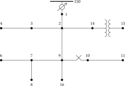
FIGURE 10.17
IEEE 13 Bus Test Feeder.

Example 10.4

The system in Figure 10.17 was created in Windmil. With the original data, partial results are shown in Table 10.1. The currents are in amps, and the voltages are line-to-neutral on a 120-V base.

TABLE 10.1
Original Feeder Results

images

As seen in Table 10.1, the voltages are very unbalanced at Bus 11. This unbalance was purposely created so that distribution analysis programs could be tested for convergence in a very unbalanced feeder. No effort will be made in this text to balance the voltages. Even though the voltages are unbalanced, they are still within the ANSI standard [5] of all voltages being between 114 and 126 V.

Rather than balance the voltages, two new loads are going to be added to the existing feeder, which will lead to the need for the looped feeder. The following loads are added to the system:

Bus 6: Phase c: 200+ j100kW+ jkvar

Bus 11: Three-phase load: 750+ j525 kW + jkvar

With the new loads and the voltage regulator operating, the partial results are shown in Table 10.2.

The voltage at Bus 6 has gone below the ANSI minimum of 114 V. The voltage at Bus 11 Phase c is also below the ANSI standard. The actual problem with Bus 11 is that the current capacity of 260 A on the underground concentric neutral cable between Bus 10 and Bus 11 is exceeded. In order to solve these problems and to demonstrate the looped feeder simulation, two new lines will be added to the system. The one-line diagram of the modified IEEE 13 feeder is shown in Figure 10.18.

TABLE 10.2
New Loads Added

images

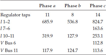
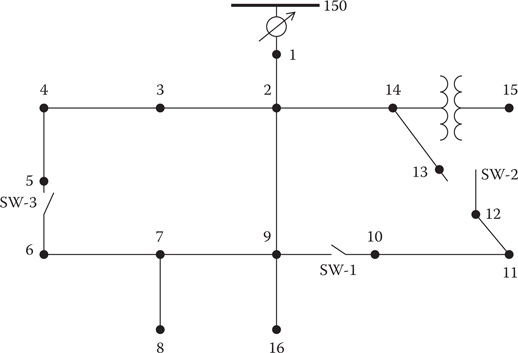
FIGURE 10.18
Modified IEEE 13 Bus Test Feeder.

The new line from Bus 4 to Bus 5 consists of 1/0 ACSR 6/1 constructed on a single pole as shown in Figure 10.19. The length of the line is 600ft.

The three-phase line from Bus 14 to Bus 13 consists of 4/0 ACSR 6/1 phase and neutral conductors with a pole configuration as shown in Figure 10.20. The length of the line is 800 ft.

In order to simulate the loop flow, currents must be injected into Buses 5, 6, 13, and 11 as shown in Figure 10.21.

The line from Bus 2 to bus 9 has a distributed load, which is modeled as two-thirds of the distributed load at Bus 2a, which is one-third the length of the line, and the remaining distributed load is connected at the end of the line at the new Bus 9a. In Figure 10.21, SW-1 is a three-phase switch that can only be modeled as open or closed. SW-2 is a three-phase switch that can be modeled as open, closed, or looped. SW-3 is a single-phase switch on phase c and can only be modeled as open or looped.

images

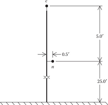
FIGURE 10.19
Single-phase line.

images

FIGURE 10.20
Three-phase line.

images

FIGURE 10.21
Injected currents.

The first step in simulating loop flow is to compute the Thevenin equivalent impedance at each looped switch for each phase. The currents injected into Bus 13 (IT1) will be in phases a, b, and c. The injected currents at Bus 11 (IT3) will be the negative of IT1. Switch SW-3 is a single-phase switch on Phase c. Therefore, the injected current at Bus 5 (IT2) will only be a Phase c current. The injected current at Bus 6 (IT4) will be the negative of IT2. There will be a Thevenin equivalent impedance computed at each switch for each phase injected at each of the injection nodes. This will lead to a 4 × 4 Thevenin equivalent matrix (ThevZ). For this process, the value of the injected current is assumed to be the base current of the system 694.4 A.

For the computation of $Thev Z$ , the source voltages and all loads are set to zero. Refer to Figure 10.21 with SW-1 closed. The line-to-neutral voltages at Buses 13, 11, 5, and 6 are computed with only the Phase a currents being injected at Buses 13 and 12. A Mathcad program is used to compute the voltages. With only the Phase a currents, the vectors for the injected currents at the switch buses are:

$[I T 1] = [\begin{matrix} 694.4 \\ 0 \\ 0 \end{matrix}] [I T 3] = [\begin{matrix} - 694.4 \\ 0 \\ 0 \end{matrix}]$ (10.15)

The bus voltages with just the Phase a-injected current at Bus 13 are computed to be:

$\begin{array}{l} [V_{13}] = [\begin{matrix} 239.5 \underset{_______}{/ - 122.5} \\ 77.3 \underset{_______}{/ - 110.5} \\ 89.8 \underset{______}{/ - 107.3} \end{matrix}] [V_{12}] = [\begin{matrix} 330.0 \underset{_____}{/ 64.2} \\ 147.8 \underset{_____}{/ 65.2} \\ 125.9 \underset{_____}{/ 61.4} \end{matrix}] \\ [V_{5 c}] = 0 [V_{6 c}] = 118.9 \underset{_______}{/ - 110.5} \end{array}$ (10.16)

The difference voltages are:

$\begin{array}{l} [d V_{1312}] = [\begin{matrix} 568.6 \underset{______}{/ - 118.6} \\ 224.9 \underset{______}{/ - 113.3} \\ 214.7 \underset{______}{/ - 113.9} \end{matrix}] \\ d V_{56 c} = 118.93 \underset{_______}{/ - 110.5} \end{array}$ (10.17)

Equation 10.17 is used to compute the first column elements of the $T h e v Z$ matrix.

$\begin{matrix} [\begin{matrix} Thev Z_{1, 1} \\ Thev Z_{2, 1} \\ Thev Z_{3, 1} \end{matrix}] = - \frac{1}{I T} \cdot [\begin{matrix} d V_{1312 a} \\ d V_{1312 b} \\ d V_{1312 c} \end{matrix}] = [\begin{matrix} 0.3921 + j 0.7187 \\ 0.1282 + j 0.2974 \\ 0.1252 + j 0.2826 \end{matrix}] \\ Thev z_{4, 1} = \frac{- d V_{56 c}}{I T} = 0.0598 + j 0.1605 \end{matrix} Ω$ (10.18)

This process is repeated with the injected currents in Phase b at Buses 13 and 12, followed by the injected currents in Phase c at Buses 13 and 12. The last step is to have the Phase c currents injected at Buses 5 and 6. The final $Thev Z$ matrix in ohms is:

$[Thev Z] = [\begin{matrix} 0.3921 + j 0.7178 & 0.1282 + j 0.2974 & 0.1252 + j 0.2826 & 0.0598 + j 0.1605 \\ 0.1282 + j 0.2974 & 0.3866 + j 0.7302 & 0.1262 + j 0.2437 & 0.0581 + j 0.1458 \\ 0.1252 + j 0.2826 & 0.1262 + j 0.2437 & 0.3880 + j 0.7324 & 0.1293 + j 0.3920 \\ 0.0598 + j 0.1605 & 0.0581 + j 0.1458 & 0.1293 + j 0.3920 & 0.6328 + j 0.9023 \end{matrix}]$ (10.19)

With TheZ computed, the values of the needed injection currents must be determined with the loads and capacitors included. The method is to apply Equation 10.18 in matrix form for the IEEE 13 bus feeder and solve for the [IT] array. The equation is:

$[\begin{matrix} I T 1_{a} \\ I T 1_{b} \\ I T 1_{c} \\ I T 2_{c} \end{matrix}] = {[T h e v Z]}^{- 1} \cdot [\begin{matrix} d V_{1311 a} \\ d V_{1311 b} \\ d V_{1311 c} \\ d V_{56 c} \end{matrix}]$ (10.20)

In order to determine the injection currents, the power-flow program must be run where all of the loads and capacitor along with the injection currents are modeled. The tap settings for the regulator are set at the same taps as in Table 10.2. As was done with the single-phase system, initially all of the injection currents are set to zero, and the difference voltages in Equation 10.20 are computed. Equation 10.20 is used to compute the initial change in injection currents. The computed difference voltages for this first iteration are:

$[\begin{matrix} d V_{1312 a} \\ d V_{1312 b} \\ d V_{1312 c} \\ d V_{56 c} \end{matrix}] = [\begin{matrix} 181.2 \underset{_____}{/ 50.8} \\ 39.4 \underset{_____}{/ - 17.4} \\ 206.2 \underset{______}{/ 151.8} \\ 228.7 \underset{______}{/ 153.6} \end{matrix}] V$ (10.21)

With the difference voltages computed, Equation 10.20 is used to compute the injection currents that will force the difference voltages to zero. During the first iteration, the injection currents were set to zero. Applying Equation 10.14 will give the “added” injection currents needed. After the first iteration, the computed injection currents are:

$[\begin{matrix} I T_{1 a} \\ I T_{1 b} \\ I T_{1 c} \\ I T_{2 c} \end{matrix}] = [\begin{matrix} 304.6 \underset{______}{/ - 22.0} \\ 145.5 \underset{_______}{/ - 122.4} \\ 261.7 \underset{______}{/ 102.8} \\ 147.4 \underset{_____}{/ 99.0} \end{matrix}] A$ (10.22)

With the currents in Equation 10.22 injected into the buses, the power-flow program is run again. Because the current flows on the lines will now be different, the bus voltages will also change. Because many of the loads are modeled as constant PQ, those load currents are subject to change. The second iteration is necessary to recalculate the bus voltages and determine whether additional injection currents are needed. After the second iteration, the difference voltages across the looped switches are:

$[\begin{matrix} d V_{1311 a} \\ d V_{1311 b} \\ d V_{1311 c} \\ d V_{56 c} \end{matrix}] = [\begin{matrix} 8.2 \underset{_______}{/ - 165.1} \\ 4.4 \underset{_______}{/ - 108.2} \\ 17.1 \underset{______}{/ - 76.8} \\ 18.1 \underset{______}{/ - 76.3} \end{matrix}] V$ (10.23)

Because the difference voltages are not close to zero, additional injection currents are needed. The additional currents are:

$[I T_{_{add}}] = [\begin{matrix} 15.1 \underset{_____}{/ 97.9} \\ 1.2 \underset{_____}{/ - 8.5} \\ 18.6 \underset{_______}{/ - 129.3} \\ 11.0 \underset{_______}{/ - 132.5} \end{matrix}] A$ (10.24)

The total injection currents for the next iteration are:

$[\begin{matrix} I T_{1 a} \\ I T_{1 b} \\ I T_{1 c} \\ I T_{2} \end{matrix}] = [\begin{matrix} 304.6 \underset{_____}{/ - 22.0} \\ 145.5 \underset{_______}{/ - 122.4} \\ 261.7 \underset{______}{/ 102.8} \\ 147.4 \underset{_____}{/ 99.0} \end{matrix}] + [\begin{matrix} 15.1 \underset{_____}{/ 97.9} \\ 1.2 \underset{____}{/ - 8.5} \\ 18.6 \underset{_____}{/ - 129.3} \\ 11.0 \underset{_______}{/ - 132.5} \end{matrix}] = [\begin{matrix} 297.4 \underset{______}{/ - 19.4} \\ 145.0 \underset{_______}{/ - 122.0} \\ 250.7 \underset{______}{/ 106.2} \\ 140.8 \underset{______}{/ 102.5} \end{matrix}]$ (10.25)

Following this procedure, after the fourth iteration, the difference voltages are very small, and the process stops. The injected currents and difference voltages are:

$\begin{array}{l} [\begin{matrix} I T_{1 a} \\ I T_{1 b} \\ I T_{1 c} \\ I T_{2 c} \end{matrix}] = [\begin{matrix} 298.0 \underset{______}{/ - 19.5} \\ 145.0 \underset{_______}{/ - 121.9} \\ 251.7 \underset{______}{/ 106.0} \\ 141.4 \underset{______}{/ 102.4} \end{matrix}] A \\ [\begin{matrix} d V_{1311 a} \\ d V_{1311 b} \\ d V_{1311 c} \\ d V_{56 c} \end{matrix}] = [\begin{matrix} 0.0276 \underset{_______}{/ - 121.2} \\ 0.0343 \underset{________}{/ - 93.9.6} \\ 0.0931 \underset{______}{/ - 62.4} \\ 0.0963 \underset{______}{/ - 62.2} \end{matrix}] V \end{array}$ (10.26)

In Table 10.2, it was shown that when the new loads were added at Buses 6 and 11, the bus voltage at Bus 6 was below the ANSI standard. Moreover, the concentric neutral line was overloaded. By adding the looped switches, Table 10.3 shows the results.

TABLE 10.3
Looped Switches

images

A comparison of Tables 10.2 and 10.3 shows the following:

The voltage at Bus 6 is now above the minimum ANSI standard of 114 V.
The current flowing in the concentric neutral cable from Bus 10 to Bus 11 is much lower than the cable current rating.
The voltages at Bus 11 are not as unbalanced and are somewhat higher.
The current out of the substation is basically the same, since the net injection currents are zero; so the slight change in this current is because of the change in load currents for the constant PQ loads.
The regulator tap positions have not changed, since the current into the line drop compensator is basically the same as that before the looped switches were closed.

10.1.7.3 Summary of Loop Flow

A method of simulating a looped distribution system has been presented. The loop is simulated by the installation of a switch between two existing buses in the feeder. To simulate the loop flow, the voltage at buses on the two sides of the switch must be equal. This is accomplished by the injection of a positive current at one of the buses and a negative value on the other bus. A method of calculating the necessary injection currents to force the difference voltage across the loop switch to be zero has been presented. Initially, a simple single-phase system was used to develop the technique. Following that, the IEEE 13 Bus Test Feeder was used to demonstrate the closing of a three-phase loop switch and a single-phase loop switch.

10.1.8 Summary of Power-Flow Studies

This section has developed a method for performing power-flow studies on a distribution feeder. Models for the various components of the feeder have been developed in previous chapters. The purpose of this section has been to develop and demonstrate the modified ladder iterative technique using the forward and backward sweep matrices for the series elements. It should be obvious that a study of a large feeder with many laterals and sublaterals cannot be performed without the aid of a complex computer program. In addition to the ladder iterative technique, a method of modeling a feeder with closed loops was presented under the name “loop flow.”

The development of the models and examples in this text use actual values of voltage, current, impedance, and complex power. When per-unit values are used, it is imperative that all values be converted to per-unit using a common set of base values. In the usual application of per-unit, there will be a base line-to-line voltage and a base line-to-neutral voltage; in addition, there will be a base line current and a base delta current. For both the voltage and current, there is a square root of three relationships between the two base values. In all of the derivations of the models, and in particular those for the three-phase transformers, the square root of three has been used to relate the difference in magnitudes between line-to-line and line-to-neutral voltages and between the line and delta currents. Because of this, when using the per-unit system, there should be only one base voltage, and that should be the base line-to-neutral voltage. When this is done, for example, the per-unit positive and negative sequence voltages will be the square root of three times the per-unit positive and negative sequence line-to-neutral voltages. Similarly, the positive and negative sequence per-unit line currents will be the square of three times the positive and negative sequence per-unit delta currents. By using just one base voltage and one base current, the per-unit generalized matrices for all system models can be determined.

10.2 Short-Circuit Studies

The computation of short-circuit currents for unbalanced faults in a normally balanced three-phase system has traditionally been accomplished by the application of symmetrical components. However, this method is not well suited to a distribution feeder that is inherently unbalanced. The unequal mutual coupling between phases leads to mutual coupling between sequence networks. When this happens, there is no advantage of using symmetrical components. Another reason for not using symmetrical components is that the phases between which faults occur are limited. For example, using symmetrical components line-to-ground faults are limited to phase a to the ground. What happens if a single-phase lateral is connected to Phase b or c and the short-circuit current is needed? This section will develop a method for short-circuit analysis of an unbalanced three-phase distribution feeder using the phase frame [4].

10.2.1 General Short-Circuit Theory

Figure 10.22 shows the unbalanced feeder as modeled for short-circuit calculations.

Short circuits can occur at any one of the five points shown in Figure 10.22. Point 1 is the high-voltage bus of the distribution substation transformer. The values of the short-circuit currents at point 1 are normally determined from a transmission system short-circuit study. The results of these studies are supplied in terms of the three-phase and single-phase short-circuit Mega-Volt-Amperes (MVAs). Using the short-circuit MVAs, the positive and zero sequence impedances of the equivalent system can be determined. These values are needed for the short-circuit studies at the other four points in Figure 10.22.

images

FIGURE 10.22
Unbalanced feeder short-circuit analysis model.

Given the three-phase short-circuit MVA magnitude and angle, the positive sequence equivalent system impedance in ohms is determined by:

$Z_{+} = \frac{k V_{L L}^{2}}{{(M V A_{3 -phase})}^{*}} Ω$ (10.27)

Given the single-phase short-circuit MVA magnitude and angle, the zero sequence equivalent system impedance in ohms is determined by:

$Z_{0} = \frac{3 \cdot k V_{L L}^{2}}{{(M V A_{1 -phase})}^{*}} - 2 . Z_{+} Ω$ (10.28)

In Equations 10.27 and 10.28, kVLL is the nominal line-to-line voltage in kV of the transmission system.

The computed positive and zero sequence impedances need to be converted into the phase impedance matrix using the symmetrical component transformation matrix defined in Equation 4.63 in Chapter 4.

$\begin{array}{l} [Z_{012}] = [\begin{matrix} Z_{0} & 0 & 0 \\ 0 & Z_{1} & 0 \\ 0 & 0 & Z_{1} \end{matrix}] \\ [Z_{a b c}] = [A_{s}] \cdot [Z_{012}] \cdot {[A_{s}]}^{- 1} \end{array}$ (10.29)

For short circuits at points 2, 3, 4, and 5, it is necessary to compute the Thevenin equivalent three-phase circuit at the short-circuit point. The Thevenin equivalent voltages will be the nominal line-to-ground voltages with the appropriate angles. For example, assume the equivalent system line-to-ground voltages are balanced three-phase of nominal voltages with the Phase a voltage at zero degrees. The Thevenin equivalent voltages at points 2 and 3 will be computed by multiplying the system voltages by the generalized transformer matrix [A_t] of the substation transformer. Carrying this further, the Thevenin equivalent voltages at points 4 and 5 will be the voltages at node 3 multiplied by the generalized matrix [A_t] for the in-line transformer.

The Thevenin equivalent phase impedance matrices will be the sum of the Thevenin phase impedance matrices of each device between the system voltage source and the point of fault. Step-voltage regulators are assumed to be set in the neutral position, so that they do not enter into the short-circuit calculations. Anytime that a three-phase transformer is encountered, the total phase impedance matrix on the primary side of the transformer must be referred to the secondary side using Equation 8.160.

Figure 10.23 illustrates the Thevenin equivalent circuit at the faulted node [3].

In Figure 10.23, the voltage sources E_a, E_b, and E_c represent the Thevenin equivalent line-to-ground voltages at the faulted node. The matrix [ZTOT] represents the Thevenin equivalent phase impedance matrix at the faulted node. The fault impedance is represented by Z_f in Figure 10.23.

KVL in matrix form can be applied to the circuit in Figure 10.23.

$\begin{matrix} [\begin{matrix} E_{a} \\ E_{b} \\ E_{c} \end{matrix}] = [\begin{matrix} Z_{a a} & Z_{a b} & Z_{a c} \\ Z_{b a} & Z_{b b} & Z_{b c} \\ Z_{c a} & Z_{c b} & Z_{c c} \end{matrix}] \cdot [\begin{matrix} I f_{a} \\ I f_{b} \\ I f_{c} \end{matrix}] + [\begin{matrix} Z_{f} & 0 & 0 \\ 0 & Z_{f} & 0 \\ 0 & 0 & Z_{f} \end{matrix}] \cdot [\begin{matrix} I f_{a} \\ I f_{b} \\ I f_{c} \end{matrix}] \\ + [\begin{matrix} V_{a x} \\ V_{b x} \\ V_{c x} \end{matrix}] + [\begin{matrix} V_{x g} \\ V_{x g} \\ V_{x g} \end{matrix}] \end{matrix}$ (10.30)

Equation 10.30 can be written in compressed form as:

$[E_{a b c}] = [Z T O T] \cdot [I f_{a b c}] + [Z F] \cdot [I f_{a b c}] + [V_{a b c x}] + [V_{x g}]$ (10.31)

Combine terms in Equation 10.31.

$[E_{a b c}] = [Z E Q] \cdot [I f_{a b c}] + [V_{a b c x}] + [V_{x g}]$ (10.32)

where

$[Z E Q] = [Z T O T] + [Z F]$ (10.33)

Solve Equation 10.15 for the fault currents:

$[I f_{a b c}] = [Y] \cdot [E_{a b c}] - [Y] \cdot [V_{a b c x}] - [Y] \cdot [V_{x g}]$ (10.34)

where

$[Y] = {[Z E Q]}^{- 1}$ (10.35)

images

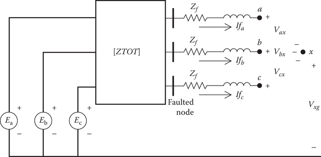
FIGURE 10.23
Thevenin equivalent circuit.

Since the matrices $[Y]$ and $[E_{a b c}]$ are known, define:

$[I P_{a b c}] = [Y] \cdot [E_{a b c}]$ (10.36)

Substituting Equation 10.19 into Equation 10.17 and rearranging results in:

$[I P_{a b c}] = [I f_{a b c}] + [Y] \cdot [V_{a b c x}] + [Y] \cdot [V_{x g}]$ (10.37)

Expanding Equation 10.37:

$\begin{matrix} [\begin{matrix} I P_{a} \\ I P_{b} \\ I P_{c} \end{matrix}] = [\begin{matrix} I f_{a} \\ I f_{b} \\ I f_{c} \end{matrix}] + [\begin{matrix} Y_{a a} & Y_{a b} & Y_{a c} \\ Y_{b a} & Y_{b b} & Y_{b c} \\ Y_{c a} & Y_{c b} & Y_{c c} \end{matrix}] \cdot [\begin{matrix} V_{a x} \\ V_{b x} \\ V_{c x} \end{matrix}] \\ + [\begin{matrix} Y_{a a} & Y_{a b} & Y_{a c} \\ Y_{b a} & Y_{b b} & Y_{b c} \\ Y_{c a} & Y_{c b} & Y_{c c} \end{matrix}] \cdot [\begin{matrix} V_{x g} \\ V_{x g} \\ V_{x g} \end{matrix}] \end{matrix}$ (10.38)

Performing the matrix operations in Equation 10.38:

$\begin{array}{l} I P_{a} = I f_{a} + (Y_{a a} \cdot V_{a x} + Y_{a b} \cdot V_{b x} + Y_{a c} \cdot V_{c x}) + Y s_{a} \cdot V_{x g} \\ I P_{b} = I f_{b} + (Y_{b a} \cdot V_{a x} + Y_{b b} \cdot V_{b x} + Y_{b c} \cdot V_{c x}) + Y s_{b} \cdot V_{x g} \\ I P_{c} = I f_{a} + (Y_{c a} \cdot V_{a x} + Y_{c b} \cdot V_{b x} + Y_{c c} \cdot V_{c x}) + Y s_{c} \cdot V_{x g} \end{array}$ (10.39)

where

$\begin{array}{l} Y s_{a} = Y_{a a} + Y_{a b} + Y_{a c} \\ Y s_{b} = Y_{b a} + Y_{b b} + Y_{b c} \\ Y s_{c} = Y_{c a} + Y_{c b} + Y_{c c} \\ or: Y s_{i} = \sum_{k = 1}^{3} Y_{i, k} \end{array}$ (10.40)

Equations 10.39 become the general equations that are used to simulate all types of short circuits. Basically, there are three equations and seven unknowns ( $I f_{a}, I f_{b}, I f_{c}, V_{a x}, V_{b x}, V_{c x}, and V_{x g}$ ). The other three variables in the equations ( $I P_{a}, I P_{b}, and I P_{c}$ ) are functions of the total impedance and the Thevenin voltages and are therefore known. In order to solve Equations 10.22, it will be necessary to specify four additional independent equations. These equations are functions of the type of fault being simulated. The additional four equations required for various types of faults are given below. These values are determined by placing short circuits in Figure 10.13 to simulate the particular type of fault. For example, a three-phase fault is simulated by placing a short circuit from node a to x, node b to x, and node c to x. That gives three voltage equations. The fourth equation comes from applying KCL at node x, which gives the sum of the fault currents to be zero.

10.2.2 Specific Short Circuits

Three-Phase Faults

$\begin{array}{l} V_{a x} = V_{b x} = V_{c x} = 0 \\ I_{a} + I_{b} + I_{c} = 0 \end{array}$ (10.41)

Three-phase-to-ground Faults

$V_{a x} = V_{b x} = V_{c x} = V_{x g} = 0$ (10.42)

Line-to-line Faults (assume i–j fault with phase k unfaulted)

$\begin{array}{l} V_{i x} = V_{j x} = 0 \\ I f_{k} = 0 \\ I f_{i} + I f_{j} = 0 \end{array}$ (10.43)

Line-to-line-to-ground Faults (assume i–j–g fault with phase k unfaulted)

$\begin{array}{l} V_{i x} = V_{j x} = 0 \\ V_{x g} = 0 \\ I_{k} = 0 \end{array}$ (10.44)

Line-to-ground Faults (assume phase k fault with phases i and j unfaulted)

$\begin{array}{l} V_{k x} = V_{x g} = 0 \\ I f_{i} = I f_{j} = 0 \end{array}$ (10.45)

Notice that Equations 10.43, 10.44, and 10.45 will allow the simulation of line-to-line faults, line-to-line-to-ground, and line-to-ground faults for all phases. There is no limitation to b–c faults for line-to-line and a–g for line-to-ground as is the case when the method of symmetrical components is employed.

A good way to solve the seven equations is to set them up in matrix form.

$[\begin{matrix} I P_{a} \\ I P_{b} \\ I P_{c} \\ 0 \\ 0 \\ 0 \\ 0 \end{matrix}] = [\begin{matrix} 1 & 0 & 0 & Y_{1, 1} & Y_{1, 2} & Y_{1, 3} & Y_{s}_{_{1}} \\ 0 & 1 & 0 & Y_{2, 1} & Y_{2, 2} & Y_{2, 3} & Y_{s}_{_{2}} \\ 0 & 0 & 1 & Y_{3, 1} & Y_{3, 2} & Y_{3, 3} & Y_{s}_{_{3}} \\ _ & _ & _ & _ & _ & _ & _ \\ _ & _ & _ & _ & _ & _ & _ \\ _ & _ & _ & _ & _ & _ & _ \\ _ & _ & _ & _ & _ & _ & _ \end{matrix}] \cdot [\begin{matrix} I f_{a} \\ I f_{b} \\ I f_{c} \\ V_{a x} \\ V_{b x} \\ V_{c x} \\ V_{x g} \end{matrix}]$ (10.46)

Equation 10.29 in condensed form:

$[I P_{s}] = [C] \cdot [X]$ (10.47)

Equation 10.47 can be solved for the unknowns in matrix [X]:

$[X] = {[C]}^{- 1} \cdot [I P_{s}]$ (10.48)

The blanks in the last four rows of the coefficient matrix in Equation 10.46 are filled in with the known variables depending upon what type of fault is to be simulated. For example, the elements in the [C] matrix simulating a three-phase fault would be:

$\begin{array}{l} C_{4, 4} = C_{5, 5} = C_{6, 6} = 1 \\ C_{7, 1} = C_{7, 2} = C_{7, 3} = 1 \end{array}$

All of the other elements in the last four rows will be set to zero.

Example 10.5

Use the system in Example 10.2, and compute the short-circuit currents for a bolted (Z_f = 0) line-to-line fault between Phases a and b at node 4.

The infinite bus balanced line-to-line voltages are 12.47 kV, which leads to balanced line-to-neutral voltages at 7.2 kV.

$[E L L_{s}] = [\begin{matrix} 12, 470 \underset{___}{/ 30} \\ 12, 470 \underset{____}{/ - 90} \\ 12, 470 \underset{____}{/ 150} \end{matrix}] V$

$[E L N_{s}] = [W] \cdot [E L L_{s}] [\begin{matrix} 7199.6 \underset{__}{/ 0} \\ 7199.6 \underset{_____}{/ - 120} \\ 7199.6 \underset{____}{/ 120} \end{matrix}] V$

The line-to-neutral Thevenin circuit voltages at node 4 are determined using Equation 8.165.

$[E t h_{4}] = [A_{t}] \cdot [E L N_{s}] = [\begin{matrix} 2400 \underset{____}{/ - 30} \\ 2400 \underset{_____}{/ - 150} \\ 2400 \underset{____}{/ 150} \end{matrix}] V$

The Thevenin equivalent impedance at the secondary terminals (node 3) of the transformer consists of the primary line impedances referred across the transformer plus the transformer impedances. Using Equation 8.165:

$[Z t h_{3}] = [A_{t}] \cdot [Z e q S_{A B C}] \cdot [d_{t}] + [Z t_{a b c}]$

$[Z t h_{3}] = [\begin{matrix} 0.0366 + j 0.1921 & - 0.0039 - j 0.0086 & - 0.0039 - j 0.0106 \\ - 0.0039 - j 0.0086 & 0.0366 + j 0.1886 & - 0.0039 - j 0.0071 \\ - 0.0039 - j 0.0106 & - 0.0039 - j 0.0071 & 0.0366 + j 0.1906 \end{matrix}] Ω$

Note that the Thevenin impedance matrix is not symmetrical. This is a result, once again, of the unequal mutual coupling between the phases of the primary line segment.

The total Thevenin impedance at node 4 is:

$[Z t h_{4}] = [Z T O T] = [Z t h_{3}] + [Z e q L_{a b c}]$

$[Z T O T] = [\begin{matrix} 0.2273 + j 0.6955 & 0.0568 + j 0.2216 & 0.0559 + j 0.1645 \\ 0.0568 + j 0.2216 & 0.2305 + j 0.6771 & 0.0575 + j 0.1860 \\ 0.0559 + j 0.1645 & 0.0575 + j 0.1860 & 0.2287 + j 0.6876 \end{matrix}] Ω$

The equivalent admittance matrix at node 4 is:

$[Y e q_{4}] = {[Z T O T]}^{- 1}$

$[Y e q_{4}] = [\begin{matrix} 0.5031 - j 1.4771 & - 0.1763 + j 0.3907 & - 0.0688 + j 0.2510 \\ - 0.1763 + j 0.3907 & 0.5501 - j 1.5280 & - 0.1148 + j 0.3133 \\ - 0.0688 + j 0.2510 & - 0.1148 + j 0.3133 & 0.4843 - j 1.4532 \end{matrix}] S$

Using Equation 10.36, the equivalent injected currents at the point of fault are:

$[I P] = [Y e q_{4}] \cdot [E t h_{4}] = [\begin{matrix} 4466.8 \underset{______}{/ - 96.3} \\ 4878.9 \underset{______}{/ 138.0} \\ 4440.9 \underset{_____}{/ 16.4} \end{matrix}] A$

The sums of each row of the equivalent admittance matrix are computed according to Equation 10.40.

$Y s_{i} = \sum_{k = 1}^{3} Y e q_{i, k} = [\begin{matrix} 0.2580 - j 0.8354 \\ 0.2590 - j 0.8240 \\ 0.3008 - j 0.8889 \end{matrix}] S$

For the a–b fault at node 4, according to Equation 10.43:

$\begin{array}{l} V_{a x} = 0 \\ V_{b x} = 0 \\ I f_{c} = 0 \\ I f_{a} + I f_{b} = 0 \end{array}$

The coefficient matrix [C] using Equation 10.46:

$[C] = [\begin{matrix} 1 & 0 & 0 & 0.5031 - j 1.4771 & - 0.1763 + j 0.3907 & - 0.0688 + 0.2510 & 0.2580 - j .8354 \\ 0 & 1 & 0 & - 0.1763 + j .3907 & 0.5501 - j 1.5280 & - 0.1148 + j .3133 & 0.2590 - j .8240 \\ 0 & 0 & 1 & - 0.0688 + j .2510 & - 0.1148 + j .3133 & 0.4843 - j 1.4532 & 0.3008 - j .8890 \\ 0 & 0 & 0 & 1 & 0 & 0 & 0 \\ 0 & 0 & 0 & 0 & 1 & 0 & 0 \\ 0 & 0 & 1 & 0 & 0 & 0 & 0 \\ 1 & 1 & 0 & 0 & 0 & 0 & 0 \end{matrix}]$

The injected current matrix is:

$[I P_{s}] = [\begin{matrix} 4466.8 \underset{______}{/ - 96.3} \\ 4878.9 \underset{______}{/ 138.0} \\ 4440.9 \underset{_____}{/ 16.4} \\ 0 \\ 0 \\ 0 \\ 0 \end{matrix}]$

The unknowns are computed by:

$[X] = {[C]}^{- 1} \cdot [I P_{s}] = [\begin{matrix} 4193.7 \underset{______}{/ - 69.7} \\ 4193.7 \underset{______}{/ 110.3} \\ 0 \\ 0 \\ 0 \\ 3646.7 \underset{_____}{/ 88.1} \\ 1220.2 \underset{______}{/ - 91.6} \end{matrix}]$

The interpretation of the results are:

$\begin{array}{l} I f_{a} = X_{1} = 4193.7 \underset{______}{/ - 69.7} \\ I f_{b} = X_{2} = 4193.7 \underset{______}{/ 110.3} \\ I f_{c} = X_{3} = 0 \\ V_{a x} = X_{4} = 0 \\ V_{b x} = X_{5} = 0 \\ V_{c x} = X_{6} = 3646.7 \underset{_____}{/ 88.1} \\ V_{x g} = X_{7} = 1220.2 \underset{_____}{/ - 91.6} \end{array}$

Using the line-to-ground voltages at node 4 and the short-circuit currents and working back to the source using the generalized matrices will check the validity of these results.

The line-to-ground voltages at node 4 are:

$[V L G_{4}] = [\begin{matrix} V_{a x} + V_{x g} \\ V_{b x} + V_{x g} \\ V_{c x} + V_{x g} \end{matrix}] = [\begin{matrix} 1220.2 \underset{______}{/ - 91.6} \\ 1220.2 \underset{______}{/ - 91.6} \\ 2426.5 \underset{_____}{/ 88.0} \end{matrix}] V$

The short-circuit currents in matrix form are:

$[I_{4}] = [I_{3}] = [\begin{matrix} 4193.7 \underset{______}{/ - 69.7} \\ 4193.7 \underset{______}{/ 110.3} \\ 0 \end{matrix}] A$

The line-to-ground voltages at node 3 are:

$[V L G_{3}] = [a_{2}] \cdot [V L G_{4}] + [b_{1}] \cdot [I_{4}] = [\begin{matrix} 1814.0 \underset{_________}{/ - 47.3} \\ 1642.1 \underset{_________}{/ - 139.2} \\ 2405.1 \underset{_________}{/ 89.7} \end{matrix}] V$

The equivalent line-to-neutral voltages and line currents at the primary terminals (node 2) of the transformer are:

$[V L N_{2}] = [a_{t}] \cdot [V L G_{3}] + [b_{t}] \cdot [I_{3}] = [\begin{matrix} 6784.3 \underset{____}{/ 0.2} \\ 7138.8 \underset{______}{/ - 118.7} \\ 7080.6 \underset{______}{/ 118.3} \end{matrix}] V$

$[I_{2}] = [d_{t}] \cdot [I_{3}] = [\begin{matrix} 1614.3 \underset{______}{/ - 69.7} \\ 807.1 \underset{______}{/ 110.3} \\ 807.1 \underset{______}{/ 110.3} \end{matrix}] A$

Finally, the equivalent line-to-neutral voltages at the infinite bus can be computed.

$[V L N_{1}] = [a_{1}] \cdot [V L N_{2}] + [b_{1}] \cdot [I_{2}] = [\begin{matrix} 7201.2 \underset{__}{/ 0} \\ 7198.2 \underset{_____}{/ - 120} \\ 7199.3 \underset{____}{/ 120} \end{matrix}] V$

The source line-to-line voltages are:

$[V L L_{1}] = [D v] \cdot [V L N_{1}] = [\begin{matrix} 12, 470 \underset{_____}{/ 30} \\ 12, 470 \underset{____}{/ - 90} \\ 12, 470 \underset{____}{/ 150} \end{matrix}]$

These are the same line-to-line voltages that were used to start the short-circuit analysis.

10.2.3 Backfeed Ground Fault Currents

The wye–delta transformer bank is the most common transformer connection used to serve three-phase loads or a combination of a single-phase lighting load and a three-phase load. With this connection, a decision has to be made as to whether or not to ground the neutral of the primary wye connection. The neutral can be directly connected to the ground or grounded through a resistor or left floating (ungrounded wye–delta). When the neutral is grounded, the transformer bank becomes a grounding bank that provides a path for zero sequence fault currents. In particular, the grounded connection will provide a path for a line-to-ground fault current (backfeed current) for a fault upstream from the transformer bank. A method for the analysis of the upstream fault currents will be presented [6].

10.2.3.1 One Downstream Transformer Bank

A simple system consisting of one downstream grounded wye–delta transformer bank is shown in Figure 10.24.

In Figure 10.24, the substation transformer is connected to a high-voltage equivalent source consisting of a three-phase voltage source and an equivalent impedance matrix. The equivalent source and substation transformer bank combination can be represented as shown in Figure 10.25.

In Chapter 8, it was shown that the combination of the equivalent source and substation transformer could be reduced to a Thevenin equivalent circuit as shown in Figure 10.26.

images

FIGURE 10.24
Simple system.

images

FIGURE 10.25
Equivalent source and substation transformer.

images

FIGURE 10.26
Thevenin equivalent circuit.

The Thevenin equivalent voltages and impedance matrix are given by:

$\begin{array}{l} [E t h] = [A_{t}] \cdot [E L G_{123}] \\ [Z t h_{A B C}] = [A_{t}] \cdot [Z s y s_{123}] \cdot [d_{t}] + [B_{t}] \\ where for the delta-grounded wye transformer: \\ n_{t} = \frac{k V L L_{_{primary}}}{k V L N_{_{secondary}}} \\ [A_{t}] = \frac{1}{n_{t}} \cdot [\begin{matrix} 1 & 0 & - 1 \\ - 1 & 1 & 0 \\ 0 & - 1 & 1 \end{matrix}] \\ [B_{t}] = [\begin{matrix} Z t_{_{a}} & 0 & 0 \\ 0 & Z t_{b} & 0 \\ 0 & 0 & Z t_{_{c}} \end{matrix}] \\ [d_{t}] = \frac{1}{n_{t}} \cdot [\begin{matrix} 1 & - 1 & 0 \\ 0 & 1 & - 1 \\ - 1 & 0 & 1 \end{matrix}] \\ [Z sys_{_{123}}] = [\begin{matrix} Z l_{_{1, 1}} & Z l_{_{1, 2}} & Z l_{_{1, 3}} \\ Z l_{_{2, 1}} & Z l_{_{2, 2}} & Z l_{_{2, 3}} \\ Z l_{_{3, 1}} & Z l_{_{3, 2}} & Z l_{_{3, 3}} \end{matrix}] \end{array}$ (10.49)

Applying the Thevenin equivalent circuit, Figure 10.24 is modified to that of Figure 10.27.

In Figure 10.27, the equivalent impedance matrix is:

$[Z e q] = [Z t h_{A B C}] + [Z 12_{A B C}]$ (10.50)

A question that comes up when a wye–delta transformer bank is to be installed is whether the neutral should be grounded. If the neutral is to be grounded, it can either be a direct ground or be grounded through a resistance. The other option is to just leave the neutral floating. Figure 10.28 shows the three-phase circuit for the modified simple system in Figure 10.27 when a line-to-ground fault has occurred at node 2 in Figure 10.27. Note the question mark on grounding of the neutral.

images

FIGURE 10.27
Modified simple system.

images

FIGURE 10.28
Three-phase circuit with floating transformer neutral.

For future reference, the source voltages are $[E_{s}_{_{A B C}}] = [E_{t h}]$ . When the neutral is left floating in Figure 10.28, there is no path for the currents to flow from the transformer back to the fault. In this case, the only short-circuit current will be from the substation to the faulted node.

Figure 10.29 represents the transformer bank grounded neutral through a resistance.

images

FIGURE 10.29
Three-phase circuit with grounded transformer neutral.

Before getting into the derivation of the computation of the short-circuit currents in Figure 10.29, it is important to do a visual analysis of the circuit. The most important observation is that there is a path for the current $I t_{_{A}}$ to flow from the phase A transformer through the fault and back to the neutral through the grounding resistance (Z_g). Note that this resistance can be set to zero for the direct grounding of the neutral. Because $I t_{_{A}}$ flows, there must be a current in the delta transformer secondary. This current is given by:

$I_{a b} = n_{t} \cdot I_{t}_{_{A}}$ (10.51)

Because the line currents out of the delta are zero, then all of the currents flowing in the delta must be equal.

$I_{a b} = I_{b c} = I_{c a} = n_{t} \cdot I_{t}_{_{A}}$ (10.52)

Because the delta currents are equal, define the currents out of the transformer:

$I t_{A} = I t_{B} = I t_{C} = I t$ (10.53)

The sum of the line-to-line secondary voltages must add to zero:

$V_{a b} + V_{b c} + V_{c a} = 0$ (10.54)

10.2.3.2 Complete Three-Phase Circuit Analysis

A method to calculate the short-circuit currents is to apply basic circuit and transformer analysis to determine all voltages and currents. A three-phase circuit showing an A–G fault at node 2 is shown in Figure 10.29. There are 28 unknowns, which will require 28 independent equations. Without going into detail, the 28 equations are:

13 KVL
6 basic transformer primary/secondary
5 KCL
4 unique to type of fault

The 28 independent equations will be reduced to 8 independent equations that will compute the voltages and currents in the fault and the backfeed current from the transformer bank. All other system voltages and currents can be computed by knowing these eight variables.

In Figure 10.30, a node X has been installed to represent the fault at node 2. With the node X, there are four voltages defined as $V f_{A X}, V f_{B X}, V f_{C X}, V f_{X G}$ and three fault currents defined as $I f_{A}, I f_{B}, I f_{C}$ . The different types of faults are modeled by setting the appropriate voltages and currents to zero. For example, for an A–G fault, the following conditions are set:

images

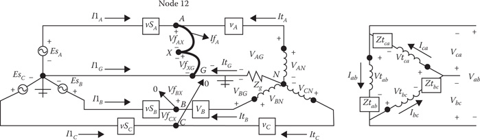
FIGURE 10.30
Three-phase circuit with AG fault.

$\begin{array}{l} V f_{A X} = 0 \\ V f_{X G} = 0 \\ I f_{B} = 0 \\ I f_{C} = 0 \end{array}$ (10.55)

In Figure 10.30, three loop equations can be written between the source and the faulted node.

$\begin{array}{l} E s_{A} = V f_{A X} + V f_{X G} + Z e q_{1,1} \cdot I 1_{A} + Z e q_{1,2} \cdot I 1_{B} + Z e q_{1,3} \cdot I 1_{C} \\ E s_{B} = V f_{B X} + V f_{X G} + Z e q_{2,1} \cdot I 1_{A} + Z e q_{2,2} \cdot I 1_{B} + Z e q_{2,3} \cdot I 1_{C} \\ E s_{C} = V f_{C X} + V f_{X G} + Z e q_{3,1} \cdot I 1_{A} + Z e q_{3,2} \cdot I 1_{B} + Z e q_{3,3} \cdot I 1_{C} \end{array}$ (10.56)

KCL can be applied at the faulted node point:

$\begin{array}{l} I 1_{A} = I f_{A} - I t \\ I 1_{B} = I f_{B} - I t \\ I 1_{C} = I f_{C} - I t \end{array}$ (10.57)

Substitute Equation 10.57 into Equation 10.56:

$\begin{array}{l} E s_{A} = V f_{A X} + V f_{X G} + Z e q_{1,1} \cdot I f_{A} + Z e q_{1,2} \cdot I f_{B} + Z e q_{1,3} \cdot I f_{C} - Z x_{1} \cdot I t \\ E s_{B} = V f_{B X} + V f_{X G} + Z e q_{2,1} \cdot I f_{A} + Z e q_{2,2} \cdot I f_{B} + Z e q_{2,3} \cdot I f_{C} - Z x_{2} \cdot I t \\ E s_{C} = V f_{C X} + V f_{X G} + Z e q_{3,1} \cdot I f_{A} + Z e q_{3,2} \cdot I f_{B} + Z e q_{3,3} \cdot I f_{C} - Z x_{3} \cdot I t \\ where for \\ i = 1, 2, 3: Z x_{i} = \sum_{k = 1}^{3} Z eq_{_{i, k}} \end{array}$ (10.58)

The line-to-ground voltages at the transformer primary terminals are:

$\begin{array}{l} V_{A G} = V f_{A X} + V f_{X G} + (Z 23_{11} + Z 23_{12} + Z 23_{13}) \cdot I t \\ V_{B G} = V f_{B X} + V f_{X G} + (Z 23_{21} + Z 23_{22} + Z 23_{23}) \cdot I t \\ V_{C G} = V f_{C X} + V f_{X G} + (Z 23_{31} + Z 23_{32} + Z 23_{33}) \cdot I t \end{array}$

$\begin{array}{l} V_{A G} = V f_{A X} + V f_{X G} + Z y_{1} \cdot I t \\ V_{B G} = V f_{B X} + V f_{X G} + Z y_{2} \cdot I t \\ V_{C G} = V f_{C X} + V f_{X G} + Z y_{2} \cdot I t \end{array}$ (10.59)

The line-to-neutral ideal transformer voltages are:

$\begin{array}{l} V_{A N} = V_{A G} + 3 \cdot Z_{g} \cdot I_{t} \\ V_{A N} = V_{B G} + 3 \cdot Z_{g} \cdot I_{t} \\ V_{A N} = V_{C G} + 3 \cdot Z_{g} \cdot I_{t} \end{array}$ (10.60)

Substitute Equation 10.59 into Equation 10.60:

$\begin{array}{l} V_{A N} = V_{A G} + 3 \cdot Z_{g} \cdot I t = V f_{A X} + V f_{X G} + (Z y_{1} + 3 \cdot Z_{g}) \cdot I t \\ V_{B N} = V_{B G} + 3 \cdot Z_{g} \cdot I t = V f_{B X} + V f_{X G} + (Z y_{2} + 3 \cdot Z_{g}) \cdot I t \\ V_{C N} = V_{C G} + 3 \cdot Z_{g} \cdot I t = V f_{C X} + V f_{X G} + (Z y_{3} + 3 \cdot Z_{g}) \cdot I t \end{array}$ (10.61)

From the currents flowing in the delta secondary are:

$\begin{array}{l} I_{a b} = I_{b c} = I_{c a} = n_{t} \cdot I_{t}_{_{A}} \\ I_{a b} = I_{b c} = I_{c a} = n_{t} \cdot I_{t} \\ since: I_{t}_{_{A}} = I_{t} \end{array}$ (10.62)

The line-to-line secondary voltages are:

$\begin{array}{l} V_{a b} = V t_{a b} + Z t_{a b} \cdot I_{a b} \\ V_{b c} = V t_{b c} + Z t_{b c} \cdot I_{b c} \\ V_{c a} = V t_{c a} + Z t_{c a} \cdot I_{c a} \end{array}$ (10.63)

In Equation 10.63:

$\begin{array}{l} V t_{a b} = \frac{1}{n_{t}} \cdot V_{A N} \\ V t_{b c} = \frac{1}{n_{t}} \cdot V_{B N} \\ V t_{c a} = \frac{1}{n_{t}} \cdot V_{C N} \\ I_{a b} = I_{b c} = I_{c a} = n_{t} \cdot I t \end{array}$ (10.64)

Substitute Equation 10.64 into Equation 10.63:

$\begin{array}{l} V_{a b} = \frac{1}{n_{t}} \cdot V_{A N} + Z t_{a b} \cdot n_{t} \cdot I t \\ V_{b c} = \frac{1}{n_{t}} \cdot V_{B N} + Z t_{b c} \cdot n_{t} \cdot I t \\ V_{c a} = \frac{1}{n_{t}} \cdot V_{C N} + Z t_{c a} \cdot n_{t} \cdot I t \\ but: \\ V_{a b} + V_{b c} + V_{c a} = 0 \\ therefore: \\ 0 = \frac{1}{n_{t}} \cdot (V_{A N} + V_{B N} + V_{C N}) + n_{t} \cdot Z t_{_{sum}} \cdot I t \\ where \\ Z t_{_{sum}} = Z t_{_{a b}} + Z t_{_{b c}} + Z t_{_{c a}} \end{array}$ (10.65)

Substitute Equation 10.61 into Equation 10.65:

$\begin{array}{l} 0 = \frac{1}{n_{t}} \cdot (V_{A N} + V_{B N} + V_{C N}) + n_{t} \cdot Z t_{s u m} \cdot I t \\ V_{A N} = V f_{A X} + V f_{X G} + (Z y_{1} + 3 \cdot Z_{g}) \cdot I t \\ V_{B N} = V f_{B X} + V f_{X G} + (Z y_{2} + 3 \cdot Z_{g}) \cdot I t \\ V_{C N} = V f_{C X} + V f_{X G} + (Z y_{3} + 3 \cdot Z_{g}) \cdot I t \\ 0 = \frac{1}{n_{t}} \cdot ((V f_{A X} + V f_{B X} + V f_{C X} + 3 \cdot V f_{X G}) + Z y_{s u m} + 9 \cdot Z_{g}) \cdot I t + n_{t} \cdot Z t_{s u m} \cdot I t \\ 0 = \frac{1}{n_{t}} \cdot (V f_{A X} + V f_{B X} + V f_{C X} + 3 \cdot V f_{X G}) + \frac{1}{n_{t}} \cdot (Z y_{s u m} + n_{t}^{2} \cdot Z t_{s u m} + 9 \cdot Z_{g}) \cdot I t \\ 0 = \frac{1}{n_{t}} \cdot (V f_{A X} + V f_{B X} + V f_{C X} + 3 \cdot V f_{X G}) + Z_{t o t a l} \cdot I t \end{array}$ (10.66)

where

$Z_{t o t a l} = \frac{1}{n_{t}} \cdot (Z y_{s u m} + n_{t}^{2} \cdot Z t_{s u m} + 9 \cdot Z_{g})$

Combining Equations 10.58 and 10.66 gives four equations with eight unknowns:

$\begin{array}{l} E_{s}_{_{A}} = V_{f}_{_{A X}} + V_{f}_{_{X G}} + Z_{eq}_{_{1, 1}} \cdot I_{f}_{_{A}} + Z_{eq}_{_{1, 2}} \cdot I_{f}_{_{B}} + Z_{eq}_{_{1, 3}} \cdot I_{f}_{_{C}} - Z x_{1} \cdot I_{t} \\ E_{s}_{_{B}} = V_{f}_{B X} + V_{f}_{_{X G}} + Z_{eq}_{_{2, 1}} \cdot I_{f}_{_{A}} + Z_{eq}_{_{2, 2}} \cdot I_{f}_{_{B}} + Z_{eq}_{_{2, 3}} \cdot I_{f}_{_{C}} - Z x_{2} \cdot I_{t} \\ E_{s}_{_{C}} = V_{f}_{_{C X}} + V_{f}_{_{X G}} + Z_{eq}_{_{3, 1}} \cdot I_{f}_{_{A}} + Z_{eq}_{_{3, 2}} \cdot I_{f}_{_{B}} + Z_{eq}_{_{3, 3}} \cdot I_{f}_{_{C}} - Z x_{3} \cdot I_{t} \\ 0 = \frac{1}{n_{t}} \cdot (V_{f}_{_{A X}} + V_{f}_{_{B X}} + V_{f}_{_{C X}} + 3 \cdot V_{f}_{_{X G}}) + Z_{total} \cdot I_{t} \end{array}$ (10.67)

where

$\begin{array}{l} Z_{t o t a l} = \frac{1}{n_{t}} \cdot (Z y_{s u m} + Z t_{s u m} + 9 \cdot Z_{g}) \\ Z y_{s u m} = Z y_{1} + Z y_{2} + Z y_{3} \\ Z t_{s u m} = Z t_{a b} + Z t_{b c} + Z t_{c a} \end{array}$

Equation 10.67 gives four independent equations. The final four independent equations are unique for the type of fault to be modeled. The four equations that model each of the various types of faults are defined in Equations 10.41 to 10.45.

A general matrix equation for modeling a B–C–G fault is shown in the forthcoming. The first four rows in the coefficient matrix [C] come from Equation 10.69, and the last four rows are for the B–C–G fault as specified in Section 10.2.2.

$\begin{array}{l} [\begin{matrix} E s_{A} \\ E s_{B} \\ E s_{C} \\ 0 \\ 0 \\ 0 \\ 0 \\ 0 \end{matrix}] = [\begin{matrix} Z e q_{1,1} & Z e q_{1,2} & Z e q_{1,3} & - Z x_{1} & 1 & 0 & 0 & 1 \\ Z e q_{2,1} & Z e q_{2,2} & Z e q_{2,3} & - Z x_{2} & 0 & 1 & 0 & 1 \\ Z e q_{3,1} & Z e q_{3,2} & Z e q_{3,3} & - Z x_{3} & 0 & 0 & 1 & 1 \\ 0 & 0 & 0 & Z_{t o t a l} & \frac{1}{n_{t}} & \frac{1}{n_{t}} & \frac{1}{n_{t}} & \frac{3}{n_{t}} \\ 1 & 0 & 0 & 0 & 0 & 0 & 0 & 0 \\ 0 & 0 & 0 & 0 & 0 & 1 & 0 & 0 \\ 0 & 0 & 0 & 0 & 0 & 0 & 1 & 0 \\ 0 & 0 & 0 & 0 & 0 & 0 & 0 & 1 \end{matrix}] \cdot [\begin{matrix} I f_{A} \\ I f_{B} \\ I f_{C} \\ I t \\ V f_{A X} \\ V f_{B X} \\ V f_{C X} \\ V f_{X G} \end{matrix}] \\ [E x] = [C] \cdot [X] \end{array}$ (10.68)

Example 10.6

The system in Figure 10.29 is to be analyzed for a B–C–G fault at node 2. The given information for the system is as follows:

Equivalent system:

$[E L L_{s y s}] = [\begin{matrix} 230, 000 \underset{___}{/ 60} \\ 230, 000 \underset{____}{/ - 60} \\ 230, 000 \underset{____}{/ 180} \end{matrix}] [E L N_{_{sys}}] = [W] \cdot [E L L_{_{sys}}] = [\begin{matrix} 132, 790.6 \underset{___}{/ 30} \\ 132, 790.6 \underset{____}{/ - 90} \\ 132, 790.6 \underset{____}{/ 150} \end{matrix}] V$

$\begin{array}{l} Line length = 200 miles \\ [Z sys_{_{123}}] = [\begin{matrix} 88.1693 + j 226.9581 & 25.6647 + j 90.9260 & 25.6647 + j 71.3971 \\ 25.6647 + j 90.9260 & 87.7213 + j 235.6914 & 24.5213 + j 78.2847 \\ 25.6647 + j 71.3971 & 24.5213 + j 78.2847 & 85.7213 + j 235.6814 \end{matrix}] Ω \end{array}$

Substation transformer:

$\begin{array}{l} k V A = 2500 k V L L_{p r i} = 230 k V L L_{s e c} = 12.47 Z_{s u b} = 0.005 + j 0.06 per-unit \\ Z b a s e_{s e c} = \frac{k V L L_{s e c}^{2} \cdot 1000}{k V A} = 62.2004 \\ Z t = Z t_{s u b} \cdot Z b a s e_{s e c} = 0.311 + j 3.732 \\ [Z s u b_{ABC}] = [\begin{matrix} 0.311 + j 3.732 & 0 & 0 \\ 0 & 0.311 + j 3.732 & 0 \\ 0 & 0 & 0.311 + j 3.732 \end{matrix}] \end{array}$

Compute substation transformer matrices:

$\begin{array}{l} k V L N_{s e c} = \frac{k V L L_{s e c}}{\sqrt{3}} = 7.1996 \\ n_{t} = \frac{k V L L_{p r i}}{k V L N_{s e c}} = 31.9464 \\ [A_{t}] = \frac{1}{n_{t}} \cdot [\begin{matrix} 1 & 0 & - 1 \\ - 1 & 1 & 0 \\ 0 & - 1 & 1 \end{matrix}] \\ [B_{t}] = [Z s u b_{ABC}] \\ [d_{t}] = \frac{1}{n_{t}} \cdot [\begin{matrix} 1 & - 1 & 0 \\ 0 & 1 & - 1 \\ - 1 & 0 & 1 \end{matrix}] \end{array}$

Compute substation transformer Thevenin equivalent circuit relative to secondary (Chapter 8, Section 8.12):

$\begin{array}{l} [E_{t h}] = [A_{t}] \cdot [E L N_{s y s}] = [\begin{matrix} 7199.5579 \underline{/ 0} \\ 7199.5579 \underline{/ - 120} \\ 7199.5579 \underline{/ 120} \end{matrix}] \\ [Z t h_{A B C}] = [A_{t}] \cdot [Z s y s_{123}] \cdot [d_{t}] + [B_{t}] \\ [Z t h_{A B C}] = [\begin{matrix} 0.4311 + j 4.40454 & - 0.0601 - j 0.1400 & - 0.0600 - j 0.1734 \\ - 0.0601 - j 0.1400 & 0.4311 + j 4.0071 & - 0.0600 - j 0.1351 \\ - 0.0600 - j 0.1734 & - 0.0600 - j 0.1351 & 0.4309 + j 4.0405 \end{matrix}] \end{array}$

Given distribution line impedance matrices as follows:

$\begin{array}{l} [Z 12_{A B C}] = [\begin{matrix} 0.9151 + j 2.1561 & 0.3119 + j 1.0033 & 0.3070 + j 0.7699 \\ 0.3119 + j 1.0033 & 0.9333 + j 2.0963 & 0.3160 + j 0.8473 \\ 0.3070 + j 0.7699 & 0.3160 + j 0.8473 & 0.9229 + j 2.1301 \end{matrix}] \\ [Z 23_{A B C}] = [\begin{matrix} 0.4576 + j 1.0780 & 0.1559 + j 0.5017 & 0.1535 + j 0.3849 \\ 0.1559 + j 0.5017 & 0.4666 + j 1.0482 & 0.1580 + j 0.4236 \\ 0.1535 + j 0.3849 & 0.1580 + j 0.4236 & 0.4615 + j 1.0651 \end{matrix}] Ω \end{array}$

Grounded wye–delta transformer data:

$\begin{array}{l} k V A_{1} = 50 k V A_{2} = 100 k V A_{3} = 50 \\ Z t {_{_{pu}}}_{_{_{1}}} = 0.011 + j 0.018 Z t {_{_{pu}}}_{_{_{2}}} = 0.01 + j 0.021 Z t {_{_{pu}}}_{_{_{3}}} = 0.011 + j 0.018 \\ k V_{L N}_{_{pri}} = 7.2 k V_{L L}_{_{\sec}} = 0.48 \\ n_{t} = \frac{k V_{L N}_{_{pri}}}{k V_{L L}_{_{\sec}}} = 15 \\ For i = 1, 2, 3 Z_{D} {_{_{base}}}_{_{_{i}}} = \frac{k V_{L L} {_{_{l o}}}^{2} \cdot 1000}{k V A_{i}} = [\begin{matrix} 4.608 \\ 2.304 \\ 4.608 \end{matrix}] \\ Z t {_{_{del}}}_{_{_{i}}} = Z t {_{_{pu}}}_{_{_{i}}} \cdot Z_{D} {_{_{base}}}_{_{_{i}}} = [\begin{matrix} 0.0507 + j 0.0829 \\ 0.0230 + j 0.0484 \\ 0.0507 + j 0.0829 \end{matrix}] \\ Z t_{_{a b}} = Z t {_{_{del}}}_{_{_{1}}} Z t_{_{b c}} = Z_{t} {_{_{del}}}_{_{_{2}}} Z_{t}_{_{c a}} = Z_{t} {_{_{del}}}_{_{3}} \\ Grounding resistance: Z_{g} = 5 Ω \end{array}$

Compute impedance terms for Equation 10.50:

$\begin{array}{l} [Z e q] = [Z t h_{A B C}] + [Z 12_{A B C}] \\ [Z e q] = [\begin{matrix} 1.3462 + j 6.2015 & 0.2518 + j 0.8633 & 0.2470 + j 0.5965 \\ 0.2518 + j 0.8633 & 1.3643 + j 6.1035 & 0.2560 + j 0.7122 \\ 0.2470 + j 0.5965 & 0.2560 + j 0.7122 & 1.3539 + j 6.1706 \end{matrix}] \\ For i = 1,2,3 \\ [Z x_{i}] = \sum_{k = 1}^{3} Z e q_{i, k} = [\begin{matrix} 1.8450 + j 76613 \\ 1.8722 + j 7.6790 \\ 1.8569 + j 7.4793 \end{matrix}] \\ [Z y_{i}] = \sum_{k = 1}^{3} Z 23_{A B C_{i, k}} = [\begin{matrix} 0.7670 + j 1.9646 \\ 0.7806 + j 1.9735 \\ 0.7730 + j 1.8736 \end{matrix}] \\ Z y_{s u m} = \sum_{k = 1}^{3} Z y_{k} = 2.3205 + j 5.8118 \\ Z t_{s u m} = Z t_{a b} + Z t_{b c} + Z t_{c a} = 0.1244 + j 0.2143 \\ Z_{t o t a l} = \frac{1}{n_{t}} \cdot (Z y_{s u m} + n_{t}^{2} \cdot Z t_{s u m} + 9 \cdot Z_{g}) = 5.0209 + j 3.6015 \end{array}$

Using the Thevenin source voltages and the numerical values from above, create the Equation 10.68 matrices for the B–C–G fault at node 2. Remember that the last four rows of the [C] matrix represent the type of fault as specified in Section 10.2.2.

$[E_{x}] = [\begin{matrix} 7199.5579 \underset{__}{/ 0} \\ 7199.5579 \underset{_____}{/ - 120} \\ 7199.5579 \underset{____}{/ 120} \\ 0 \\ 0 \\ 0 \\ 0 \\ 0 \end{matrix}]$

$[C] = [\begin{matrix} 1.3462 + j 6.2015 & 0.2518 + j 0.8633 & 0.2470 + j 0.5965 & - 1.8450 - 7.6613 & 1 & 0 & 0 & 1 \\ 0.2518 + j 0.8633 & 1.3643 + j 6.1035 & 0.2560 + j 0.7122 & - 1.8722 - j 7.6790 & 0 & 1 & 0 & 1 \\ 0.2470 + j 0.5965 & 0.2560 + j 0.7122 & 1.3539 + j 6.1706 & - 1.8569 - j 7.4793 & 0 & 0 & 1 & 1 \\ 0 & 0 & 0 & 5.0209 + j 3.6015 & 0.0667 & 0.0667 & 0.0667 & 0.2 \\ 1 & 0 & 0 & 0 & 0 & 0 & 0 & 0 \\ 0 & 0 & 0 & 0 & 0 & 1 & 0 & 0 \\ 0 & 0 & 0 & 0 & 0 & 0 & 1 & 0 \\ 0 & 0 & 0 & 0 & 0 & 0 & 0 & 1 \end{matrix}]$

Solve for the unknown matrix [X]:

$[X] = {[C]}^{- 1} \cdot [E_{x}]$

The computed short-circuit currents are:

$\begin{array}{l} [\begin{matrix} I f_{A} \\ I f_{B} \\ I f_{C} \end{matrix}] = [\begin{matrix} X_{1} \\ X_{2} \\ X_{3} \end{matrix}] = [\begin{matrix} 0 \\ 1342.2 \underset{______}{/ 165.84} \\ 1194.6 \underset{______}{/ 40.15} \end{matrix}] \\ I t = X_{4} = 81.5 \underset{_______}{/ 143.53} \\ For i = 1, 2, 3 \\ [\begin{matrix} I 1_{A} \\ I 1_{B} \\ I 1_{C} \end{matrix}] = [\begin{matrix} I f_{A} \\ I f_{B} \\ I f_{C} \end{matrix}] - [\begin{matrix} I t \\ I t \\ I t \end{matrix}] = [\begin{matrix} 81.5 \underset{_______}{/ - 36.46} \\ 1267.2 \underset{_______}{/ 167.24} \\ 1216.09 \underset{______}{/ 36.41} \end{matrix}] \end{array}$

Note from above that each of the distribution transformer primary windings has a short-circuit current of 81.5 A flowing. The rated currents for the three transformers are:

$I r a t e d_{i} = \frac{k V A_{i}}{k V L N_{h i}} = [\begin{matrix} 6.94 \\ 13.89 \\ 6.94 \end{matrix}] A$

The percentage overrated current for the transformers are:

$I o v e r_{_{i}} = \frac{I t}{I h i_{i}} \cdot 100 = [\begin{matrix} 1173.6 \\ 586.8 \\ 1173.6 \end{matrix}] %$

Obviously, the fuses on the distribution transformers are going to blow because of the backfeed current.

This method of analysis for a grounded wye–delta bank with a ground resistance can be used to simulate an ungrounded wye–delta bank by setting the grounding resistance to a very large value. For example, use a grounding resistance of 99,999.

$\begin{array}{l} Z_{g} = 99, 999 \\ [I f_{_{A B C}}] = [\begin{matrix} 0 \\ 1257.4 \underset{______}{/ 167.5} \\ 1217.0 \underset{_____}{/ 36.1} \end{matrix}] \\ I_{t} = 0 \\ [I_{A B C}] = [\begin{matrix} 0 \\ 1257.4 \underset{______}{/ 167.5} \\ 1217.0 \underset{_____}{/ 36.1} \end{matrix}] \end{array}$

Note that for this case, the backfeed current from the transformer bank is zero.

10.2.3.3 Backfeed Currents Summary

When a wye–delta transformer connection is used, the basic question is whether the neutral should be grounded. In this section, a method of analyzing a simple system was developed for analysis and then demonstrated with an example. It can b e concluded that there is a very significant backfeed current when the neutral is grounded. The backfeed current is in the range of 1000% of the rated transformer currents; so the transformer fuses will blow for the upstream fault. It was also demonstrated that if the grounding resistance is set to a very large value, the backfeed current will be zero, thus simulating an ungrounded wye–delta transformer bank connection. The final conclusion is that the neutral should never be grounded either directly or through a grounding resistance.

10.3 Summary

This chapter has demonstrated the application of the element models that are used in the power-flow analysis and short-circuit analysis of a distribution feeder. The modified ladder iterative technique was used for the power-flow analysis. For a simple radial feeder with no laterals, the examples demonstrated that only the forward and backward sweeps were changed by adding the sweep equations for the new elements. A feeder with laterals and sublaterals will require the ladder forward and backward sweep for each lateral and sublateral. In some cases, there is a need to model a feeder with a limited number of loops. A loop-flow method of modifying the ladder technique was developed, and an example was developed to demonstrate the loop-flow method.

For the short-circuit analysis of a feeder, using the symmetrical component analysis will not work because not all possible short circuits can be modeled. Rather, a method in the phase domain for the computation of any type of short circuit was developed and demonstrated.

The backfeed short-circuit currents due to a grounded wye–delta transformer bank were developed and demonstrated by way of an example. The final idea is to demonstrate that a grounded wye–delta transformer bank should never be used.

The examples in this chapter have been very long and should be used as a learning tool. Many of the interesting operating characteristics of a feeder can only be demonstrated through numerical examples. The examples were designed to illustrate some of these characteristics.

Armed with a computer program using the models and techniques of this text provides the engineer with a powerful tool for solving present-day problems and long-range planning studies.

Problems

The power-flow problems in this set require the application of the modified ladder technique. Students are encouraged to write their own computer programs to solve the problems.

The first six problems of this set will be based upon the system in Figure 10.31.

images

FIGURE 10.31
Wye homework system.

The substation transformer is connected to an infinite bus with balanced three-phase voltages of 69 kV. The substation transformer is rated:

5000 kVA, 69 kV delta–4.16 grounded wye, Z = 1.5 + j8.0%

The phase impedance matrix for a four-wire wye line is:

$[z_{4-wire}] = [\begin{matrix} 0.4576 + j 1.0780 & 0.1560 + j 0.5017 & 0.1535 + j 0.3849 \\ 0.1560 + j 0.5017 & 0.4666 + j 1.0482 & 0.1580 + j 0.4236 \\ 0.1535 + j 0.3849 & 0.1580 + j 0.4236 & 0.4615 + j 1.0651 \end{matrix}] Ω /mile$

The secondary voltages of the infinite bus are balanced and being held at 69 kV for all power-flow problems.

The four-wire wye feeder is 0.75 miles long. An unbalanced wye-connected load is located at node 3 and has the following values:

Phase a: 750 kVA at 0.85 lagging power factor
Phase b: 500 kVA at 0.90 lagging power factor
Phase c: 850 kVA at 0.95 lagging power factor

The load at node 4 is zero initially.

10.1 For the system as described earlier and assuming that the regulators are in the neutral position:

Determine the forward and backward sweep matrices for the substation transformer and the line segment.
Use the modified ladder technique to determine the line-to-ground voltages at node 3. Use a tolerance of 0.0001 per-unit. Give the voltages in actual values in volts and on a 120-V base.

10.2 Three Type B step-voltage regulators are installed in a wye connection at the substation in order to hold the load voltages (node 3) at a voltage level of 121 V and a bandwidth of 2 V.

Compute the actual equivalent line impedance between nodes 2 and 3.
Use a potential transformer ratio of 2400–120 V and a current transformer ratio of 500:5 A. Determine the R and X compensator settings calibrated in volts and ohms. The settings must be the same for all three regulators.
For the load conditions in Problem 10.1 and with the regulators in the neutral position, compute the voltages across the voltage relays in the compensator circuits.
Determine the appropriate tap settings for the three regulators to hold the node 3 voltages at 121 V in a bandwidth of 2 V.
With the regulator taps set, compute the actual load voltages on a 120-V base.

10.3 A wye-connected three-phase shunt capacitor bank of 300 kvar per phase is installed at node 3. With the regulator compensator settings from Problem 10.2, determine:

The new tap settings for the three regulators
The voltages at the load on a 120-V base
The voltages across the relays in the compensator circuits

10.4 The load at node 4 is served through an ungrounded wye–delta transformer bank. The load is connected in delta with the following values:

Phase a–b: 400 kVA at 0.9 factor power factor
Phase b–c: 150 kVA at 0.8 lagging power factor
Phase c–a: 150 kVA at 0.8 lagging power factor

The three single-phase transformers are rated as:

“Lighting transformer”: 500 kVA, 2400–240 V, Z = 0.9 + j3.0%
“Power transformers”: 167 kVA, 2400–240 V, Z = 1.0 + j1.6%

Use the original loads and the shunt capacitor bank at node 3 and this new load at node 4 and determine:

The voltages on 120 V base at node 3 assuming the regulators are in the neutral position
The voltages on 120 V base at node 4 assuming the regulators are in the neutral position
The new tap settings for the three regulators
The node 3 and node 4 voltages on 120 V base after the regulators have changed tap positions

10.5 Under short-circuit conditions, the infinite bus voltage is the only voltage that is constant. The voltage regulators in the substation are in the neutral position. Determine the short-circuit currents and voltages at nodes 1, 2, and 3 for the following short circuits at node 3.

Three-phase to ground
Phase b to ground
Line-to-line fault on Phases a–c

10.6 A line-to-line fault occurs at node 4. Determine the currents in the fault and on the line segment between nodes 2 and 3. Determine the voltages at nodes 1, 2, 3, and 4.

10.7 A three-wire delta line of length 0.75 miles is serving an unbalanced delta load of:

Phase a–b: 600 kVA, 0.9 lagging power factor
Phase b–c: 800 kVA, 0.8 lagging power factor
Phase c–a: 500 kVA, 0.95 lagging power factor

The phase impedance matrix for the line is:

$[z_{3-wire}] = [\begin{matrix} 0.4013 + j 1.4133 & 0.0953 + j 0.8515 & 0.0953 + j 0.7802 \\ 0.0953 + j 0.8515 & 0.4013 + j 1.4133 & 0.0953 + j 0.7266 \\ 0.0953 + j 0.7802 & 0.0953 + j 0.7266 & 0.4013 + j 1.4133 \end{matrix}] Ω /mile$

The line is connected to a constant balanced voltage source of 4.8 kV line-to-line. Determine the load voltages on a-120 V base.

10.8 Add two Type B step-voltage regulators in an open-delta connection using phases A–B and B–C to the system in Problem 10.7. The regulator should be set to hold 121 ± 1 V. Determine the R and X settings and the final tap settings. For the open-delta connection, the R and X settings will be different on the two regulators.

10.9 The three-wire line of Problem 10.7 is connected to a substation transformer connected delta–delta. The substation transformer is connected to a 69-kV infinite bus and is rated:

10,000 kVA, 69 kV delta–4.8 kV delta, Z = 1.6 + j7.8%

Determine the short-circuit currents and substation transformer secondary voltages for the following short circuits at the end of the line:

Three-phase
Line-to-line between Phases a–b

10.10 Two three-phase systems are shown in Figure 10.32.

images

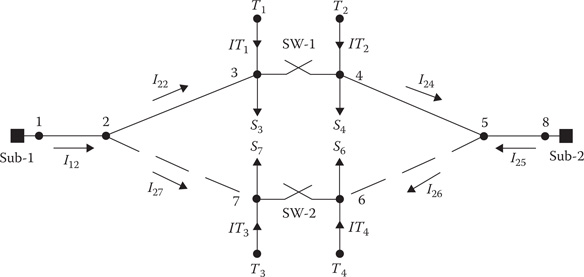
FIGURE 10.32
Loop-flow system.

In Figure 10.32, the solid lines represent three-phase lines, while the dashed lines represent phase C single-phase lines. The phase conductors are 336,400 26/7 ACSR, and the neutral conductor is 1/0 ACSR. The impedance matrices are:

Three-phase lines:

$[z 3] = [\begin{matrix} 0.5396 + j 1.0978 & 0.1916 + j 0.5475 & 0.1942 + j 0.4705 \\ 0.1916 + j 0.5475 & 0.5279 + j 1.1233 & 0.1884 + j 0.4296 \\ 0.1942 + j 0.4705 & 0.1884 + j 0.4296 & 0.5330 + j 1.1122 \end{matrix}]$

Single-phase C line:

$[z 1] = [\begin{matrix} 0 & 0 & 0 \\ 0 & 0 & 0 \\ 0 & 0 & 0.5328 + j 1.1126 \end{matrix}] Ω /mile$

The two sources are 12.47 kV substations operating at rated line-to-line voltages.

The line lengths in feet are:

$L_{12} = 2000, L_{23} = 2500, L_{27} = 1000, L_{45} = 6000, L_{56} = 750, L_{58} = 5000$

The loads are:

$\begin{array}{l} S_{3 a} = 500 kW at 90 % {PF S}_{4 a} = 500 kW at 80 PF \\ S_{3 b} = 600 kW at 85 % {PF S}_{4 b} = 400 kW at 85 PF \\ S_{3 c} = 400 kW at 95 % {PF S}_{4 c} = 600 kW at 90 PF \\ S_{7 c} = 500 {kW at 80 PF S}_{4 c} = 450 kW at 90 PF \end{array}$

The base kVA = 5000, and the base line-to-line kV = 12.470.

The two switches are open.

Determine the node voltages.
Determine the line currents.

The two switches are closed.

Determine the values of the injected currents at nodes 3, 4, 6, and 7.
With the injected currents operating, determine the node voltages and the line currents.

10.11 The system in Figure 10.33 is to be studied for steady-state and short-circuit analyses.

images

FIGURE 10.33
Small system.

In Figure 10.33, the system is served from an equivalent source with balanced line-to-line voltages of 12.47 kV. The equivalent source impedance matrix is:

$[Z_{eq}] = [\begin{matrix} 0.4311 + j 4.0454 & - 0.0601 - j 0.1400 & - 0.0600 - j 0.1734 \\ - 0.0601 - j 0.1400 & 0.4311 + j 4.0071 & - 0.0600 - j 0.1351 \\ - 0.0600 - j 0.1734 & - 0.0600 - j 0.1351 & 0.4309 + j 4.0405 \end{matrix}]$

The three-phase four-wire line impedance matrix in ohms/mile is:

The primary line is 5 miles long.

The three-phase three-wire open-wire secondary line impedance matrix in Ω/mile is:

$[z_{sec}] = [\begin{matrix} 1.0653 + j 1.5088 & 0.0953 + j 1.0468 & 0.0953 + j 0.9627 \\ 0.0953 + j 1.0468 & 1.0653 + j 1.5088 & 0.0953 + j 1.0468 \\ 0.0953 + j 0.9627 & 0.0953 + j 1.0468 & 1.0653 + j 1.5088 \end{matrix}]$

The secondary is 500 ft long.

The transformer bank is connected grounded wye–delta composed of three single-phase transformers each rated:

$k V A = 10, k V L N_{h i} = 7.2, k V L L_{l o} = 0.24, Z p u = 0.016 + j 0.014$

The wye-connected primary windings are connected directly to the ground.

A three-phase induction motor has the following data:

$\begin{array}{l} 150 Hp, 480 V \\ \begin{array}{l} Z_{s} = 0.059 + j 0.127 pu \\ Z_{r} = 0.046 + j 0.112 pu \\ Z_{m} = 4.447 pu \end{array} \end{array}$

The motor is operating with a slip of 0.035 with balanced three-phase source voltages of 12,470 V line-to-line. Determine the following:

The primary and secondary line currents
The line-to-line voltages at the motor
The three-phase complex power at the source

The switch to the induction motor is open when a phase line-to-ground fault occurs on Phase c at the fault node (F), which is 2 miles from node 1.

d. Determine the fault currents from the source and from the transformer bank.

Windmil Assignment

Figure 10.34 shows the one-line diagram of an unbalanced three-phase feeder.

images

FIGURE 10.34
Unbalanced three-phase feeder.

The nonline data for the feeder are:

Equivalent source
1. Balanced 115 kV line-to-line
2. Z_pos = 1.48 + j11.6 Ω
3. Z_zero = 4.73 + j21.1 Ω
4. Bus voltage = 120
Substation transformer
1. 115 kV D–12.47 kV grd. Y
2. kVA = 10,000
3. Z = 8.026%, X/R = 8
Regulator
1. CT rating = 600
2. % boost = 10
3. Step size = 0.625
4. Number of steps = 16
5. Nodes: 1–2
6. Voltage level = ?
7. R + jX = ?
Single-phase transformer
1. Connection: Y–D one
2. kVA = 100
3. Voltages: 7200 Y–240 D V
4. Z = 2.326%, X/R = 2.1
5. Nodes: 12–13

The line data are:

Three-phase OH lines
1. Phase: 336,400 26/7 ACSR
2. Neutral: 4/0 6/1 ACSR
3. Phasing: a–b–c
4. Spacings:
  1. Position 1: 0 + j29
  2. Position 2: 2.5 + j29
  3. Position 3: 7 + j29
  4. Neutral: 4 + j25
5. OH 1: Nodes 2–3, 2500 ft.
6. OH 2: Nodes 3–4, 3000 ft.
7. OH 3: Nodes 4–5, 2500 ft.
8. OH 4: Nodes 5–6, 1000 ft.
Two-phase OH line
1. Phase: 336,400 26/7 ACSR
2. Neutral: 4/0 6/1 ACSR
3. Phasing: a–c
4. Spacings:
  1. Position 1: 0 + j29
  2. Position 2: 7 + j29
  3. Neutral: 4 + j25
5. OH 5: Nodes 5–7, 1500 ft.
Three-phase concentric neutral UG
1. CN cable: 1/0 AA, 1/3 neutral
2. No extra neutral
3. Phasing: c–b–a
4. Spacings:
  1. Position 1: 0 – j40 in.
  2. Position 2: 6 – j40 in.
  3. Position 3: 12 – j40 in.
5. UG 1: Nodes 4–10, 1500 ft.
Two-phase concentric neutral UG
1. CN cable: 1/0 AA, Full neutral
2. No extra neutral
3. Phasing: c–b
4. Spacings:
  1. Position 1: 0 – j40 in.
  2. Position 2: 6 – j40 in.
5. UG 2: Nodes 10–11, 1000 ft.
Single-phase concentric neutral UG
1. CN cable: 1/0 AA, Full neutral
2. No extra neutral
3. Phase: c
4. Spacings:
  1. Position 1: 0 – j40 in.
5. UG 3: Nodes 10–12, 500 ft.
Single-phase tape shield cable
1. 1/0 AA Tape Shield UG
2. Neutral: 1/0 7 Strand AA
3. Phase c–a
4. Spacings:
  1. Position 1: 0 – j 40 in.
  2. Neutral: 6 – j 40 in.
5. UG 4: Nodes 7–8, 500 ft.
Two-phase tape shield cable
1. 1/0 AA Tape Shield UG
2. Neutral: 1/0 7 Strand AA
3. Phase c
4. Spacings:
  1. Position 1: 0 – j40 in.
  2. Position 2: 6 – j40 in.
  3. Neutral: 12 – j40 in.
5. UG 5: Nodes 7–9, 750 ft.

The load data are:

Distributed loads:

images

Wye-connected spot loads:

images

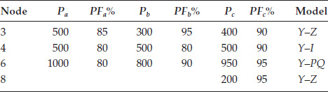
Delta-connected loads:

images

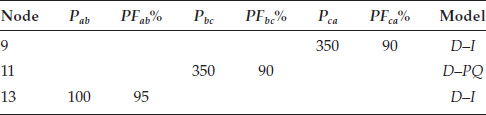
Create this system in Windmil.
Run voltage drop with the regulator set to “none.” Do this in the Voltage Drop Analysis Manager.
Compute the R and X and voltage level for the voltage regulator.
1. Hand calculation
2. Windmil “Regulation Set”
3. Compare settings
Run voltage drop with the regulators set to “step”
1. What are the final tap positions?
2. Are these appropriate?
Add shunt capacitors so that the source power factor is no lower than 95% lag. Specify capacitors in multiples of 100 kvar.
Run voltage with the final capacitors.
1. What is the power factor by phase at the source?
2. What are the final tap positions for the regulators?

References

1. Trevino, C., Cases of difficult convergence in load-flow problems, IEEE Paper n.71–62-PWR, Presented at the IEEE Summer Power Meeting, Los Angeles, 1970.

2. Kersting, W. H. and Mendive, D. L., An application of ladder network theory to the solution of three-phase radial load-flow problems, IEEE Conference Paper,Presented at the IEEE Winter Power Meeting, New York, 1976.

3. Radial Test Feeders, IEEE Distribution System Analysis Subcommittee, http://ewh.ieee.org/soc/pes/dsacom/testfeeders/index.html.

4. Kersting, W.H. and Phillips, W. H., Distribution system short-circuit analysis, 25^th Intersociety Energy Conversion Engineering Conference, Reno, NV, 1990.

5. Kersting, W.H., The simulation of loop flow in radial distribution analysis programs, IEEE Conference Paper,Presented at the IEEE Rural Electric Power Conference, 2014.

6. Kersting, W. H. and Carr, W., Grounded wye–delta transformer backfeed short-circuit currents, IEEE Conference Paper,Presented at the IEEE Rural Electric Power Conference, 2016.

..................Content has been hidden....................

You can't read the all page of ebook, please click here login for view all page.

Table of Contents for
10. Distribution Feeder Analysis