
Chapter Syllabus
Networking is a huge subject covering everything from a simple point-to-point serial connection to wide area networks spanning the globe. We can't possibly cover every technology in this one book. In HP-UX arenas, we traditionally focus on local to metropolitan networks. Beyond that, we talk to those guys with their heads stuck down a cabling duct who tells us where to plug in our RJ-45 connector. Our data disappears into that elusive big fluffy-cloud that network engineers love to draw to represent wide area networks. This chapter is not going to go into every facet of network technologies, but simply introduces some of the key technologies used in inter-networking that we, as HP-UX administrators, might not get involved with much. Just because it's the domain of the guy with his head down a cabling duct doesn't mean we shouldn't at least have an appreciation of these technologies. We discuss two typical WAN solutions from a basic theoretical perspective: Frame Relay and ATM. We move the discussion on ATMinto a discussion on Storage Area Networks (SANs). Some would say that a SAN is technically not a network. I would have to disagree. When most people think of a SAN, they think of Fibre Channel. If that is the case, then you must think of Fibre Channel as just another network technology. Currently, the vast numbers of Fibre Channel installations are there to support the SCSI protocol, i.e., to communicate with disk and tape devices. Fibre Channel supports many upper-layer protocols, including IP. We look at how WAN solutions are currently interfacing with SAN solutions in the context of DWDM, and long-haul asynchronous data replication. We conclude with a brief discussion on two other emerging network architectures: Virtual LANs and Virtual Private Networks.
Most modern Wide Area Network (WAN) protocols including TCP/IP, X.25, and Frame Relay are based on packet-switching technologies. In contrast, normal telephone service is based on a circuit-switching technology, in which a dedicated line is allocated for transmission between two parties. Circuit switching is ideal when data must be transmitted quickly and must arrive in the same order in which it's sent. This is the case with most real-time data, such as live audio and video. Packet switching is more efficient and robust for data that can withstand some delays in transmission, such as email messages and Web pages. Each packet is transmitted individually and can even follow different routes to its destination. Once all the packets forming a message arrive at the destination, they are recompiled into the original message.
Frame Relay is a high-performance WAN protocol that operates at the physical and data link layers of the OSI seven-layer model. Frame Relay was originally designed for use across Integrated Services Digital Network (ISDN) interfaces. Today, it is used over a variety of other network interfaces as well. Frame Relay is an example of a packet-switched technology. Packet-switched networks enable end stations to dynamically share the network medium and the available bandwidth. Two techniques are used in packet-switching technology:
Variable-length packets
Statistical multiplexing
Variable-length packets are used for more efficient and flexible data transfers. These packets are switched between the various segments in the network until the destination is reached. Statistical multiplexing techniques control network access in a packet-switched network. The advantage of this technique is that it accommodates more flexibility and more efficient use of bandwidth. Most of today's popular LANs, such as Ethernet and Token Ring, are packet-switched networks. Frame Relay is often described as a streamlined version of X.25, offering fewer of the robust capabilities, such as windowing and retransmission of last data that are offered in X.25. This is because Frame Relay typically operates over WAN facilities that offer more reliable connection services and a higher degree of reliability than the facilities available during the late 1970s and early 1980s that served as the common platforms for X.25 WANs. Frame Relay is strictly a Layer 2 protocol suite, whereas X.25 provides services at Layer 3 (the network layer) as well. This enables Frame Relay to offer higher performance and greater transmission efficiency than X.25, and makes Frame Relay suitable for current WAN applications, such as LAN interconnection. Devices attached to a Frame Relay WAN fall into two general categories:
Data terminal equipment (DTE)
DTEs generally are considered to be terminating equipment for a specific network and typically are located on the premises of a customer. In fact, they may be owned by the customer. Examples of DTE devices are terminals, personal computers, routers, and bridges.
Data circuit-terminating equipment (DCE)
DCEs are carrier-owned inter-networking devices. The purpose of DCE equipment is to provide clocking and switching services in a network, which are the devices that actually transmit data through the WAN. In most cases, these are packet switches.
One of the most commonly used physical layer interface specifications is the recommended standard (RS)-232 specification. The link layer component defines the protocol that establishes the connection between the DTE device, such as a router, and the DCE device, such as a switch.
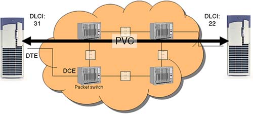
Frame Relay provides connection-oriented data link layer communication. This means that a defined communication exists between each pair of devices and that these connections are associated with a connection identifier. This service is implemented by using a Frame Relay virtual circuit, which is a logical connection created between two data terminal equipment (DTE) devices across a Frame Relay packet-switched network (PSN).
Virtual circuits provide a bidirectional communication path from one DTE device to another and are uniquely identified by a data-link connection identifier (DLCI). A number of virtual circuits can be multiplexed into a single physical circuit for transmission across the network. This capability often can reduce the equipment and network complexity required to connect multiple DTE devices. A virtual circuit can pass through any number of intermediate DCE devices (switches) located within the Frame Relay PSN.
Frame Relay virtual circuits fall into two categories:
Switched virtual circuits (SVCs)
Permanent virtual circuits (PVCs)
Switched virtual circuits (SVCs) are temporary connections used in situations requiring only sporadic data transfer between DTE devices across the Frame Relay network. A communication session across an SVC consists of the following four operational states:
Call setup: The virtual circuit between two Frame Relay DTE devices is established.
Data transfer: Data is transmitted between the DTE devices over the virtual circuit.
Idle: The connection between DTE devices is still active, but no data is transferred. If an SVC remains in an idle state for a defined period of time, the call can be terminated.
Call termination: The virtual circuit between DTE devices is terminated.
After the virtual circuit is terminated, the DTE devices must establish a new SVC if there is additional data to be exchanged. It is expected that SVCs will be established, maintained, and terminated using the same signaling protocols used in ISDN.
Few manufacturers of Frame Relay DCE equipment support switched virtual circuit connections. Therefore, their actual deployment is minimal in today's Frame Relay networks.
Previously not widely supported by Frame Relay equipment, SVCs are now the norm. Companies have found that SVCs save money in the end because the circuit is not open all the time.
Permanent virtual circuits (PVCs) are permanently established connections that are used for frequent and consistent data transfers between DTE devices across the Frame Relay network. Communication across PVCs does not require the call setup and termination states that are used with SVCs. PVCs always operate in one of two operational states:
Data transfer: Data is transmitted between the DTE devices over the virtual circuit.
Idle: The connection between DTE devices is active, but no data is transferred. Unlike SVCs, PVCs will not be terminated under any circumstances when in an idle state.
DTE devices can begin transferring data whenever they are ready because the circuit is permanently established (Figure 23-1).
Up to 976 DLCI (Permanent Virtual Circuits) per port provide the ability to establish a large number of user sessions. The frame size can be tuned up to 4096 bytes, enabling efficient data transfer. Support of IP access over Frame Relay (RFC 1490) enables IP applications to run over frame relay networks.
For each DLCI, the Committed Information Rate (CIR), Committed Burst Size (CBS), and Excess Burst Size (EBS) Traffic Management parameters can be configured, allowing tuning for optimum throughput. Frame Relay provides no explicit flow control per DLCI, but instead very simple congestion notification mechanisms, namely FECN and/or BECN (Forward and/or Backward Explicit Congestion Notification). Integration with HP-UX utilities such as SAM ensures easy installation and configuration. Monitoring and statistics are provided to help tuning and troubleshooting. Frame Relay allows communications between an HP 9000 system and other equipment (HP or non-HP) over Frame Relay (WAN) networks, using the TCP/IP services. The MTU size is configurable within the range 260 to 4000 bytes.
HP-UX J3529A Frame Relay software runs on HP 9000 server systems and workstations (EISA or PCI bus) running HP-UX 11i, as seen in Table 23-1.
Asynchronous Transfer Mode is a network technology based on transferring data in cells or packets of a fixed size. The cell used with ATM is relatively small compared to units used with older technologies. The small, constant cell size allows ATM equipment to transmit video, audio, and computer data over the same network, and assures that no single type of data hogs the line. ATM creates a fixed channel, or route, between two points whenever data transfer begins. This differs from TCP/IP, in which messages are divided into packets and each packet can take a different route from source to destination. This difference makes it easier to track and bill data usage across an ATM network, but it makes it less adaptable to sudden surges in network traffic. When purchasing ATM service, you generally have a choice of four types of service:
Constant Bit Rate (CBR) specifies a fixed bit rate so that data is sent in a steady stream. This is analogous to a leased line.
Variable Bit Rate (VBR) provides a specified throughput capacity, but data is not sent evenly. This is a popular choice for voice and videoconferencing data.
Available Bit Rate (ABR) provides a guaranteed minimum capacity, but allows data to be bursted at higher capacities when the network is free.
Unspecified Bit Rate (UBR) does not guarantee any throughput levels. This is used for applications, such as file transfer, that can tolerate delays.
An ATM cell is the smallest item an ATM network ever deals with. ATM cells may then pass into Multiplexed channels in a trunk (or backplane). TDM (Time Division Multiplexing) has been used in the past, but ATM recognizes that traffic is usually bursty in each of the multiplexed channels and so does not time slice. Instead, it adds a header to each cell in order and takes them on a first-come, first-serve basis. Bandwidth is allocated only to channels that have data to transmit, therefore, sharing the full bandwidth among the remainder. ATM is useful to implement where the traffic is packet orientated and so will often be used not only by packet-switch manufacturers but also in intelligent (multi-function) hubs as well. ATM is also the technology that B-ISDN is based on and will be used to provide many WAN services.
ATM at OSI Layer 2, like Frame Relay, uses 5 bytes (octets) for the header; add 48 bytes (384 bits) of payload data and you have a cell size of 53 bytes. ATM also has an upper level 2 layer known as the AAL (ATM Adaptation layer). It is used to determine the type of data, Constant or Variable length and Connectionless or Connection oriented. At present, there are five different classes.
Because this is a cell-switching technology, it also uses Virtual Connections, which are either Permanent (PVC) or Switched (SVC). A virtual path identifier (VPI) and virtual channel identifier (VCI) in the header identifies each cell.
Permanent Virtual Connections (PVC): A PVC is a connection set up by some external mechanism, typically network management, in which a set of switches between an ATM source and destination ATM system are programmed with the appropriate VPI/VCI values. As is discussed later, ATM signaling can facilitate the setup of PVCs, but by definition PVCs always require some manual configuration. As such, their use can often be cumbersome.
Switched Virtual Connections (SVC): An SVC is a connection that is set up automatically through a signaling protocol. SVCs do not require the manual interaction needed to set up PVCs and, as such, are likely to be much more widely used. All higher layer protocols operating over ATM primarily use SVCs.
Like Frame Relay, there are two different cell structures depending on whether it is a User Network Interface (UNI) cell or a Network Node Interface (NNI) cell. Both have a 5-byte (octet) header; the difference is what's in these 5 bytes. A UNI connects ATM end systems (hosts, router, and so on) to an ATM switch, while an NNI is a physical or logical link across which two ATM switches communicate.
The physical layer of ATM is divided into two sublayers. The TC or TCS (Transmission Convergence Sublayer) sits on top of the PMD (Physical Medium Dependant sublayer). TCS looks after cell delineation (how to identify the start and end of each cell) and cell rate decoupling (inserting empty cells during idle periods). Many of the TC standards also define some form of enveloping a number of cells so that it can check overall clocks and errors, and so on. At present, there are four main groups defined in the TCS:
SONET/SDH (normally at 155Mbits/sec): SONET (Synchronous Optical NETwork) is now an ANSI standard defining interface standards at the physical layer of the OSI seven-layer model. SDH (Synchronous Data Hierarchy) is a North American equivalent of SONET.
PDH (Plesiochronous Digital Hierarchy): The standard that controls the variance a data stream can take from its nominal speed. For a DS1/T1 link, this equates to 100 bits per second either side of 2Mbps. See http://www.dis.port.ac.uk/~earlyg/dins/l11/Lec11_98.html for a good talk on PDH.
Cell based (same coding as Fibre Channel):
A replacement for FDDI: This is the same coding and fibre, although obviously the FDDI card will still have to be replaced for an ATM card, and the actual physical connectors are different (FDDI uses a MIC, while ATM normally uses SC connectors in this situation).
PMD looks after the physical medium, line coding, and bit timing. The ATM Forum (http://www.atmforum.com) has tried to use existing standards wherever possible. There are numerous physical layer connections available for ATM, although HP-UX currently supports only a few. If you browse to http://www.atmforum.com/standards/approved.html and click “Physical Layer.” you will find all of the possibilities currently defined. HP's current offering include the solutions listed in Table 23-2.
Table 23-2. HP ATM Solutions
Adapter | Link Speed | Cable |
|---|---|---|
A5483A | 622Mbps | Multi-mode Fibre with SC connectors |
A5513A | 155 Mbps | Multi-mode Fibre with SC connectors |
A5515A | 155 Mbps | UTP Cat5 |
J2469A | 155 Mbps | Multi-mode Fibre with SC connectors Single-mode Fibre with SC connectors UTP Cat5 |
J2499A | 155Mbps | Multi-mode Fibre with SC connectors UTP Cat5 |
J3575A | 622Mbps | Multi-mode Fibre with SC connectors |
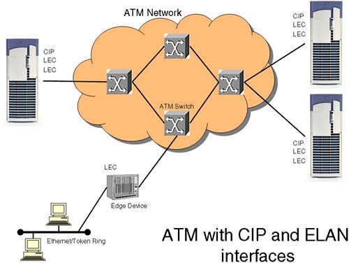
Where ATM fits into the OSI seven-layer model is a bit of a controversy. Most people would agree that it fits snuggly into Layer 2, but some would argue that it is quite happy as a Layer 3 product as well. This is true because the addressing scheme used by ATM exhibits all the characteristics of a Layer 3 protocol, including a hierarchical addressing scheme and a complex routing protocol. This leads to issues surrounding support of IP over ATM. If ATM has a complex routing protocol, how does IP interact with it? This is resolved by ATMARP software running on nodes that resolves ATM 40-bit hardware addresses to IP addresses. RFC 1577 covers the support of IP over ATM. Each interface card supports one Classical IP (CIP) address and up to 32 Emulate LAN (ELAN) interfaces configured as LAN Emulation Clients (LEC), each with a different subnet address. Nodes connected via an ATM switch that have LAN interfaces configured on the same subnet will form a Logical IP Subnet (LIS) with one node acting as the ATMARP Server, resolving ATM addresses to IP addresses, and the other acting as ATMARP Clients. ATMARP replaces the functionality of the ARP protocol. To communicate with other IP devices, the LIS will have to communicate via an ATM/IP edge device that can interface between an ATM network and a traditional Ethernet/Token Ring network.
ATM has many physical interfaces that it can utilize. The buzzwords in the industry are sometimes misleading, misunderstood, or used just to baffle us with science. In the end, they are a measure of the investment made by telecom companies in the quality of the infrastructure they support. We pay for available capacity. Most of the solutions these days utilize fibre optic cabling. Big numbers are used to try to impress us. As mentioned previously, only certain interface cards are supported by HP-UX. These equate to certain physical interface standards at Layer 2 of the OSI seven-layer model. While there are only a couple of interface standards supported for native ATM interfaces, these transmission speeds are not the only speeds available. It is not uncommon to have site-to-site ATM communications utilizing a “big fat pipe” with multiple edge devices giving access to existing 10/100/1000-BaseT networks. Ultimately, we need to consider what our overall solution is trying to accomplish. For example, if we are simply providing login capabilities for users in one site to another, we might not need as much bandwidth as if we are replicating data from one high performance disk array to another. Bandwidth is a fundamental part of a solution. If we know how much data we are likely to shift from site to site, we can start to focus on a particular solution. Table 23-3 shows links speed commonly used for serial communications.
These names are derived from international standards such as the Synchronous Data Hierarchy (SDH), which has a North American equivalent known as SONET (Synchronous Optical NETwork: now an ANSI standard defining interface standards at the physical layer of the OSI seven-layer model). It is for historical (or is it hysterical?) reasons that the standards are different on either side of the Atlantic.
Let's look at an example of where we need to backup 6TB of data overnight. Which solution would we go for? First, the answer is not entirely clear from a pure bandwidth measurement. We would need to establish the sustainable data rate that excludes any network headers, and so on, that will decrease the amount of pure data being transmitted over the link. Talk to your telecom supplier about this. Putting that aside, we need to transform our 6TB in 24 hours into a bandwidth figure we see above. It's a case of understanding the math in the end:
*OC = Optical Carrier *STM = Synchronous Transport Mode | ||
|---|---|---|
OC-12c/STM-4 | = | 622 Mb/second |
= | 77.75 MB/second | |
= | 279,900 MB/hour (≈ 273 GB/hour) | |
≈ | 6.4 TB/day | |
If this is the requirement, then we need to consider how we are going to achieve this. With a current native ATM solution for HP-UX, we can sustain 622 Mb/second. This solution is within our grasp (just). One of the questions we need to ask ourselves is this: Can our servers sustain 622 Mb/second for the length of an entire backup? For a backup solution, it is not uncommon to have our disk arrays (assuming that it is a disk array holding our data) communicating with the other device (another disk array possibly) on a remote site to perform our offsite backups. Such a solution would require intelligent disk arrays able to perform server-less backups. This solution is within the grasp of products such as DataProtector. This is where a program module is loaded on the disk array to communicate (usually over Fibre Channel) to another disk array without sending data via the server that initiated the backup. In this solution, we are using ATM, not as an IP-driven network but purely as an ATM backbone able to deliver packets of data, quickly and reliably. The edge device in this situation is not interfacing with an Ethernet/Token Ring network but with an ATM/Fibre channel bridge, converting FC frames to ATM frames and transmitting them on the ATM network. While some administrators would venture that this is not technically a network solution, I think we can now say that it is most definitely a network solution. ATM is more than capable at networking. The fact that it has been made to support IP is more through necessity than design. Currently, I would venture to say that ATM is used more in support of a Fibre Channel SAN than an IP network. I may be wrong, but in my experience that is where the investment is being made in ATM: long-haul, high bandwidth data replication. The cost of such a solution will depend on the telecom supplier you choose. When we think about it, the cost of lost data does not bear thinking about. I was privy to a solution in the UK where a financial institution was looking at laying 40 miles of fibre optic cable to support an ATM backbone. The cost? On average, the cost would have been £4 million to lay the cable alone. This sounds like lots of money, but in the total cost of the solution, £4M is not really that much. Think of the cost of losing IT functionality in a financial organization … it doesn't bear contemplating. £4M would be recouped in a matter of months, if not weeks. ATM is commonly used in a SAN environment to support SAN solutions over long distances. We take our discussions on other network technologies on to a discussion of basic SAN functionality and the role of WAN solutions in the context of long-haul data replication. This discussion also follows the train of thought regarding available bandwidth of a given ATM solution. While bandwidth is an important part of a solution, we must always consider propagation delays; how long does it take for a light signal to travel form London to New York? If you don't consider these types of questions, your overall solution may suffer.
We start our discussion with some brief definitions. In the world of HP-UX, sharing storage resources, i.e., disks and tapes over extended distance, will more than likely require us to use Fibre Channel. We implement a Storage Area Network (SAN) as our storage infrastructure. A SAN is a block-based transport architecture; for all intent and purposes, this means it's an interface that can support SCSI protocols. We use Fibre Channel for the following reasons:
It gives us the extended distances we require.
We can connect and, hence, share lots of devices
It provides high bandwidth and low latency.
It offers reliable transfers of data.
It is a completely separate physical and logical infrastructure from our IP-based LAN networks, hence, we are not contending with LAN traffic for access to existing bandwidth.
A simple explanation of the benefits of Fibre Channel is that it gives us the best of both worlds in terms of the familiarity of SCSI for interfacing with devices, as well as the familiarity of a LAN for extending connectivity over large distances. That's the way I think of Fibre Channel; a SCSI cable that can be miles long with hundreds (possibly millions) of devices connected to it. If that's how you want to think of Fibre Channel, I don't think you will be too far from the truth. I think understanding a SAN as simplistic and manageable is important. I have met many people who consider Fibre Channel and SANs as some form of voodoo cult with arcane rituals, chanting, and dancing around open fires. It isn't. Yes, it's relatively new. Yes, in the early days, getting suppliers to provide hardware that was compatible was nigh impossible (and that's still the case in some instances). Yes, new architecture does mean a new learning curve. But we said that about TCP/IP when it first came out. Look at us now; anyone who doesn't know the difference between a MAC address and an IP address probably needs to read another textbook before reading this one; we take IP addresses for granted these days. So let's reiterate it in as simplistic and manageable a form as we can. A SAN is a miles-long SCSI cable with hundreds of devices connected to it (devices can be disks, tapes, or other servers). Some of you may have come across something called a Network Attached Storage (NAS) device. A NAS device has two major distinctions over a SAN device. A major distinction is that an NAS device offers a file-based transport architecture. Some people I have spoken to said that an NAS-head (a common name for an NAS device that does the front-end processing of requests) is the natural evolution of a fileserver. NAS devices commonly support CIFS and/or NFS as their underlying filesystem to provide access to files over an existing IP network. The fact that a NAS-device offers a file-based transport architecture sees NAS device more commonly used in a Windows-type infrastructure. That's not to say we can't have NAS devices in a HP-UX infrastructure and vice versa; you could even have an NAS-head that is connected to a collection of disk devices using a backend SAN as their transport infrastructure. We are also seeing SAN protocols being supported over existing IP networks. I suppose the desire to utilize existing IP networks is a cost factor. However, we have to contend with the problem of congestion: Having block-based transport, i.e., SCSI requests, contending with our existing LAN traffic, all over the same infrastructure, must be seen as some form of compromise unless your IP network is offering very high bandwidth, low latency, and possibly even Quality of Service guarantees. For the near future, it seems that HP-UX lives in the world of SANs; it just seems that is the way it has panned out.
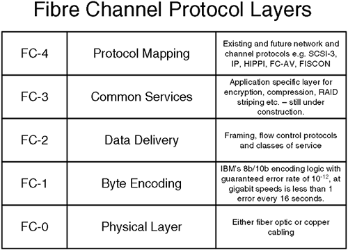
Fibre Channel is controlled by one of those committees (the NCIS/ANSI T11X3 committee to be precise) that produce those most interesting of documents: standards. In our world of networks, we know about standards and committees; in fact, if we think of the most prevalent model of networking, I would think you would agree it's the OSI seven-layer model. Fibre Channel as a set of standardized protocols is a layered architecture whose design is to transport data across a network. It consists of five layers FC-0 through to FC-4. Figure 23-3 gives you an idea of what each layer achieves.
Is this important? In the world of HP-UX, it's not terribly important that we understand every nuance of the standard. We need to get a handle on how this affects managing HP-UX. This includes managing devices files, and setting up, configuring, and managing clusters—two aspects of managing HP-UX that are immediately affected by implementing a Fibre Channel based SAN. Let's start from the ground up. I'm sure we all think Fibre Channel = fibre-optic, right? Probably, but not necessarily.
Fibre Channel standard FC-0 gives us two types of cabling to use: fibre-optic and copper cabling. Fibre optic cabling is the most commonly seen medium because it allows long cable runs. Fibre-optic cable comes in two forms:
Single-mode fibre: As the name might suggest, this type of fibre carries a light source of a single frequency. This means the cable core can be of a smaller diameter (9 μm = 9 micrometer). Using only a single, long-wave frequency means that we can carry a signal as much as 10km at gigabit speeds.
Multi-mode fibre: Here we are using multiple short-wave frequencies to transmit a signal. Using multiple frequencies requires a larger cable core. Multi-mode cable uses either a 62.5 μm or 50 μm core. You would think that having considerably more space in the cable core than single-mode fibre would enable us to carry a signal much further. Because of the short wavelength and the dispersion effects caused by using multiple frequencies, we can carry a signal only 175 meters with 62.5 μm cable and 500 meters with 50 μm cable.
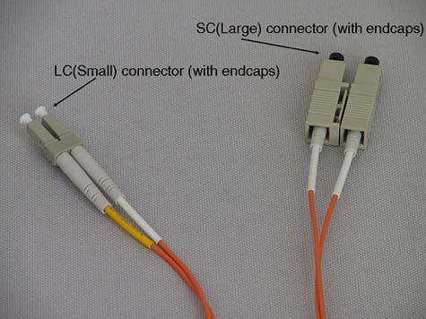
Both types of cable using 125 μm cladding that the light pulses reflect back into the core. Both types of cable also use a protective outer coating, usually in a distinctive orange color. You can usually determine which type of cable, because the manufacturer's name will be printed on the orange protective coating. The cable/connectors pictured in Figure 23-4 had printed on the orange protective coating “AMP Optical Fibre Cable 50/125” indicating 50 μm core with 125 μm cladding. Because it's such a thin cable, care should be taken not to trap it in suspended-floor tiles in computer rooms: The reflective cladding doesn't work very well with a hole in it.
Copper cabling is more commonly used to connect devices (read disks) within rack-mounting cabinets. Consequently, there are two types of copper cable:
Intracabinet copper: As the name suggest, all connections will be made within one cabinet and uses unequalized cabling limited to 13 meters.
Intercabinet copper: This is used to connect devices at longer distances, hence intercabinet. It uses active components (signal boosters) to push the signal to distances of up to 30 meters.
Currently, we see link speed of either 1 or 2 gigabits; however, 4 gigabits is on the near horizon. Our interface cards and other infrastructure components (that means switches) need to support the desired link speed. An interface card is commonly known as an HBA (host bus adapter). The most common connection between the HBA and the cable is via a GBIC (Gigabit Interface Converter). These are hot-swappable devices about the size of a box of matches. GBICs provide the signal to the physical medium with the HBA performing the serializing/de-serializing (serdes) of the signal.
Copper GBICs come in active (up to 30m) and passive (up to 13m) versions using either DB-9 or HSSDC (High Speed Serial Direct Connect) connectors.
Optical GBICs come in long wave (up to 10km) and short wave (up to 500m) versions. The power to drive an optical signal to these distances at 2GB/second appears to be a trial for some GBIC manufacturers, and it appears that GBICs running at these speeds seem to fail more than GBICs running at slower speeds. To go beyond 10km, some manufacturers offer Extended Long Wave GBICS that can push a light signal anything from 10km to 40, or even 80km in one hop. As always, developments in this field are fast and furious, with some suppliers claiming single-hop distances in excess of 100km that would normally require the use of Dense Wave Division Multiplexing (DWDM) devices. There are two types of connector for optical GBICs: SC (Standard) connectors or LC (Lucent) connectors. LC connectors are sometimes called SFF (Small Form Factor) connectors. It seems that SC/LC is a common name, and for some perverse, reason it is easier to remember which type of connect is which:
SC = LARGE connector
LC = SMALL connector
Figure 23-4 should help to remind you:
I suppose we will all have to get used to the fact that just about everyone else in the Fibre Channel word calls an interface card a Host Bus Adapter (HBA). I keep referring to them as interface cards, but in mixed company (when you have to speak to non-HP-UX folks), HBA seems to be the most common term. Every HBA has associated with it at least one address known as a WWN. If we take the analogy of a LAN card, every LAN card has (should have) a unique MAC address within a network. In a similar way, every HBA should have a unique identifier within the SAN. Manufacturers obtain a range of identifiers from the IEEE to uniquely identify HBAs from that manufacturer. The identifier comes in two parts: a 64-bit Node Name and possibly a 64-bit Port Name. Because these identifiers are globally unique, they are known as World Wide Names (WWN). An HBA will commonly have both a Node WWN and a Port WWN. “Why does it need both?” you ask. The answer is simple. Take a four-port Fibre Channel card. Each individual Port on the card needs to have a unique Port WWN, while the entire card might have a single Node WWN. Here comes the confusing part:
A node in a SAN is any communicating device, so a node could be a server or a disk.
A node in a SAN is identified as an N_Port device.
A node can have many individual connections associated with it; a server can have multiple HBAs, and each HBA may be a four-port Fibre Channel card.
Every individual connection from a node is associated with an individual N_Port identifier.
Every individual N_Port has to have a unique WWN associated with it.
Got it so far? Okay, so which WWN is used to identify an N_Port device, the Node WWN or the Port WWN? The answer is that an N_Port is associated with the Port WWN. Remember, the Node WWN may not be unique in the case of a four-port Fibre Channel card, but the Port WWN must be unique. Although the name used, i.e., an N_Port is the Port WWN, may be a little confusing at first, it does make some kind of sense. Someone once tried to liken a Node WWN to a server's hostname and the individual MAC addresses for individual LAN cards as Port WWNs. I suppose that's one way of looking at it. I think the fact that both the Node and Port WWN are of the same 64-bit format also makes it slightly confusing. Just remember that we use the Port WWN in our dealings with SANs and devices. In HP-UX, we can use a command such as fcmsutil to view the Node and Port WWN for our interface cards. First, we need to work out the device files for the individual ports. We do this with ioscan:
root@hp1[] ioscan -fnkC fc
Class     I  H/W Path  Driver S/W State   H/W Type     Description
=================================================================
fc        1  0/2/0/0   td   CLAIMED     INTERFACE    HP Tachyon TL/TS Fibre Channel Mass Storage Adapter
                      /dev/td1
fc        0  0/4/0/0   td   CLAIMED     INTERFACE    HP Tachyon XL2 Fibre Channel Mass Storage Adapter
                      /dev/td0
root@hp1[]
Here we can see that we have to separate Fibre Channel cards, both with a single Fibre Channel port. The device files being /dev/td0 and /dev/td1. We can now use fcmsutil to view the Node and more importantly the Port WWN:
root@hp1[] fcmsutil /dev/td0

                           Vendor ID is = 0x00103c
                           Device ID is = 0x001029
                XL2 Chip Revision No is = 2.3
            PCI Sub-system Vendor ID is = 0x00103c
                   PCI Sub-system ID is = 0x00128c
                               Topology = PTTOPT_FABRIC
                             Link Speed = 2Gb
                     Local N_Port_id is = 0x010200
            N_Port Node World Wide Name = 0x50060b000022564b
            N_Port Port World Wide Name = 0x50060b000022564a
                           Driver state = ONLINE
                       Hardware Path is = 0/4/0/0
                 Number of Assisted IOs = 3967
        Number of Active Login Sessions = 0
                   Dino Present on Card = NO
                     Maximum Frame Size = 960
                         Driver Version = @(#) PATCH_11.11: libtd.a : Jun 28 2002, 11:08:35, PHSS_26799

root@hp1[]
root@hp1[] fcmsutil /dev/td1

                           Vendor ID is = 0x00103c
                           Device ID is = 0x001028
                 TL Chip Revision No is = 2.3
            PCI Sub-system Vendor ID is = 0x00103c
                   PCI Sub-system ID is = 0x000006
                               Topology = PTTOPT_FABRIC
                     Local N_Port_id is = 0x010300
            N_Port Node World Wide Name = 0x50060b000006be4f
            N_Port Port World Wide Name = 0x50060b000006be4e
                           Driver state = ONLINE
                       Hardware Path is = 0/2/0/0
                 Number of Assisted IOs = 2557
        Number of Active Login Sessions = 0
                   Dino Present on Card = NO
                     Maximum Frame Size = 960
                         Driver Version = @(#) PATCH_11.11: libtd.a : Jun 28 2002, 11:08:35, PHSS_26799

root@hp1[]
In a simple point-to-point topology, one N_Port would connect directly to another N_Port, i.e., a server would be directly connected to a disk/disk array – nice and simple. When we consider other topologies, we realize that the Port WWN is not sufficient to identify nodes in a large complicated SAN. In particular, when we look at Switched Fabric topology, we realize that to route frames through the SAN the Fabric needs the intelligence to identify the Shortest Path from one node to another. It can't do this by just using the Port WWN. The Fabric must use some other identification scheme to identify N_Ports that will allow it to use some form of routing protocol. The routing protocol it uses is known as FSPF (Fibre Shortest Path First) and is a subset of OSPF packet routing in an IP network. Before getting into details about Switched Fabric, let's discuss other topology options.
Fibre Channel supports three topologies: Point-to-Point, Switched Fabric, and Arbitrated Loop. Of the three, Switched Fabric is the most prevalent nowadays. Point-to-Point is simply a server connected to a storage device; this is taking our concept of a mile-long SCSI cable just a little too far! Arbitrated Loop (FC-AL) was common a few years ago while the Switched Fabric products where becoming available. Nowadays, FC-AL is less common. It has lost favor because of its expansion and distance limitations as well as being a shared bandwidth architecture.
Although the FC-AL uses a 24-bit address, not all the bits are actually used (the top 16 bits are set to zero). We would assume that the remaining 8 bits could be used for FC-AL addressing giving us 28 = 256 addresses. Not so. The requirements of the 8b/10b encoding scheme in FC-1 mean that we only have 127 addresses (known as an AL_PA: Arbitrated Loop Physical Address) available. Each device has a unique address assigned during a Loop Initialization Protocol (LIP) exchange. Some devices have the ability to have their AL_PA set by some hardware or software switches. An AL_PA also reflects the priority of the device: The lower the number, the higher the priority. It would seem that 127 devices is adequate for most small(ish) installations. It is unlikely that you would ever use more than 10-20 devices in a FC-AL environment. One main reason is distance.
FC-AL is a closed-loop topology. Access to the loop is via an arbitration protocol. As the number of device increases, the chance of gaining access to the loop falls. When you introduce distance into the equation, FC-AL's arbitration can be seen to consume large proportions of the available bandwidth. The Fibre Channel FC-0 standard allows us 10km run of single-mode fibre-optic cable utilizing long-wave transceivers. Light propagates through fibre-optic at approximately 5 nanoseconds/meter. With a 10km run, that equates to a 50-microsecond propagation delay in one direction, or 100-microsecond roundtrip delay. The distance between individual devices calculates the total circumference of the loop. Taking a few 10km runs would consume vast tracks of the available, limited bandwidth; the 100-microsecond delay above equates to 1MB/second in bandwidth terms. It has been shown that beyond 1km FC-AL performance drops of considerably (anything up to 50 percent performance degradation).
Another problem with FC-AL is that it is a shared transport. That is to say, all devices share the available bandwidth. For example, when we get to 50 devices on a 1Gb/second (~100MB/second) Fibre, each device will have on average only 2 MB/second of bandwidth; that's not much. Take a small FC-AL SAN where we have one server connected to a RAID-box of six disks. The RAID-box operates RAID 5 across all disks, and each SCSI disk is operating at approximately 15MB/second. We can see that if the server is providing a service such as streaming video with larger sequential data transfers, all six disks and the server itself are already consuming the entire bandwidth available to FC-AL. Adding more disks would only exacerbate the bandwidth problem, although it would give us more storage.
Another problem with FC-AL has to do with what happens during a LIP. When a new node joins the loop, it will send out a number of LIPs to announce its arrival and to determine its upstream and downstream neighbors. This seems okay. However, if a node's host bus adapter (HBA; a Fibre Channel interface card to you and me) is faulty and loses contact with the loop, it can get into a situation where it starts a LIP storm. During a LIP, no useful data transmissions can occur. Take a situation with a tape backup. Even with a minor LIP storm, a backup will commonly fail because the device is effectively offline while the LIPs are being processed. Remember that RAID-box we saw previously? If we had to change a faulty disk, this would cause a minor LIP storm, and that's not good.
FC-AL commonly utilizes a Loop Hub to interconnect devices. Alternately, you could wire the transmit lead of one node to the receive port of another device, but that's unlikely because adding device into the loop is troublesome; remember trying to add nodes into a LAN where we used coaxial cable without losing network connectivity for everyone? What a nightmare! Like a LAN hub, a Loop Hub provides a convenient interface to connect devices together. Also like a LAN hub, a Loop Hub has little intelligence other than routing requests between individual ports. Devices connected through a Loop Hub are said to be in a private loop, i.e., they have no notion of anything outside their own little world. The reason for maintaining FC-AL devices is that they may be older devices where the HBA cannot operate in a Switched Fabric configuration. It may be desirable to make these devices available to the rest of the Switched Fabric devices. To be able to do this, the HBA in the device must be able to interact with other Fabric-aware devices. While being able to understand full 24-bit Switch Fabric addresses and perform a Fabric Login (FLOGI) to identify itself within the Fabric, it also must be able to communicate with local loop devices. Not all FC-AL HBAs can exist as public loop devices. If they do support operating as public loop devices, connecting the previously private loop to a Fabric Switch can allow us to migrate the private loop to a public loop. We would plug one of the ports from our Loop Hub into the switch. The switch port will perform a LIP, realize it is participating in a FC-AL, and assume the highest priority AL_PA=0x00; the switch port will operate in a mode known as an FL_port. It is the fact that a private loop is connected to an FL_Port that transforms it into a public loop. In making the private loop a public loop, other devices connected to the Fabric can now communicate with these devices. We also get the benefit of using a Fabric Switch that allows us to maximize the throughput a switch gives us; each port on the switch can support full duplex, 1 or 2Gb/second bandwidth to every other port simultaneously. If the switch port were configured to simply remain a loop port (known as an NL_port) because the devices on the private loop could not operate in a public loop, these devices would not be accessible via the rest of the Fabric. This is not good for older, legacy devices. The Fibre Channel standards do not care for this situation. It is not a requirement of any Fibre Channel standard to provide Fabric support to non-fabric devices. As you can imagine, customers would find it rather annoying for some standards-body to come along and decree that all your old legacy devices were now defunct; in order for you to go full-fabric, you would have to upgrade all the HBAs in all your old non-fabric devices. As you can imagine, although it is not a requirement of any standard, many switch vendors support this notion on non-fabric devices being accessible via a fabric. Effectively, the NL_port on the switch will take all requests for the private loop devices and translate the destination ID into a valid address within the Fabric. This mechanism of providing private non-Fabric functionality via multiple switch ports has various names depending on the switch vendor. Supporting private loop on a switch is sometimes known as phantom mode. Other names include stealth mode, emulated private loop (EPL), translative mode, and Quickloop. Some switches can support this, but others can't. FC-AL devices communicating in this way are completely unaware of the existence of a Fabric and are therefore still operate as if they were private loop devices. This gets around the problem of non-fabric devices suddenly becoming defunct overnight because we have decided to roll out a Switched Fabric. It allows customers to connect what were separate, standalone private loops into one large virtual private loop. It also allows customers to use older legacy devices within their Fabric until such times as the HBA for that device can be upgraded to be Fabric aware. With all these different topology options, it becomes a challenge for us to identify which ports on a switch are supporting FC-AL, which ones are running in Phantom Mode, and which are supporting Switch Fabric. That will come later. Let's talk a little about Switched Fabric.
I would have to say that switched fabric is the topology of choice for the vast majority of SAN installations. It alleviates the problems of expansion, distance, and bandwidth seen with FC-AL. A Fabric is a collection of interconnected fabric switches. “Is a SAN a fabric?” you ask. Yes, a SAN can be seen as a Fabric. Remember, a SAN could alternately be a collection of cascading hubs supporting FC-AL, so the topology of Switched Fabric is a topology design decision when constructing a SAN. Because Switched Fabric is the current topology of choice, most people interchange their use of SAN and Fabric and never mind or even understand the difference. Now you know.
An individual switch is a non-blocking internal switching matrix that allows concurrent access from one port to any other port. It has anything from 8 to 256 individual ports. Smaller switches are sometimes called edge switches, while large switches are sometimes called core or director class switches due to their high configuration capabilities, extension configuration options, and extremely low latencies (as low at 0.5 μseconds), placing them at the core of a large extended Fabric. There is no formal distinction between a director class and an edge switch; it is more of an arbitrary distinction based on its configuration possibilities. Each port on a switch can operate at full speed and full duplex operation, which means that unlike a Loop Hub that has to share available bandwidth among all connected nodes, as we add more nodes to a switch, performance does not degrade for individual nodes. If you are a marketing-type person, you could even argue that performance increases in direct proportion to the number of nodes attached. This sounds rather suspect, doesn't it? But you can sort of see their point. The aggregate bandwidth of FC-AL does not change; it's a shared bandwidth topology. The aggregate bandwidth of a Switch Fabric will always increase, i.e., eight nodes all communicating a 100MB/second is an aggregate bandwidth of 800MB/second. Add another eight nodes, and your aggregate bandwidth is now 1600MB/second. I told you that you would have to see this through the eyes of a marketer; I suppose I have to concede it is actually a fact. Because each port is operating in concurrent mode with every other node simultaneously, we could almost say the individual communications between nodes are operating like a point-to-point connection. This is not an unreasonable comparison to make; in fact, some devices will designate a Switch Fabric connection as being of the form PP-Fabric, PTTOPT_Fabric, or something similar. The important point is that our interface is fabric aware and able to participate in a Switched Fabric topology. To do this, an HBA must perform a FLOGI or Fabric LOGIn.
When we interconnect switches, we start getting into more complicated territory. First, how does the Fabric know the Shortest Path (remember FSPF; the subset of the OSPF routing protocol) to an individual N_Port? When we connect a node to a switch, it goes through an initialization sequence (a bit more of that later). This process, known as FLOGI, is when the node identifies itself to a switch port by sending it a FLOGI frame containing its node name, Port WWN, and what services it can offer (services being things like which protocols a node supports, e.g., SCSI-3, IPv4, IPv6, and so on). At this time, the switch will assign a 24-bit N_Port ID to each node attaching to a port. This 24-bit address space is the same address space used by FC-AL, but unlike FC-AL, which was restricted to 8 bits, Switched Fabric uses the full 24 bits. Some of the addresses are reserved, so from the theoretical 224 = 16 million addresses, we can use only 15.5 million. If you are going to have more than 15.5 million nodes connected to your SAN, then you have a problem. As yet, no one has reached this limitation (hardly a surprise!). So we have another address to contend with. Well, I'm afraid that it's the N_Port ID. If we recall the output from the fcmsutil we saw earlier, we can spot the N_Port ID:
root@hp1[] fcmsutil /dev/td1

                           Vendor ID is = 0x00103c
                           Device ID is = 0x001028
                 TL Chip Revision No is = 2.3
            PCI Sub-system Vendor ID is = 0x00103c
                   PCI Sub-system ID is = 0x000006
                               Topology = PTTOPT_FABRIC
                     Local N_Port_id is = 0x010300
            N_Port Node World Wide Name = 0x50060b000006be4f
            N_Port Port World Wide Name = 0x50060b000006be4e
                           Driver state = ONLINE
                       Hardware Path is = 0/2/0/0
                 Number of Assisted IOs = 2557
        Number of Active Login Sessions = 0
                   Dino Present on Card = NO
                     Maximum Frame Size = 960
                         Driver Version = @(#) PATCH_11.11: libtd.a : Jun 28 2002, 11:08:35, PHSS_26799

root@hp1[]
It's not as bad as it sounds. We can't change the WWN, and the HBA/port sends the FLOGI frame all by itself. All we need to do is connect them together. The intelligence in the switch assigns an N_Port ID itself. The switch stores the Port WWN to N_Port ID mapping so it knows where you are. This database and the associated service that looks after it are known as the Simple Name Service (SNS). Every switch runs the SNS and maintains its own database of SNS objects. The intelligence in the N_Port ID is that it encodes which switch you are connected to within a Fabric. Not only does it tell you which switch you are connected to, but also which physical port you are connected to. The N-Port ID is a 24-bit address broken down into three 8-bit components of the following form
23← bits →16 | 15 ← bits →8 | 7 ← bits →0 |
Domain | Area | Port |
At first this might look a little daunting, because there are terms here we haven't met before. Actually, when we put these terms into something a little more understandable, it becomes clear:
Domain—. switch number. This means that a Fabric is limited to 28 = 256 interconnected switches. In fact, it is limited to 239 interconnected switches because 16 of the addresses are reserved. In reality, a Fabric never gets anywhere near the 239 maximum, although someday someone with lots of money and lots of cable might give it a try.
Area—. port number on the switch.
Port—. zero in a Switched Fabric; in FC-AL, this is the AL_PA.
When we look at the output from fcmsutil, we can see the N-Port ID:
Local N_Port_id is = 0x010300
This now makes sense because we can break this down as follows:
Domain—. switch number = 0x01 = Switch number 1.
Area—. port number on the switch = 0x03 – this HBA is connected to port3 on Switch 1.
Port—. = 0x00 = zero in a Switched Fabric; in FC-AL, this is the AL_PA.
We can extract the N_Port ID for this HBA by using the command fcmsutil. We could also see this by logging on to the switch and use the command nssshow.
When switches are connected together they pass information between each other. Included in this transfer of information is the SNS database maintained on each switch. So, when a server wants to communicate with a disk somewhere within the Fabric, it can query the SNS database on the switch it is connected to and see all devices in the entire Fabric that support the SCSI-3 protocol. When two nodes want to communicate over the fabric, the switches in the Fabric know where they are located because all the switches in the Fabric can query any SNS object connected to the Fabric and resolve its Port WWN to N_Port ID mapping.
So far, so good. Plug in a Fibre Channel card to a Fabric Switch and the switch gives its own identifier in order to route packets around the SAN. Easy! In the world of HP-UX, this N_Port ID is actually identifiable in the output from a fcmsutil command, so knowing how an N-Port ID is constructed helps us identify which paths our IO requests are taking through the SAN. In this way, we can evaluate whether we have any SPOFs in our SAN design by identifying individual paths to individual devices (disks). As well as using multiple HBAs, we should also use multiple switches with each HBA connecting into a separate switch. Individual switches can be connected together as well to provide additional paths and additional redundancy. In Figure 23-5, you can see a simple Switched Fabric SAN. In this example, not all connections (the ones to the disk arrays) have full redundancy. This is a less-than-optimal solution. The customer knows and accepts this and is willing to live with it.
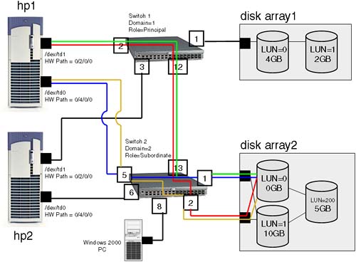
I am only concerned with the connections to LUN0—on disk array 2. Before we go any further, LUN0 is 0GB in size; it is not a typing mistake. If you want a full discussion on hardware paths and how device files are worked out in a SAN, have a look at Chapter 4: Advanced Peripherals Configuration. Let's return to the discussion at hand. The SNS on each switch will contain a mapping of all devices connected, so when a server wants to communicate with a particular disk, it will query the SNS and be returned the associated N_Port ID of the disk or disk arrays we want to communicate with. As far as HP-UX is concerned, an N_Port ID relates directly to an HP-UX hardware path of the device we are talking to—in this case, the disk arrays. Some people find this confusing and expect that the port number of the switch they are attached to and even the switch number they are attached to will somehow be included in the hardware patch seen by HP-UX. Any Inter Switch Links have nothing to do with an HP-UX hardware path for a disk or even a SCSI interface. Another way to look at this is if we go way back to our simplistic view of a SAN, it was a mile-long SCSI cable with hundreds of devices connected to it. If we think about it carefully, the end of our mile-long SCSI cable is going to be the last port we are connected to before we see a disk drive. In this example, our mile-long SCSI cable ends at either port 1 or port 2 on Switch2. We don't care how we got there; we just care that this is the end of our mile-long SCSI cable. Let's take a look at the hardware paths for the two connections from the server hp1 to LUN0 on disk array 2 (lost of the output from ioscan has been deleted to make this demonstration easier to follow):
root@hp1[] ioscan -fnC disk
Class     I  H/W Path      Driver   S/W State   H/W Type     Description
========================================================================
disk      9  0/2/0/0.2.1.0.0.0.0   sdisk    CLAIMED DEVICE    HP A6189A
disk     16  0/2/0/0.2.2.0.0.0.0   sdisk    CLAIMED DEVICE    HP A6189A
disk     13  0/4/0/0.2.1.0.0.0.0   sdisk    CLAIMED DEVICE    HP A6189A
disk      2  0/4/0/0.2.2.0.0.0.0   sdisk    CLAIMED DEVICE    HP A6189A
For the purposes of this discussion, the format of the hardware path can be broken down into three major components:
<HBA hardware path><N_Port ID><SCSI address>
Let's take each part in turn:
<HBA hardware path>: In this case, we have two HBAs on serverhp1, so the hardware path is going to be either0/2/0/0or0/4/0/0.<N_Port ID>: This is the N_Port ID of the device we are talking to, i.e., the interface for the disk arrays in this case, not the N_Port ID of our HBA. For me, this was something of a breakthrough. Each device is registered on the switch via its WWN to N_Port ID mapping, so the disk array connected to ports 2 and 3 on Switch2 have performed a FLOGI and the switch has associated their Port WWN with an N_Port ID. It is the disk arrays we are communicating with and, hence, it is the N_Port ID of the interfaces on the disk arrays we are concerned with in our HP-UX hardware path.This now starts to make sense. Back in Figure 23-3, we can see that the N_Port ID for all connections to
LUN0are via2.1.0or2.2.0, which translates to:Domain (switch number) = 2
Area (port on the switch) = 1 or 2
Port = 0
<SCSI address>: HP-UX hardware paths follow the SCSI-II standard for addressing, so we use the idea of a Virtual SCSI Bus (VSB), target, and SCSI logical unit number (LUN). The LUN number we see in Figure 23-3 is the LUN number assigned by the disk array. This is a common concept for disk arrays. HP-UX has to translate the LUN address assigned by the disk array into a SCSI address. If we look at the components of a SCSI address, we can start to work out how to convert a LUN number into a SCSI address:Virtual SCSI Bus: 4-bit address means valid values = 0 through 15.
Target: 4-bit address means valid values = 0 through 15.
LUN: 3-bit address mean valid values = 0 through 7.
There's a simple(ish) formula for calculating the three components of the SCSI address. Here's the formula:
Ensure that the LUN number is represented in decimal; an HP XP disk array uses hexadecimal LUN numbers, while an HP VA disk array uses decimal LUN numbers.
Virtual SCSI Bus starts at address 0.
If LUN number is < 12810, go to step 7 below.
Subtract 12810 from the LUN number.
Increment Virtual SCSI Bus by 110.
If LUN number is still greater than 12810, go back to step 4 above.
Divide the LUN number by 8. This gives us the SCSI target address.
The remainder gives us the SCSI LUN.
For our example, it is relatively straightforward:
LUN(on disk array) = 010
Is LUN number < 12810 ? If yes, then Virtual SCSI bus = 0
Divide 0 by 8 … SCSI target = 0
Remainder = 0 … SCSI LUN = 0
SCSI address =
0.0.0For an explanation of all the examples in Figure 23-3, including a discussion on the associated device files, go to Chapter 4: Advanced Peripherals Configuration.
I hope this is starting to make sense. It took me some time to grasp this, but eventually what made the breakthrough was that the concept of the mile-long SCSI cable ending at the last port on the last switch in the SAN gave me the N_Port ID of the device I want to communicate with. The rest of the hardware path was the SCSI components that I could calculate using the formula we saw above. If you have a JBOD (Just a Bunch of Disks) connected to your SAN, the SCSI addressing will be the simple SCSI addresses you set for each device within the JBOD.
I was going to finish my discussions on SANs in relation to HP-UX at this point. I decided to go a little further because in an extended cluster environment, we commonly have disks attached via Fibre Channel that are at some distant location. I thought it prudent to discuss some of the technologies you will see to provide an extended SAN.
We start this discussion by looking at the different port types we see in a SAN. This is useful if you ever have trouble communicating with a particular device. If it hasn't performed a FLOGI, it will not be participating in our Switched Fabric and this is a big indication as to why you can't communicate with it. One reason for this is that it may be a Windows-based machine that could be in its own private loop. In fact, this is a common problem for Windows-based machines, because we commonly need to tell the HBA to operate in Switched Fabric mode either via a software setting or by editing the Windows Registry. It is this reliance on software or device driver settings that can make the plug-and-play scenario not work as easily as we first thought. The vast majority of my dealings with HP-UX have been that the device driver you load will determine the topology used by the HBA. Most of the time, we simply need to plug our HBAs into a switch and understand the hardware path we see in ioscan. When this doesn't work, it can be useful to be able to decipher which HBAs are participating in our Switch Fabric and which ones aren't. We can do this by logging in to the switch and seeing which HBAs have registered and what topology they are operating under. Part of the registration/initialization process between the switch and the HBA will determine which topology the HBA is supporting. First, here's an idea of what happens when we connect something into a port on a switch:
Ports on a switch are known as Universal ports, which means that they can be connected to an Arbitrated Loop, a Switched Fabric, or another switch.
When two ports are connected, the Universal port on the switch will:
Perform a LIP. Essentially, this asks the other port (an HAB possibly) “Are you in an Arbitrated Loop?” If not, proceed to the next stage.
Perform a Link Initialization. Essentially, this asks the other port “Are you Switched Fabric?” If not, proceed to the next stage.
Send Link Service frames, which essentially means “You must be another switch, so let's start swapping SNS and other information.”
All this leads to the fact that we have different port types that will allow us to identify which topologies are in force for certain ports on our switch or hub:
N_Port: A node (server or device) port in a point-to-point or more likely a Switched Fabric.
NL_Port: A node (server or device) port operating in a FC-AL.
F_port: A switch port operating in a Switch Fabric.
FL_port: A switch port operating in FC-AL, connecting a public loop to the rest of the fabric.
E_Port: An Extension port. (A switch port connected to another switch port. Some switches allow multiple E_Ports to be aggregated together to provide higher bandwidth connections between switches. This aggregation of Inter Switch Links is known as ISL Trunking. To external traffic, the link is seen as one logical link.)
B_Port: A Bridge port. (This is not seen on a switch but on a device that will connect a switch to a Wide Area Network such as a bridge or router.)
QL_Port: Sometimes called Phantom, Stealth, or Translative Mode. (QL = Quickloop, which is a Brocade name so check with your switch vendor if they support this functionality. This is not a requirement of any Fibre Channel standard or protocol; it is used by switch vendors to allow customers to connect older non-fabric-aware private loop devices together via a switch. You see QL ports on switches. QL ports allow disparate private loops (loop-lets) to communicate with each other in a large virtual private loop.)
G_Port: A Generic port. (This is a port on a switch that can operate either as an F_Port or an E_port. You don't normally see G_Ports when looking at a switch.)
L_Port: A Loop port. (This is a port that can operate in an Arbitrated Loop. Node (NL_port) and fabric (FL_port) are examples of an L_Port. Sometimes, you will see a switch port specifying “L Port public” or “L port private” depending whether it's operating in a Public or Private Loop.)
Figure 23-6 is an example of a SAN that has implemented many of the port types listed above.
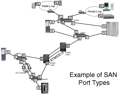
All of the devices in this SAN will be able to communicate with each other except the devices on the Private Loop. With the use of ATM to bridge between sites, this solution could span many miles; it could even span continents.
The first thing to mention when we connect switches together is compatibility. It would be helpful if all switches from every vendor could plug-and-play. Currently, this is a nirvana some way off in the distance. In my example in Figure 23-5, I simply plugged port 12 from Switch1 to port 13 of Switch2. The switches negotiated between themselves, and all was well. In a heterogeneous environment, we may have to jump through hoops to get this to work. Incompatibility between switch vendors is probably the main reason customers stick with one switch vendor. This is not to say that switches from the same vendor will automatically work when connected together. Here are some situations I have found myself in that caused same vendor switches not to work straight out of the box:
Incompatible Domain IDs: Every switch in a Fabric needs to have a unique Switch Domain. If not, the Fabric will become segmented with some switches and devices are not visible. The best solution is to power-up a switch and manually set the Domain ID on every switch. When a switch is introduced into a fabric and it does not have a unique Domain ID, part of the inter-switch negotiation allows for a Domain ID to be re-assigned. If this happens, it may have a detrimental effect on our configured hard zoning. The switch itself may not allow support for the reconfigure fabric link service. Most switches do, but I prefer to ensure that all switches have unique IDs before introducing them into a fabric.
Incompatible firmware versions: There was a classic problem with versions of firmware on HP/Brocade switches around the time of Fabric OS version 2.7. There was a switch parameter known as “Core Switch PID format.” The default prior to Fabric OS version 2.7 was OFF (0=zero). New switches (after Fabric OS version 2.7) had this parameter ON (1=zero). When connecting an old and a new switch together, the Fabric would be segmented. The solution was to change the parameter setting, and all was then okay. Not obvious. Even when we upgraded the firmware on the old switch, the parameter remained the same: contrary to the documentation for the firmware upgrade. So be careful.
Incompatible port configurations: Switches commonly allow for ports to be configured to allow/disallow certain port types to be configured. If we choose a port that has been configured E_Port_Disallow, then that port is not a good choice to connect two switches together. This needs to be checked on a switch-by-switch basis and a port-by-port basis. Most switches do not disallow port type by default, but it's worth remembering.
The easiest way to view port types is to log in to a switch. Most switches will have a 10/100 BaseT network connection that allows you to log in via the network and view/manage port settings. I would suggest you obtain permission from your friendly SAN administrator before doing this because you can make changes to a switch that will render it inoperable in an extended SAN like the example in Figure 23-6. Different switches have different command sets, so it is not easy to give generic examples. The switch I am about to log in to is an HP FC16 switch. It behaves much like a Brocade switch. Here are some example commands to look at port types and extended fabric configurations. To connect to a switch, you will need to know its IP address; otherwise, you will have to connect an RS-232 cable to the DB-9 connector on the front of the switch and onto a terminal/PC. To log in to the switch, you will need to know the administrator's username and password. I hope someone has changed them from being the default of admin/password! If you refer to Figure 23-5, I have two switches in my Fabric: Switch1 and Switch2. Here's how I viewed the port types as well as the extent of the Fabric:
Switch1:admin>
Switch1:admin> switchshow
switchName:     Switch1
switchType:     9.2
switchState:    Online
switchRole:     Principal
switchDomain:   1
switchId:       fffc01
switchWwn:      10:00:00:60:69:51:12:72
switchBeacon:   OFF
port  0: id N2 No_Light
port  1: id N1 Online       F-Port 50:06:0b:00:00:1a:0a:6c
port  2: id N2 Online       F-Port 50:06:0b:00:00:22:56:4a
port  3: id N2 Online       F-Port 50:06:0b:00:00:22:56:3c
port  4: id N2 No_Light
port  5: id N2 No_Light
port  6: id N2 No_Light
port  7: id N2 No_Light
port  8: id N2 No_Light
port  9: id N2 No_Light
port 10: id N2 No_Light
port 11: id N2 No_Light
port 12: id N2 Online       E-Port 10:00:00:60:69:51:4d:b0 "Switch2" (downstream)
port 13: id N2 No_Light
port 14: id N2 No_Light
port 15: id N2 No_Light
Switch1:admin>
Switch1:admin> fabricshow
Switch ID   Worldwide Name           Enet IP Addr    FC IP Addr      Name
------------------------------------------------------------------------
  1: fffc01 10:00:00:60:69:51:12:72  155.208.66.151  0.0.0.0  >"Switch1"
  2: fffc02 10:00:00:60:69:51:4d:b0  155.208.67.100  0.0.0.0   "Switch2"

The Fabric has 2 switches


Switch2:admin> switchshow
switchName:     Switch2
switchType:     9.2
switchState:    Online
switchMode:     Native
switchRole:     Subordinate
switchDomain:   2
switchId:       fffc02
switchWwn:      10:00:00:60:69:51:4d:b0
switchBeacon:   OFF
Zoning:         OFF
port  0: -- N2 No_Module
port  1: id N1 Online       F-Port 50:06:0b:00:00:19:6a:30
port  2: id N1 Online       F-Port 50:06:0b:00:00:19:65:0a
port  3: -- N2 No_Module
port  4: -- N2 No_Module
port  5: id N1 Online       F-Port 50:06:0b:00:00:06:be:4e
port  6: id N1 Online       F-Port 50:06:0b:00:00:06:c6:c6
port  7: -- N2 No_Module
port  8: id N1 Online       L-Port 1 public
port  9: -- N2 No_Module
port 10: -- N2 No_Module
port 11: -- N2 No_Module
port 12: -- N2 No_Module
port 13: id N2 Online       E-Port 10:00:00:60:69:51:12:72 "Switch1" (upstream)
port 14: -- N2 No_Module
port 15: id N2 No_Light
Switch2:admin>
Here we can see which Port WWNs are registered against each port. This is not the SNS database, which can be viewed with the nsshow command. To establish which host is connected to which port, we would tally the WWNs from switchshow with the output of fcmsutil run on each server. The 1 L-Port (port 8 on Switch2) is actually a Windows 2000 server.
It has to be stressed that the commands used here are specific for the type of switches I am using (HP FC16; similar to Brocade command set). Be sure to check with your vendor which commands are available (typing help after you're logged in to the switch is usually a good start).
One of the last things I want to mention in this (supposedly short) introduction to SANs is the concept of zoning. Refer to the SAN in Figure 23-6 and remember that all devices can communicate with all other devices (except devices in the private loop). This is sometimes a good thing when all servers need to be able to see all devices. However, this is seldom the case in reality. If we attach a Windows-based machine to our SAN and start creating LUNS on our disk arrays, the administrator on the Window-based machine will start to see a number of “Found New Hardware Wizard” screens popping up on his server. Most switches by default have no security enabled; we call this an Open SAN, i.e., everyone can communicate with everyone else's devices. There are basically two forms of security we can implement within a SAN:
LUN masking: This is the ability to limit access to particular LUNs, e.g., on a disk array, based on the WWN of the initiator. Few switches implement LUN masking. However, many disk array suppliers provide LUN masking software within their own disk arrays, e.g., Secure Manager/XP for HP XP disk arrays.
Zoning: This is the ability to segregate devices within the SAN. The segregation can be based on departmental, functional, regional, or operating system criteria; it is up to you. The problem we mentioned above regarding our Windows-based server grabbing new LUNs even though they were not destined for that machine would have been resolved by segregating Windows machines and their storage devices away from HP-UX machines and their storage devices. For example, we could have all HP-UX machines and their storage devices in an HP-UX zone with the Windows machines in a Windows zone. Zones can overlap, e.g., a TapeSilo zone for all our tape storage devices. HP-UX machines could belong to both an HP-UX and a TapeSilo zone to allow them to perform tape backups. The same could be true for the Windows zone.
A zone is a “collection of members within a SAN that have the need to communicate between each other.” When I use the word member, I do so for a reason. A member can be either:
A physical port on a switch
The WWN of a device within the SAN
This gives us two options in how we implement zoning. Each type of zoning has pros and cons:
Hard zoning: Based on the individual ports on individual switches
Pro: More secure, because it is based on the physical port number of a switch. This means spoofing a Fibre Channel header with bogus WWN information is virtually impossible. Another pro is that if a server changes its HBA (due to a hardware failure), the zoning is not affected.
Con: If someone moves the connection for a server between ports on a switch, that server may not be able to communicate with its disks/tapes anymore. Alternately, it may be able to communicate—and destroy—the devices for another group of machines.
Soft zoning: Based on WWN of devices within the SAN
Pro: The zoning stays with the device, so moving the connection for a server from one port to another has no effect on security.
Con: If a server changes its HBA (due to a hardware failure), the zoning configuration may have to be reworked.
Because zoning and security are becoming key features within a SAN, interoperability between vendors is becoming more and more common (although no guarantees can be given at this stage). Let's look at an example of the two switches I showed you earlier in Figure 23-5. Currently, there is no zoning in place, i.e., both servers can see all the LUNs configured on both disk arrays. If I wanted to implement zoning, I would have to sit down with my diagram and work out which members wanted to communicate with each other. I prefer hard zoning, primarily because of the security implications. In this example, my planning is relatively simple:
Server
hp1needs to communicate with all LUNs configured ondisk array2.Server
hp2needs to communicate with all LUNs configured ondisk array1.
With hard zoning, we need to work out which physical ports on particular switches need to communicate. Remember, the physical ports are our members in hard zoning. I can now give my zones names and assign ports to those zones. Ports are normally named <switch domain>,<port number>, e.g., 2,5 for switch domain = 2, port number = 5. The switch domain you can get from the output of the switchshow command. I hope we have established which servers are connected to which ports by tallying the WWN from the command fcmsutil with the output from switchshow. Here are the zones I have worked out:
Zone for server hp1 = HP1DATA
Ports (4 members):
1,2: server to switch1 port 1
2,5: server to switch2, port 5
2,1: disk array2 to switch 2, port 1
2,2: disk array2 to switch 2, port 2
Zone for server hp2 = HP2DATA
Ports (3 members):
1,3: server to switch 1, port 3
2,6: server to switch 2, port 6
1,1: disk array1 to switch 1, port 1
Most switches allow you to configure aliases for members. For example, hp1td0 could be an alias for member 2,5, in other words, the connection from server hp1 to the switch via Fibre Channel interface /dev/td0. This can make your configurations much easier to understand but is not obligatory. Another thing to watch is that some switch vendors may require you to include E_Ports into your zones. In this case, I would need to include member 1,12 and 2,13 into both zones. With my particular switches, this is not necessary. Once you have planned out your zoning, it is time to start configuring it. Here is my cookbook approach to setting up zoning (I have included the commands I used on my switches for demonstration purposes):
Establish which switch is the Principal Switch in your Fabric. The Principal Switch assigns blocks of addresses to other switches in the fabric to ensure that we do not have duplicate addresses within the Fabric. The selection of a Principal Switch is part of the inter-switch negotiation. Using the
switchshowcommand shows you theSwitchRole(see output above). In my two-switch Fabric, it so happens thatSwitch1is the Principal Switch. Using the Principal Switch to configure zoning ensures that all configuration changes are propagated to all Subordinate Switches.Set up any aliases you will use for nodes in the Fabric.
Switch1:admin> alicreate "hp1td0","2,5"
Switch1:admin> alicreate "hp1td1","1,2"
Switch1:admin> alicreate "hp1RA1CH1","1,1"
Note for my naming convention:
hp1RA1CH1hp1= server nameRA1= disc array1CH1= channel 1 (interface on disc array)Switch1:admin> alicreate "hp2td0","2,6" Switch1:admin> alicreate "hp2td1","1,3" Switch1:admin> alicreate "hp2RA2CH1","2,1" Switch1:admin> alicreate "hp2RA2CH2","2,2"
Establish individual zones.
Switch1:admin> zonecreate "hp1DATA","hp1td0; hp1td1; hp1RA1CH1"
Switch1:admin> zonecreate "hp2DATA","hp2td0; hp2td1; hp2RA2CH1; hp2RA2CH2"
Establish a configuration. A configuration is a collection of independent and/or overlapping zones. Only one configuration can be enabled at any one time.
Switch1:admin> cfgcreate "HPUX", "hp1DATA; hp2DATA"Save and enable the relevant configuration.
Switch1:admin> cfgsave
Updating flash ...
Switch1:admin> cfgshow
Defined configuration:
 cfg:   HPUX    hp1DATA; hp2DATA
 zone:  hp1DATA hp1td0; hp1td1; hp1RA1CH1
 zone:  hp2DATA hp2td0; hp2td1; hp2RA2CH1; hp2RA2CH2
 alias: hp1RA1CH1
                1,1
 alias: hp1td0  2,5
 alias: hp1td1  1,2
 alias: hp2RA2CH1
                2,1
 alias: hp2RA2CH2
                2,2
 alias: hp2td0  2,6
 alias: hp2td1  1,3

Effective configuration:
 no configuration in effect

Switch1:admin> cfgenable "HPUX"
zone config "HPUX" is in effect
Updating flash ...
Switch1:admin>
Check that configuration has been downloaded to all Subordinate Switches.
Switch2:admin>
Switch2:admin> cfgshow
Defined configuration:
 cfg:   HPUX    hp1DATA; hp2DATA
 zone:  hp1DATA hp1td0; hp1td1; hp1RA1CH1
 zone:  hp2DATA hp2td0; hp2td1; hp2RA2CH1; hp2RA2CH2
 alias: hp1RA1CH1
                1,1
 alias: hp1td0  2,5
 alias: hp1td1  1,2
 alias: hp2RA2CH1
                2,1
 alias: hp2RA2CH2
                2,2
 alias: hp2td0  2,6
 alias: hp2td1  1,3

Effective configuration:
 cfg:   HPUX
 zone:  hp1DATA 2,5
                1,2
                1,1
 zone:  hp2DATA 2,6
                1,3
                2,1
                2,2

Switch2:admin>
Test that all servers can still access all their storage devices.
On HP-UX, this will require checking that all disks and tapes are still visible by using the
ioscancommand: Make sure that you do not use the-koption, which will only query the kernel. Not using the–koption means thatioscanwill actually probe the available hardware. If you seen anyNO_HWagainst a device, it means your server has lost contact with that device. Check that your zoning is doing what it supposed to do. If not, you will have to revise it to ensure that all servers can see the relevant hardware. Also check that servers cannot see devices they are not supposed to see.
Connecting multiple switches together can be a challenge in itself due to vendor and other interoperability reasons. Theoretically, we can interconnect 239 switches to form a single Fabric. Most Fabrics these days seldom extend beyond 10-20 switches. The latencies involved between switches can become an issue, hence, the reason for using Director Class switches at the core of your Fabric configuration that have extremely low latencies. Even though the routing protocol used for inter-switch routing—FSPF—is a link state (least cost) routing protocol, some vendors suggest limiting (and in some cases, they limit) the maximum number of hops between servers and storage devices. One reason for this is that FSPF only uses a cost metric (very primitive formula) for calculating the cost of a particular link. In the near future, we may see (in FSPF version 2) a latency parameter that may be used in the cost calculation. In this way long, distance routes will be less attractive than routes with less latency.
Another aspect of implementing an extended fabric is accommodating long distances. As mentioned earlier, we can utilize Extended GBICs to push a light pulse beyond 10km, sometime even to 120km in a single hop. The first thing we need to link about is the speed of light. Yep, this starts to become a factor. A Fibre Channel frame is approximately 2KB (2148 bytes) in size. It may seem strange that 2KB equates to 2148 bytes. This is due to the encoding scheme used by Fibre Channel (FC-1). The encoding scheme is known as 8b.10b encoding scheme where a byte is 10 bits. Imagine if we were to look at a window in a fibre (operating at 1Gb/second) that was exactly one frame in size and time how long a single Fibre Channel frame took to enter and leave our window; it would take approximately 20 μ seconds (0.00002 seconds) from the first bit of the frame entering the window until the last bit leaves the window. So let's talk distances now. How long is a frame within a fibre? This may seem a strange question, but stay with it. The speed of light in a vacuum is 299.792.458 meters/second. I hope you don't mind my rounding that to 300.000.000 meters/second = 300.000 Km/second (if you are an Empirical junkie that = 186,000 miles/second). Now, in a fibre, light doesn't travel that fast; we have to account for the density of the fibre. The refractive index of glass is 1.5. This means that the speed of light in a fibre is 200.000 km/second (or a latency of 5 nanoseconds per meter). If a frame takes 0.00002 seconds (20 μ seconds) to propagate through a fibre, that means a single frame is 200.000 x 0.00002 = 4Km (2.5 miles) in length. If we take our standard 1Gb/second GBIC that can operate over 10Km, it can pump 2.5 frames into the fibre before they reach the other end. This is known as the propagation delay, and we need to consider it in a SAN that involves multiple devices and long distances. If we take a simple configuration where we have one server, one switch, and one destination device, we can work out the propagation delay in the roundtrip time to send a single frame through our SAN. The resulting figure is known as buffer credits. Devices and nodes will establish their buffer credits (known as buffer-to-buffer credit BB_Credit) as part of the login process with the switch. Before a device sends a frame to a switch or vice-versa, it checks the buffer credits available for that device. If there are no credits available, the frame cannot be sent. Not having enough BB_Credits available for a single link would be a major performance problem because the devices were not operating optimally; in a 100Km link, we can fit 25 frames into the fibre before the first frame reaches the distant device. Most switch ports have a setting that automatically allows for enough BB_Credits for a single 10Km link. Once we go beyond a 10Km link, we may have to start increasing the BB_Credits for a given switch and individual switch ports. Figure 23-7 shows a simple example of Propagation delays in a 1Gb fibre and the associated BB_Credits required.
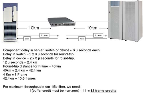
In the case of the switches I am using (HP FC16 switches), there is a port setting known as portCfgLongDistance, which can be set to one of three values: 0 = up to 10Km, 1 = up to 50Km, or 2 = 100Km. You need to check a number of things before setting this:
There is usually a Long Distance setting (similar to above) for the entire switch. This will require you to disable the switch before changing the setting.
Which ports can be set for Long Distance? Some switches group a number of consecutive ports onto a single ASIC (Application Specific Integrated Circuit) known as a loom. If we have four ports per loom, I would normally only be able to configure one port per loom as a Long Distance Port.
Configure all switches in the Fabric as Long Distance; otherwise, the Fabric will become segmented.
To increase BB_Credits is very seldom free; if you can afford long runs of fibre, then you can afford to pay the switch supplier for some more buffer credits. Remember to install the Long Distance license on all switched in the Fabric.
As you can see, long distances causes some configuration changes, and having ports communicating over +10Km will require an increase in your BB_Credits allowance on all your switches. The costs don't stop there.
We have been discussing the possibility of running Fibre Channel over distances up to and in excess of 10Km. This requires one fundamental piece of hardware: fibre-optic cable. I was talking to a customer in the UK recently who was considering running a private fibre over a distance of 30Km. The cost he was quoted for simply installing the fibre was approximately $7.5 million. That was for two individual fibres running in the same underground conduit. The customer immediately pointed out that having both fibres in the same conduit was not the best idea from a High Availability standpoint. To install two separate fibres was going to at least double the cost. Allied with this is the problem of access. You will need to gain access to the land you intend to run the fibre through. This can a considerable additional cost in terms of paying for access rights as well as the legal fees to administer such an undertaking. As you can imagine, few customers are laying their own fibre. The UK has an abundance of TV-cable companies that have taken the time, effort, and expense to lay fibre-optic cable all over the country. Lots of this fibre has no light signal going through it. This is known as dark fibre, simply because of the fact no light pulses are being sent down the fibre. As we have just discussed, laying your own fibre is expensive. Companies that have dark fibre are keen to recoup their investment costs. One way they can do this is to sell or lease you capacity on a dark fibre. If you wanted the bandwidth capabilities of an entire fibre all to yourself, I am sure they would charge you handsomely for the privilege. A common solution is to multiplex multiple optical frequencies down a fibre (using a standby fibre is a good idea for High Availability reasons) allowing multiple signals potentially from multiple sources to take advantages of the bandwidth potential of fibre. This solution is known as Dense Wave Division Multiplexing (DWDM). This solution involves leasing space or actually a frequency on a fibre from a telecom supplier. To attach to the fibre, you will connect through a DWDM device. The DWDM device may be housed on your site, or you may have to run fibre to the DWDM device itself. Either the telecom supplier or the DWDM supplier will normally ensure that the DWDM ports are installed and configured with appropriate converters for your type of connection: high speed converters for Fibre Channel, low speed converters for 100BaseFX Ethernet). The connections between the DWDM devices will be via long-wave GBICs over single-mode fibre. It's probably a good idea to ensure that as part of your agreement the telecom supplier is providing a redundant link in case a single cable fails. With more and more customers wanting to shift data long distances using Fibre Channel, lots of people have regarded DWDM as solely a feature of Fibre Channel SANs. It has become associated with Fibre Channel purely out of market forces. There is nothing to stop an organization running IP protocols over a DWDM link; it can support multiple protocols simultaneously. The great thing about using a DWDM device is that in a SAN it is simply seen as an extension port, an E_Port. This means we can plug a switch, a node, or even a storage device port directly into our DWDM device and visualize it as if we would any other switch in the Fabric. Well, almost. Once we start thinking about these kinds of distances, we need to start thinking about propagation delays. The DWDM devices will normally have huge bandwidth potential, but no matter how much data they can handle, they will introduce propagation delays due to internal circuitry as well as delays due to the length of the fibre they are attached to. Figure 23-7 above started the discussion regarding propagation delays in relation to BB_Credits. We also need to consider the propagation delays in regard of actual time scales. Let's look at an example:
We have a pair DWDM devices from a reputable manufacturer such as CNT (http://www.cnt.com → UltraNet Wave Multiplexer) or ADVA Optical (http://www.advaoptical.com → ADVA FSP-II). The latency from the single DWMD device is something approaching 250 nanoseconds = 2 x 250 ns = 500 ns latency.
Light in fibre travels at 200.000Km/second which equates to a latency = 5 ns.
A 50Km fibre = 50.000 * 5 ns = 250.000 ns latency.
Most applications, e.g., disk writes require a confirmation of the write, hence, the total latency is doubled.
Latency = 2 × ((250 ns × 2) + (50.000 × 5 ns)) = 0.501 ms
This is simply the latency introduced by the DWDM devices and the 50Km of fibre. We also need to consider any additional latency in connecting our servers and devices into our SAN. Such figures need to be considered when configuring software such as remote data replication software, which commonly has timeout values associated with getting a response from remote devices. DWDM links have been seen to run successfully over 10s of kilometers, in some cases up to 100Km. If distances beyond this are required, we may need to consider other solutions.
Once we go beyond what we could call metropolitan distances, we need to consider utilizing other wide area network (WAN) solutions. These will be supplied by telecom suppliers in the form of access to a high bandwidth network such as ATM. We will need to provide some hardware to connect to such a network. This device will be our bridge from Fibre Channel to the WAN; it will take Fibre Channel frames and break them up into ATM frames, reassembling them at the remote location. In our picture of our SAN, these ports will be seen as B_Ports. Companies such as CNT (http://www.cnt.com) provide products that perform such a task. For extended Cluster solutions, you will need to check with Hewlett-Packard which combinations of products are currently supported (CNT and CISCO are high on this list). The configuration of the bridge is normally within the remit of the supplier and/or the telecom company. We need to ensure that we have adequate bandwidth over the link and that we have paid for redundancy should there be a problem with connections to the WAN itself. Most bridge devices offer high availability features such as hot-swappable components and redundant internal devices. We should consider the possibility of such a device suffering a catastrophic failure itself. If we want to maximize the uptime of this solution, we may need to either (a) buy multiple bridges or (b) lease connections on bridges supplied by telecom suppliers and ensure that our contract stipulates 100 percent availability. These solutions are never cheap, and the cost increases exponentially with the bandwidth we require. Our bandwidth requirements will depend on the types of applications we are running over the link. Providing high-definition video (≈150MB/second) over a T1 link is not going to provide adequate performance. Knowing what solutions your telecom supplier is offering and at what cost is important. Here are some bandwidth figures for common WAN solutions:
Service (US telecom) | Link Speed |
|---|---|
DS1/T1 | 1.544 Mb/second |
DS3/T3 | 54 Mb/second |
OC-3c | 155 Mb/second |
OC-12c | 622 Mb/second |
OC-48c | 2.5 Gb/second |
OC-192c | 10 Gb/second |
Service (USA telecom) | Link Speed |
|---|---|
E1 | 2.048 Mb/second |
E3 | 34 Mb/second |
STM-1 | 155 Mb/second |
STM-4 | 622 Mb/second |
STM-16 | 2.5 Gb/second |
STM-64 | 10 Gb/second |
Although these figures look exciting, we need to consider two things:
The data rate (sometime called payload rate), which excludes any network-related headers, is commonly considerably less than the link speed, e.g., the data rate for STM-64/OC-192c ≈ 8.6 GB/second.
Know how much bandwidth you really need. How much data do you need to shift and in what timescale? If you need to perform a backup of 6TB of data in less than 24 hours, you will need at least an OC-12c/STM-4 connection. This is simple to calculate:
— OC-12c/STM-4
= 620 Mb/second
= 77,5 MB/second
= 279.000 MB/hour (≈272,5 GB/hour)
= 6.540 GB/day (≈6,4TB/day)
The propagation delay will not change just because you have more bandwidth. Do not be fooled by the telecom salespeople who want to throw bandwidth at the problem. You might have loads of bandwidth, but it is simply the latency involved in sending the data thousands of miles; to get from London to New York (approximately 4000 Km/ 2500 miles) takes 20ms one way. This means that if you are doing a disk IO from your Fifth Avenue apartments to a disk drive in your London office, you will experience a 40ms delay in getting a confirmation from the disk that the IO actually happened. There is nothing you can do about that unless you can break the speed of light.
When considering extending our SAN over long distances, it is normally to provide access to devices in remote sites. Although performing backups to tape devices hundreds of miles away is a possibility, most distance solutions are implemented for High Availability or Disaster Contingency considerations. It is common these days to replicate data from one disk to another disk at some distant location. In this way, if our local data center is wiped out by some natural disaster, we have access to our data from our remote disks. Hewlett-Packard's XP (eXtended Platform) disk array in conjunction with the software Continuous Access XP (a license key is entered on the XP disk array to unlock the functionality) is commonly used in this scenario. Other disc array manufacturers offer similar solutions; EMC Symmetrix with SRDF is one example. A concern we need to bear in mind when implementing these solutions is the question of distance. When performing IO between disks on remote sites, we can either perform the IO synchronously; both disks are guaranteed to have the same data or asynchronously; both disks might never have the same data. Figure 23-8 attempts to show the difference in IO behavior between synchronous and asynchronous data replication.
Continuous Access XP similarly has two modes (and two licenses) of operation with replication being performed on a LUN-by-LUN basis; different LUNs can use different modes of Continuous Access as long as both licenses are installed. The two modes for Continuous Access XP are Synchronous and Extended (=Asynchronous). The use of either synchronous or asynchronous IO is based on the desire or need to maintain data consistency and currency. There is a subtle difference between consistency and currency, so understanding that difference is important:
Consistency: This is where we are confident that the data on two physically separate but paired disks is of the same structure and format, and if we were to apply application logic to the data, we would achieve consistent results.
Currency: This is where the data on two physically separate but paired disks is the same in terms of content. If we were to extract any data record from one disk, currency dictates that the same data record exists on the second disk.
Whichever software and/or hardware tools you use to achieve offsite data replication, it is important that you understand their limitations (if any) in the area of offering data consistency and currency:
Continuous Access XP Synchronous is intended to be used where offsite data replication is required, and for data integrity reasons, we need to achieve both data consistency and currency. The issue here is when the IO from a server is confirmed by the disk array. In synchronous mode, the local XP will not acknowledge the IO until it has replicated the data onto the remote XP. Only at that time do we know that the XPs are synchronized and the IO can be confirmed back to the server. An issue here is that the link from one site to another must not incur too much of a latency; otherwise, the perceived IO performance for the application becomes unacceptable. With distance beyond 100Km, we can no longer look at using DWDM as an inter-switch link device; we need to start looking at WAN solutions mentioned previously. Remember, latency is not only the latency of the inter-site connection but also the latency of all the components between an end user and the user's data. Testing of perceived application performance and latency must be an end-to-end test.
Continuous Access XP Extended (=Asynchronous) is intended to be used where we have extended distances involved (hence the name). As discussed above, no matter how fat your pipe is (the amount of bandwidth), we will incur proportionally larger latencies as the distance we need to send the IO increases. The idea with Continuous Access XP Extended is that the local XP will confirm the IO back to the host server immediately. As soon as it can, but at some time later, the local XP will offload these IOs (in the correct sequence) to the remote XP. The IOs waiting to be sent over the remote link are stored in cache, so the busier the XP is with normal IO operations, the longer it may take to offload the pending IOs to the remote XP. Consequently, customers are strongly advised to double the amount of cache in both XPs; that's not a cheap solution. The asynchronous nature of IOs in this solution means we can say that Continuous Access XP Extended offers data consistency but not currency. In fact, with CA Extended we can be absolutely sure that the two XPs are current only by temporarily splitting the relationship between a PVOL and an SVOL. This flushes all pending IOs to the remote XP ensuring that they are current. Some customers never split a pair in this way, because while split you are storing up more and more pending IOs on your main XP disc array; you are increasing the level of non-currency between both sites. However, this splitting of a pair of PVOL and SVOL does mean we know that at the time of the split we can guarantee the PVOL and SVOL are current. This is sometimes performed so that we can take a current snapshot of the SVOL on the remote site. This is achieved by performing an internal copy of the LUN that can be used for backup, training, testing, or development purposes. The idea of splitting a pair of PVOL and SVOL is normally integrated into a sequence of tasks surrounding the host applications, i.e., having a quiescent database or performing an online database checkpoint, if possible. Once this snapshot has been taken, we can resynchronize the PVOL/SVOL pair.
Business Copy XP is an additional software key for an XP disc array. Business Copy XP has nothing to do with replicating data between two separate, distant XP disc arrays. Business Copy XP is a mechanism of taking an internal copy of a disk (a LUN) for backup, training, or testing purposes. It is commonly used in conjunction with Continuous Access XP to provide a backup copy of a LUN in both the local and remote sites.
A Continuous Access link from one XP to another is a unidirectional connection. Data travels from the Main Control Unit (MCU = main XP) to the Remote Control Unit (RCU = remote XP). This will normally be at least two physical fibre connections to avoid an SPOF and to ensure that data is transmitted in the most timely fashion. If you are looking to provide two-way failover, i.e., should the main site recover after a failure and the remote site faces a catastrophic failure, either an administrator will have to take the time to reconfigure the existing connections from MCU to RCU and vice-versa or to have in place additional unidirectional connections that allow the remote XP to replicate back to the MCU. This needs to be considered very carefully. This will require additional Fibre Channel connectors (called CHIP ports = Client Host Interface Port) on the XP as well as physical connections between the sites—a costly venture. This idea of being able to fall back from either side of the connection is commonly known as mutual recovery, the ability for either site to fall back to its partner site.
The use of extended SANs as well as synchronous/asynchronous data replication in High Availability Clusters is common. By installing additional software components, we will be able to manage the automatic/semi-automatic access to remote replicated data via a Serviceguard package. There are three software components aimed at such solutions: Extended Serviceguard Cluster, Metrocluster, and Continentalclusters. We discuss these solutions in Chapter 28.
If you are looking for more information relating to becoming certified in Fibre Channel, contact an organization called SNIA (Storage Network Industry Association), which will inform you of the process. It is not easy or straightforward; see http://www.snia.org for more details.
Virtual LAN (VLAN) technology allows us to separate logical network connectivity from physical connectivity. This concept is different from a traditional LAN in that a LAN is limited by its physical connectivity. All users in a LAN belong to a single broadcast domain[1] and can communicate with each other at the Data Link layer or Layer 2 of the OSI seven-layer model. Network managers have used LANs to segment a complex network into smaller units for better manageability, improved performance, and security. For example, network managers use one LAN for each IP subnet in their network. Communication between subnets is made possible at the Network Layer or Layer 3, using IP routers. A VLAN may be thought of as a single physical network that can be logically divided into discrete LANs that can operate independent of each other.
To implement a VLAN in your network, you must use VLAN-aware switches. In order to understand how logical partitioning of a LAN infrastructure is done using VLAN, you should remember the fundamental operation of a traditional switched LAN. Without going into too much detail of switch design, you should remember two simple rules regarding the functioning of a regular LAN switch:
When the switch receives a broadcast or multicast frame from a port, it floods (broadcasts) the frame to all other ports on the switch.
When the switch receives a unicast frame, it forwards it only to the port to which it is addressed.
A VLAN-aware switch changes the above two rules as follows:
When the switch receives a broadcast or multicast frame from a port, it floods the frame only to those ports that belong to the same VLAN as the frame.
When a switch receives a unicast frame, it forwards it to the port to which it is addressed only if the port belongs to the same VLAN as the frame.
A unique number called the VLAN ID identifies each VLAN. It is a 12-bit field in the VLAN tag. Therefore, you can have a theoretical maximum of 4095 discrete VLANs in your network.
VLAN-aware switches can be configured to add ports to a VLAN group or groups. They maintain two simple, related tables: 1) a list of ports that belong to each VLAN enabled on the switch, and 2) the set of VLANs enabled on each port. The most basic VLAN-aware switches support port-based VLANs, meaning that the switch port on which the frame arrived determines the VLAN membership of the frame. These switches cannot support more than one VLAN per switch port, unless they support VLAN tagging, which is explained later. As you see later, a simple port-based VLAN that supports VLAN tagging is all that is needed to implement a VLAN in an HP-UX environment. More sophisticated switch offerings allow users to configure VLAN membership rules based on frame content such as MAC address, TCP/UDP port, IP address, and so on. But doing this may affect switch performance. VLAN-aware Layer 3 switches (or Routing Switches) will perform the function of Layer 3, e.g., IP routing in addition to VLAN classification.
As mentioned previously, VLAN functionality may also be implemented via explicit frame tagging by end stations or switches. The end station or switch determines the VLAN membership of a frame and inserts a VLAN tag in the frame header, so that downstream link partners can examine just the tag to determine the VLAN membership. Devices that can classify frames by inspecting their VLAN tags are called tag-aware. Tagging has several advantages—VLAN association need be applied only once at an end station or at an edge switch, so that downstream switches all the way to the destination are relieved of the burden of classifying frames. Tagging at end stations is particularly attractive because the overhead of frame classification is distributed.
IEEE 802.1Q specifies the architecture for VLAN tagging: tag format, tag insertion, and tag stripping. The IEEE 802.1Q tag also has a provision for priority encoding. The 3-bit “PRI” bit is the tagged frame priority information. IEEE 802.1p (later incorporated in IEEE 802.1D) has standardized this priority encoding.
Switches that implement only port-based VLAN can support only one VLAN per port. However, if they are tag-aware (also called Q-compliant), they could support multiple VLANs per port: one untagged VLAN and multiple tagged VLANs. If a frame doesn't have an explicit VLAN tag, it is automatically assigned the untagged VLAN ID or the default VLAN ID. An inbound frame that is tagged has its VLAN ID in the frame header. Some switch vendors refer to the ability of handling multiple tagged frames per port as VLAN trunking.
HP-UX supports three types of VLANs, port-based, protocol-based, and IP subnet-based:
port-based VLAN: All frames transmitted by a NIC are tagged using one and only one VLAN ID. The NIC doesn't transmit or receive any untagged frames.
protocol-based VLAN: The NIC assigns a unique VLAN ID for each Layer 3 protocol (e.g., IPv4, IPv6, IPX, and so on). In other words, the VLAN ID of outbound frames is different for different protocols. An inbound frame is dropped if the protocol and VLAN ID don't match.
IP subnet-based VLAN: The NIC assigns a unique VLAN ID for each IP subnet it belongs to. In other words, the VLAN ID of outbound frames is different for different destination subnets. An inbound frame is dropped if the IP subnet and VLAN ID don't match.
HP-UX implements VLAN tagging via a mechanism called virtual interfaces (VIs). On each NIC port, you may configure multiple VIs, each of which is associated with a unique VLAN ID and 802.1p priority value. Each VI is assigned a virtual PPA (Physical Point of Attachment), which can then be used just like any other PPA—for configuring protocols or attaching to applications, and so on.
The software is available to download free of charge from http://software.hp.com/portal/swdepot/displayProductInfo.do?productNumber=VLAN. Currently, it is supported only on HP-UX 11i version 1.0. Figure 23-9 shows a typical VLAN configuration:
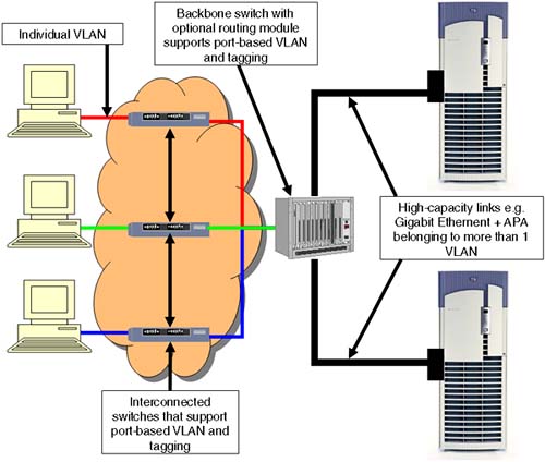
A virtual private network is a secure communication channel constructed within the framework of a public network infrastructure. The term virtual private network refers to a private network that is physically deployed across a public network, such as the Internet. The term virtual implies a logical network, as opposed to a physical dedicated network. The term private network implies that the communication among the users is confidential and cannot be seen by others, similar to a dedicated leased-line situation. A VPN provides the same benefits as a dedicated leased-line (privacy), without having to pay for a leased line (companies can use the Internet).
A well-secured network environment contains three critical security elements:
Barriers: Barriers limit access to the systems and networks based on filter conditions. Often referred to as firewalls, barriers limit access based on IP addresses, port addresses, protocol types, usernames, or passwords.
Encryption: Encryption prevents eavesdroppers from viewing network traffic as it travels between the source and destination systems. Encryption is needed to guarantee data integrity and privacy.
Intrusion: Intrusion detection tools continually monitor to determine if someone has gained or is trying to gain unauthorized access to the system. Intrusion detection tools are the sensors that alert IT managers when security access violations occur.
Three key technologies used in providing VPN solutions include but are not limited to:
IPsec/9000: Hewlett-Packard's IPSec product supports elements for network security, such as confidentiality, authentication, integrity, non-repudiation, packet filtering, management, and administration with access control. The IPSec product is built on industry standards and is designed to provide interoperable, high quality, cryptographically based security for IP packet traffic. IPSec addresses these security problems:
Packet tampering
Spoofing
Capture of critical data, such as passwords and credit card numbers, sent over the network in clear text
IPSec provides a secure encrypted user session between two end-systems running HP-UX. IPSec does not adversely affect other users, hosts, or Internet components that do not employ IPSec to protect their traffic.
IPFilter: HP-UX IPFilter (B9901AA) is a stateful system firewall that filters IP packets to control packet flow in or out of a machine. It works as a security defense by cutting down on the number of exposure points on a machine.
HP-UX IPFilter is based on ipfilter v3.5 alpha 5 from the open source community (see http://caligula.anu.edu.au/~avalon/ for more detail). It can be run either as DLKM or as statically linked modules. These are the key benefits of IPFilter:
It allows control of incoming TCP connections through the Dynamic Connection Allocation (DCA) feature.
It supports the Network Address Translation (NAT) feature, which lets an intermediate HP-UX system act as a translator of IP addresses and network ports.
It explicitly permits or denies a packet from passing through, based on the following:
It sends back ICMP error/TCP reset for blocked packets.
It keeps packet state information for TCP, UDP, and ICMP.
It keeps fragment state information for any IP packet, applying the same rule to all fragments.
It drops all fragmented traffic if specified by rule.
It redirects packets for forensic analysis if specified by rule.
It creates extensive logs when required.
HP-UX AAA Server: The HP-UX AAA Server is used for Authentication, Authorization, and Accounting of user network access at the entry point to a network. The HP-UX AAA Server provides user authentication for network access devices by utilizing the industry standard Remote Authentication Dial-In User Service (RADIUS) protocol. This product also provides RADIUS-based authorization and accounting (access) log files that can be used by billing and accounting applications. A key feature for enterprise-wide authentication is the support for LDAP version 3 compliant directories as well as Oracle databases.
We look at both IPSec and IPFilter in detail in Chapter 30, “A New Breed of Security Tools.” A key feature of a VPN is to ensure that all communications over any external networks (the Internet) are kept private. Public-key cryptography is a key element in such a design. Keys need to be distributed in such as way as to be secure as well as accessible. Within an organization, an LDAP server within the DMZ of the organization can provide a mechanism whereby corporate-wide information (the public keys of the partners you are communicating with) is made available to everyone within the organization. This avoids internal clients having to access the Internet to obtain public keys for remote partners. External to the corporation, Certification Authorities will manage the distribution and secure handling of each organization's public keys. A full discussion of PKI (Public Key Infrastructure) is handled in Chapter 30. As always, http://docs.hp.com provides an invaluable source of information on all these topics. Figure 23-10 shows a stylized view of a possible VPN solution. NOTE: Not all devices are shown in the name of simplicity.
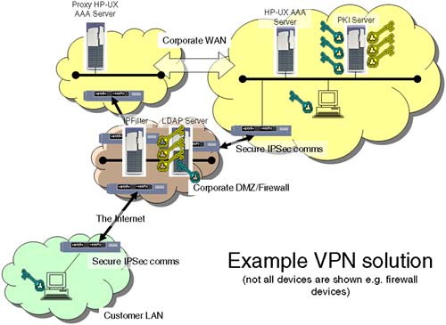
In this chapter, we have looked at a number of network technologies that are becoming more and more common in the corporate network infrastructure. Most of these technologies are used in long-haul data communications: everything from WAN solutions, to Fibre Channel, and finally two technologies to offer traditional IP solutions but utilizing virtual technologies—VLAN and VPN. We have not gone into great depth with any of these subjects because each commands an entire book of its own. What we have done is to highlight their key features, benefits, and costs! Being a CSE, you may come across these technologies, and it is an appreciation of these technologies that we are aiming for in this chapter. Further study will be necessary should additional hands-on information be required. During our discussions, I have tried to point you to additional sources of information as well as to http://docs.hp.com. This concludes our discussion on Other Network Technologies.
[1] A LAN is a broadcast domain at the Data Link Layer because a broadcast or multicast frame sent from a station is seen by all other stations in its LAN.