
Chapter 8. Why the Diagramming Method Works
It is well to moor your bark with two anchors.
Chapter 5-Chapter 7 covered how to tune SQL with the diagramming method but did not discuss why the method leads to well-tuned SQL. With a lot of faith and good memory, you could likely get by without knowing why the method works. However, even with unbounded, blind faith in the method, you will likely have to explain your SQL changes occasionally. Furthermore, the method is complex enough that an understanding of why it works will help you remember its details better than blind memorization ever could.
The Case for Nested Loops
Throughout this book, I have asserted that nested-loops joins on the join keys offer more robust execution plans than hash or sort-merge joins. Let’s examine why. Consider a two-table query diagram, as shown in Figure 8-1.
Sight-unseen, it is possible to say a surprising amount about this query, to a high probability, if you already know that it is a functionally useful business query that has come to you for tuning:
The top table, at least, is large or expected to grow large. Because Jd, the detail join ratio, is greater than 1.0 (as is usual), the bottom table is smaller than the top table by some factor, but that factor could be moderate or large. Queries that read only small tables are common enough, but they rarely become a tuning concern; the native optimizer produces fast execution plans without help when every table is small.
Large tables are likely to grow larger with time. They usually became large in the first place through steady growth, and that growth rarely stops or slows down.
The query should return a moderate number of rows, a small fraction of the number in the detail table. Certainly, queries can return large rowsets, but such queries are usually not useful to a real application, because end users cannot effectively use that much data at once. Online queries for a real application should generally return fewer than 100 rows, while even batch queries should usually return no more than a few thousand.
While tables grow with time, the inability of end users to digest too much data does not change. This often means that the query conditions must point to an ever-decreasing fraction of the rows in the larger table. Usually, this is achieved by some condition that tends to point to recent data, since this tends to be more interesting from a business perspective. Although a table might contain an ever-lengthening history of a business’s data, the set of recent data will grow much more slowly or not at all.
The number of rows the query returns is Ca x Fa x Fb, where Ca is the rowcount of table
A.
These assertions lead to the conclusion that the product of the two filter ratios (Fa x Fb) must be quite small and will likely grow smaller with time. Therefore, at least one of Fa and Fb must also be quite small. In practice, this is almost always achieved with one of the filter ratios being much smaller than the other; the smaller filter ratio is almost always the one that grows steadily smaller with time. Generally, the smallest of these filter ratios justifies indexed access in preference to a full table scan.
If the best (smallest) filter ratio is Fb and it is low enough to justify indexed
access to table B, then nested loops
from B will generally point to the
same fraction (Fb) of rows in table
A. (A given fraction of master
records will point to the same fraction of details.) This fraction will
also be low enough to justify indexed access (through the foreign key,
in this case) to table A, with lower
cost than a full table scan. Since Fb<Fa
under this assumption, nested loops will minimize the number of rows
touched and therefore minimize the number of physical and logical I/Os
to table A, compared to an execution
plan that drives directly through the index for the filter on A. Either a hash or a sort-merge join to table
A would require a more expensive full
table scan or index range scan on the less selective filter for table
A. Since index blocks for the join
are better cached than the large table A, they are inexpensive to read, by comparison
to table blocks. Therefore, when the best filter ratio is Fb, nested loops minimize the cost of the
read to table A.
When the best filter is on the detail table (table A, in this case), the same argument holds at
the limit where Jd=1. When
Jd>1, larger values of Jd tend to favor hash joins. However, unless Jd is quite large, this factor does not
usually overcome the usually strong advantage of driving to every table
from the most selective filter. When Jd is large, this implies that the master
table B is much smaller than the
detail table A and will be
consequently much better cached and less expensive to reach, regardless
of the join method. I already discussed this case at length in Section 6.6.5 in Chapter 6, and I won’t repeat it all
here. The key point is that, even in the cases in which hash joins
improve a given join cost the most, they usually reduce only a
comparatively minor component of the query cost—the cost of reaching a
much smaller, better-cached master table. To achieve even this small
benefit, the database must place the joined-to rowset in memory or,
worse, store the hashed set temporarily on disk.
Choosing the Driving Table
The most important choice you make when putting together an execution plan is your choice of the driving table. You will rarely find a good execution plan without driving from the single best choice, and the best choice of driving table usually ensures at worst a pretty good plan, even if you pick the remainder of the join order quite haphazardly. I’ve stated that the rule for choosing the best driving table is simple: just drive from the table with the lowest filter ratio. Here, I make the case that such a simple rule almost always works and is really the only possible rule that is both simple and usually right.
The dilemma for all optimizers, human or otherwise, is how to choose the best driving table without iterating through every join order or even a significant fraction of the join orders. Any fast method for choosing the driving table must depend on localized information—information that does not reflect the entire complexity of the query. To demonstrate the reasoning behind the simple rule to drive from the table with the lowest filter ratio, I discuss a problem with deliberately hidden details, hiding the full complexity of the query. Consider the partially obscured query diagram of Figure 8-2.
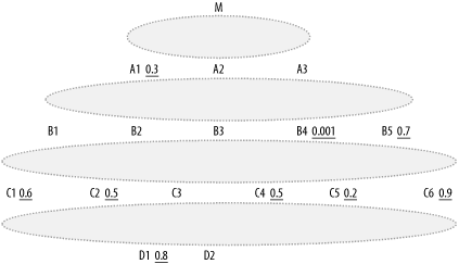
What does such a diagram convey, even in the absence of the join links? Without the join links or join ratios, you can still say, with fair confidence:
Mis the root detail table, likely the largest and least-well-cached table in the query. Call the rowcount of this table C.A1,A2, andA3are master tables that join directly toM.All the other tables are also master tables and appear to be joined indirectly to
M, through intermediate joins.
Even with this sparse information, you can deduce a key property
of the cost of reading that largest and least-well-cached root detail
table M:
The number of rows read from the root detail table will be no more than that table’s rowcount (C) times the driving table’s filter ratio.
For example, even if table B4
holds the only filter you can reach before you join to M, driving from B4 with nested loops ensures that you read
just one-thousandth of the rows in M.
Figure 8-3 illustrates this
case.
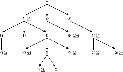
Of course, if B4 connects
directly to more nodes with filters before it must join to M, you can do even better. However, as long as
you choose nested-loops joins, you know immediately that the upper bound
of the cost of the read of the root detail table is C x Fd,
where Fd is the filter ratio for
the chosen driving table. This explains the driving-table rule, which
chooses the node with the lowest filter factor as the driving table. To drive home
this point, Figure 8-4
rearranges the links in Figure
8-3 to make a new diagram that maximizes the advantage of an
alternative to driving from B4.
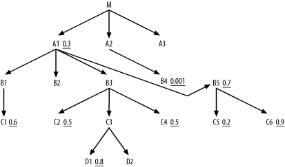
Now, if you drive from A1 or
any node connected below it, you can pick up every filter except the
filter on B4 before reaching M. The result is that you reach a number of
rows in M equal to C x 0.0045 (C x 0.3 x 0.7 x 0.6 x 0.5 x 0.5 x 0.2 x 0.9 x
0.8), which is over four times worse than the cost of driving from
B4. Furthermore, with a poor initial
driving filter, the other early-table access costs will also likely be
high, unless all those tables turn out to be small.
You might wonder whether this example is contrived to make the best driving filter look especially good, but the contrary is true: most real queries favor driving from the lowest filter ratio even more dramatically! Most queries have far fewer filters to combine, and those filters are more spread out across different branches under the root detail table than they are in this example. If you had two almost equally good filters, you could build a plausible-looking case for driving from the second-best filter if it had more near-neighbor nodes with helpful filters as well, such as in Figure 8-5.
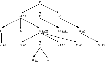
In this contrived case, B3
would likely make a better driving node than B4, since B3 receives so much help from its neighboring
nodes before you would join to M.
This might sound like a plausible case, and I don’t doubt it can occur,
but empirically it is rare. I haven’t seen a case such as this in 10
years of tuning, mainly because it is so rare to find two very selective
filters with roughly the same magnitude of selectivity in the same
query. It is much more common that most of the selectivity of a query
comes from a single highly selective condition.
Choosing the Next Table to Join
After you choose the driving table, the rest of the decisions for a robust execution plan consist of a series of choices amounting to “What’s next?” When you ask this question, you have, effectively, a single cloud of already-joined nodes that you chose earlier in the join order and a series of nodes linked to that cloud that are eligible for the next join. If the query diagram is a typical tree structure, at most one node will be upward from the current cloud, and any number of nodes can be reachable downward. Figure 8-6 illustrates this typical case.
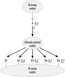
Consider the question “What’s next?” for this point in the join order. The database has reached some number of rows, which I will call N. Joins to tables downward of the current join cloud will multiply the running rowcount by some fraction: the filter ratio times the master join ratio. Let F=R x M, where R is the filter ratio and M is the master join ratio (which is 1.0, unless shown otherwise). The larger the reduction in rows, which is 1-F, the lower the cost of the future joins, so nodes with high values of 1-F have high value to optimizing the rest of the query, when joined early. That reduction in rowcount has a cost too, based on the cost per row driving into the join, which I will call C. The benefit-to-cost ratio of a downward join under consideration is then (1-F)/C. If you assume a uniform cost per row read for all tables downward of the already-joined nodes, choosing the downstream node with the maximum value of (1-F)/C is the same as choosing the node with the minimum value of F.
How could this optimization be refined further? There are three opportunities for improvements, all reflected in Section 6.6 in Chapter 6:
Not all downstream nodes have equal cost per row joined, so C really does vary between nodes.
The full payoff for a join is sometimes not immediate, but comes after joining to nodes further downstream made accessible through that intermediate join.
Sometimes, the upstream node actually offers the best benefit-to-cost ratio, even while downstream nodes remain.
I will discuss these improvement opportunities one at a time to illustrate how they create the special rules that occasionally override the simpler rules of thumb.
Accounting for Unequal Per-Row Costs
Downstream nodes are nearly guaranteed to be smaller than the largest table already reached in the execution plan. As such, they are generally better cached and unlikely to have deeper indexes than the largest table already reached, so their impact on overall cost is typically minor. Even when the costs of reading downstream nodes vary considerably, the performance cost of assuming uniform costs for these nodes usually is minor compared to the overall costs of the query. Nevertheless, the possibility of significant join cost differences justifies the exception already mentioned in Chapter 6:
Prefer to drive to smaller tables earlier, in near-ties. After you choose the driving table, the true benefit-to-cost ratio of joining to the next master table is (1-F)/C. Smaller tables are better cached and tend to have fewer index levels, making C smaller and making the benefit-to-cost ratio tend to be better for smaller tables.
Accounting for Benefits from Later Joins
Occasionally, especially when nodes have no filter at all, the greatest benefit of a join is that it provides access to a further-downstream node that has a good filter. This gives rise to another exception described in Chapter 6:
In the case of near-ties, prefer to drive to tables earlier that allow you to reach other tables with even better filter ratios sooner in the execution plan. The general objective is to discard as many rows as soon in the execution plan as possible. Good (low) filter ratios achieve this well at each step, but you might need to look ahead a bit to nearby filters to see the full benefit of reaching a given node sooner.
A perfect account of these distributed effects of filters spread across nodes is beyond the scope of this book and beyond any optimization method meant for manual implementation. Fortunately, this limitation turns out to be minor; I have never seen a case when such a perfect account was necessary. Almost always, the preceding rough rule delivers a first solution that is optimum or close enough to optimum not to matter. Rarely, a little trial and error is worth trying when a case is right on the borderline. Such rarely needed trial and error is far easier and more accurate than the most elaborate calculations.
When to Choose Early Joins to Upstream Nodes
Upstream nodes can potentially offer the most effective benefit-to-cost ratio. For upstream nodes, you calculate F=R x D, where R is the node’s filter ratio, as before, and D is the detail join ratio. However, unlike the master join ratio, which must be less than or equal to 1.0, the detail join ratio can be any positive number and is usually greater than 1.0. When it is large, F is typically greater than 1.0 and the benefit-to-cost ratio, (1-F)/C, is actually negative, making the upward join less attractive than even a completely unfiltered downward join (where 1-F is 0). When F is greater than 1.0, the choice is obvious: postpone the upward join until downward joins are exhausted. Even when the detail join ratio (D) is small enough that F is less than 1.0, an early upward join carries a risk: the detail join ratio might be much larger for other customers who will run the same application, or for the same customer at a later time. The early upward join that helps this one customer today might later, and at other sites, do more harm than good. Upward joins are not robust to changes in the data distribution.
Large detail join ratios carry another, more subtle effect: they point to large tables that will require the database to read multiple rows per joined-from row, making C higher by at least the detail join ratio, just to account for the higher rowcount read. If these upstream tables are particularly large, they will also have much larger values for C (compared to the downstream joins), owing to poorer caching and deeper indexes. Together, these effects usually make C large enough that the benefit-to-cost ratio of an upstream join is poor, even with very low detail-table filter ratios.
In Figure 8-6, the
factor (F) for A is 0.2 (0.1 x 2), the same as the best
downstream node, B3, but the cost
(C) would be at least twice as
high as for any downstream node, since the database must read two rows
in A for every joined-from row from
the already-joined nodes. Setting Cd (the detail-table per-row cost) equal to
2 / Cm (the worst-case per-row
cost of a master-table join) gives you (1-0.2)/(2 x Cm) = (1-Fe)/Cm, where Fe is the filter ratio a worst-case
downstream join would have if it had a benefit-to-cost ratio equal to
the upstream join to A. Solving for
Fe, you find 1-Fe=0.8/2, or Fe=0.6.
Based on this calculation, you would certainly choose the joins to
B3, B4, and B2 before the join to A. Even the join to B5 would likely be best before the join to
A, since B5 would likely be better cached and have
fewer index levels than A. Only the
join to B1 would be safely
postponed until after the join to A, if you had confidence that the F factor for A would never exceed 1.0 and you had no
further filters available in nodes downstream of B1. By the time you reach a point where the
upward join might precede a downward join, it often hardly matters,
because by that point there are so few rows left after the earlier
filters that the savings are miniscule compared with the costs of the
rest of the query. In conclusion, the need even to consider upward
joins early, with any detail join ratio of 2 or more, is
slight.
However, detail join ratios are sometimes reliably less than 1.0, leading to the simplest exception to the rule that you should not consider upward joins early:
When choosing the next node in a sequence, treat all joins with a join ratio D less than 1.0 like downward joins. And, when comparing nodes, use D x R as the effective node filter ratio, where R is the single-node filter ratio.
When detail join ratios are near 1.0 but not less than 1.0, the case is more ambiguous:
Treat upward joins like downward joins when the join ratio is close to 1.0 and when this allows access to useful filters (low filter ratios) earlier in the execution plan. When in doubt, you can try both alternatives.
The key in this last case is how confident you are in the detail join ratio being close to 1.0. If it might be large later, or at another site, it is best to push the upward join later in the plan, following the simplest heuristic rule that postpones the upward joins until downward joins are complete. (Important exceptions to this rule are surprisingly rare.)
Summary
Short of a brute-force analysis of huge numbers of execution plans, perfect optimization of queries with many tables is beyond the state-of-the-art. Even with advances in the art, perfect optimization is likely to remain beyond the scope of manual tuning methods. If you make your living tuning SQL, this is actually good news: you are not about to be put out of business! The problem of SQL tuning is complex enough that this result is not surprising. What is surprising, perhaps, is that by focusing on robust execution plans and a few fairly simple rules, you can come close to perfect optimization for the overwhelming majority of queries. Local information about the nodes in a join diagram—in particular, their filter ratios—turns out to be enough to choose an efficient, robust execution plan, without considering the problem in its full combinatorial complexity.