
Every Access expert stocks his or her database with a few (or a few dozen) useful queries that simplify day-to-day tasks. In the previous chapter, you learned how to create queries that chew through avalanches of information and present exactly what you need to see. But as Access masters know, there’s much more power lurking just beneath the surface of the query design window.
In this chapter, you’ll delve into some query magic that’s sure to impress your boss, co-workers, and romantic partners. You’ll learn how to carry out calculations in a query and perform summaries that boil columns of numbers down to neat totals. You’ll also learn how to write super-intelligent filter expressions and how to create dynamic queries that ask for information every time you run them. These techniques are indispensable to the repertoire of any true query fanatic.
When you started designing tables, you learned that it’s a database crime to add information that’s based on the data in another field or another table. An example of this mistake is creating a Products table that has both a Price and a PriceWithTax field. The fact that the PriceWithTax field is calculated based on the Price field is a problem. Storing both is a redundant waste of space. Even worse, if the tax rate changes, then you’re left with a lot of records to update and the potential for inconsistent information (like a with-tax price that’s lower than a no-tax price).
Even though you know not to create fields like PriceWithTax, sometimes you will want to see calculated information in Access. Before Boutique Fudge prints a product list for one of its least-loved retailers, it likes to apply a 10 percent price markup. To do this, it needs a way to adjust the price information before printing the data. If the retailer spots the lower price without the markup, they’re sure to demand it.
Queries provide the perfect solution for these kinds of problems, because they include an all-purpose way to mathematically manipulate information. The trick’s to add a calculated field: a field that’s defined in your query, but doesn’t actually exist in the table. Instead, Access calculates the value of a calculated field based on one or more other fields in your table. The values in the calculated field are never stored anywhere—instead, Access generates them each time you run the query.
To create a calculated field, you need to supply two details: a name for the field, and an expression that tells Access what calculation it must perform. Calculated fields are defined using this two-part form:
CalculatedFieldName: ExpressionFor example, here’s how you can define the PriceWithTax calculated field:
PriceWithTax: [Price] * 1.10Essentially, this expression tells Access to take the value from the Price field, and then multiply it by 1.10 (which is equivalent to raising the price by 10 percent). Access repeats this calculation for each record in the query results. For this expression to work, the Price field must exist in the table. However, you don’t need to show the Price field separately in the query results.
You can also refer to the Price field using its full name, which is made up of the table name, followed by a period, followed by the field name, as shown here:
PriceWithTax: [Products].[Price] * 1.10This syntax is sometimes necessary if your query involves more than one table (using a query join, as described in Section 6.3), and the same field appears in both tables. In this situation, you must use the full name to avoid ambiguity. (If you don’t, Access gives you an error message when you try to run the query.)
Note
Old-time Access users sometimes replace the period with an exclamation mark (as in [Products]![Price], which is equivalent.
To add the PriceWithTax calculated field to a query, you need to use Design view. First, find the column where you want to insert your field. (Usually, you’ll just tack it onto the end in the first blank column, although you can drag the other fields around to make space.) Next, type the full definition for the field into the Field box (see Figure 7-1).
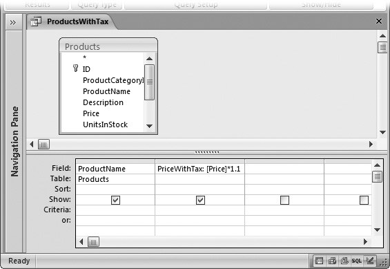
Figure 7-1. This query shows two fields straight from the database (ID and Name), and adds the calculated PriceWithTax field. The ordinary Price field, which Access uses to calculate PriceWithTax, isn’t shown at all.
Now you’re ready to run the query. When you do, the calculated information appears alongside your other columns (Figure 7-2). If you don’t like the fact that your calculated information appears in a slightly messier format—with more decimal places and no currency symbol—you can fix it up using the rounding (Section 7.2.1.1) and formatting (Section 7.2.3) features discussed later in this chapter.
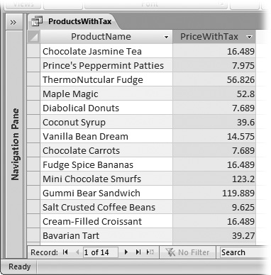
Figure 7-2. The query results now show a PriceWithTax field, with the result of the 10 percent markup. The neat part’s that this calculated information’s now available instantaneously, even though it isn’t stored in the database. Try and beat that with a pocket calculator.
Calculated fields do have one limitation—since the information isn’t stored in your table, you can’t edit it. If you want to make a price change, you’ll need to edit the underlying Price field—trying to change PriceWithTax would leave Access thoroughly confused.
Note
An expression works on a single record at a time. If you want to combine the information in separate records to calculate totals and averages, then you need to use the grouping features described in Section 7.3.
Before going any further, it’s worth reviewing the rules of calculated fields. Here are some pointers:
Always choose a unique name. An expression like Price: [Price] * 1.10 creates a circular reference, because the name of the field you’re using is the same as the name of the field you’re trying to create. Access doesn’t allow this sleight of hand.
Build expressions out of fields, numbers, and math operations. The most common calculated fields take one or more existing fields or hard-coded numbers and combine them using familiar math symbols like addition (+), subtraction (−), multiplication (*), or division (/).
Expect to see square brackets. The expression PriceWithTax: [Price] * 1.10 is equivalent to PriceWithTax: Price * 1.10 (the only difference is the square brackets around the field name Price). Technically, you need the brackets only if your field name contains spaces or special characters. However, when you type in expressions that don’t use brackets in the query Design view, then Access automatically adds them, just to be on the safe side.
Many calculated fields rely entirely on ordinary high school math. Table 7-1 gives a quick overview of your basic options for combining numbers.
You’re free to use as many fields and operators as you need to create your expression. Consider a Products table with a QuantityInStock field that records the number of units in your warehouse. To determine the value you have on hand for a given product, you can write this expression that uses two fields:
ValueInStock: [UnitsInStock] * [Price]
Tip
When performing a mathematical operation with a field, you’ll run into trouble if the field contains a blank value. To correct the problem, you need the Nz( ) function, which is described in Section 7.3.
You can also use the addition and subtraction operators with date fields. (You can use multiplication, division, and everything else, but it doesn’t have any realistic meaning.)
Using addition, you can add an ordinary number to a date field. This number moves the date forward by that many days. Here’s an example that adds two weeks of headroom to a company deadline:
ExtendedDeadline: [DueDate] + 14
If you use this calculation with the date January 10, 2007, the new date becomes January 24, 2007.
Using subtraction, you can find the number of days between any two dates. Here’s how you calculate how long it was between the time an order was placed and when it was shipped:
ShippingLag: [ShipDate] - [OrderDate]
If the ship date occurred 12 days after the order date, you’d see a value of 12.
Note
Date fields can include time information. In calculations, the time information’s represented as the fractional part of the value. If you subtract two dates and wind up with the number 12.25, that represents 12 days and six hours (because six hours is 25 percent of a full day).
Remember, if you want to include literal dates in your queries (specific dates you supply), you need to bracket them with the # character and use Month/Day/Year format. Here’s an example that uses that approach to count the number of days between the date students were expected to submit an assignment (March 20, 2007) and the date they actually did:
LateDays: [DateSubmitted] - #03/20/07#
A positive value indicates that the value in DateSubmitted is larger (more recent) than the deadline date—in other words, the student was late. A value of 4 indicates a student that’s four days off the mark, while –4 indicates a student that handed the work in four days ahead of schedule.
If you have a long string of calculations, Access follows the standard rules for order of operations: mathematician-speak for deciding which calculation to perform first when there’s more than one calculation in an expression. So if you have a lengthy expression, Access doesn’t just carry on from left to right. Instead, it evaluates the expression piece by piece in this order:
Suppose you want to take the QuantityInStock and the QuantityOnOrder fields into consideration to determine the value of all the product you have available and on the way. If you’re not aware of the order of operation rules, then you might try this expression:
TotalValue: [UnitsInStock] + [UnitsOnOrder] * [Price]
The problem here is that Access multiplies QuantityOnOrder and Price together, and then adds it to the QuantityInStock. To correct this oversight, you need parentheses like so:
TotalValue: ([UnitsInStock] + [UnitsOnOrder]) * [Price]
Now the QuantityInStock and QuantityOnOrder fields are totaled together, and then multiplied with the Price to get a grand total.
Tip
Need some more space to write a really long expression? You can widen any column in the query designer to see more at once, but you’ll still have trouble with complex calculations. Better to click in the Field box, and then press Shift+F2. This action pops open a dialog box named Zoom, which shows the full content in a large text box, wrapped over as many lines as necessary. When you’ve finished reviewing or editing your expression, click OK to close the Zoom box and keep any changes you’ve made, or Cancel to discard them.
Although calculated fields usually deal with numeric information, they don’t always. You have genuinely useful ways to manipulate text as well.
If you have text information, then you obviously can’t use addition, subtraction, and other mathematical operations. However, you can join text together. You can, for instance, link several fields of address information together and show them all in one field, conserving space (and possibly making it easier to export the information to another program).
To join text, you use the ampersand (&) operator. For example, here’s how to create a FullName field that draws information from the FirstName and LastName fields:
FullName: [FirstName] & [LastName]
This expression looks reasonable enough, but it’s actually got a flaw. Since you haven’t added any spaces, the first and last name end up crammed together, like this: BenJenks. A better approach is to join together three pieces of text: the first name, a space, and the last name. Here’s the revised expression:
FullName: [FirstName] &" "& [LastName]
This produces values like Ben Jenks. You can also swap the order and add a comma, if you prefer to have the last name first (like Jenks, Ben) for better sorting:
FullName: [LastName] & ", " & [FirstName]
Note
Access has two types of text values: those you draw from other fields, and those you enter directly (or hard-code). When you hard-code a piece of text (such as the comma and space in the previous example), you need to wrap it in quotation marks so Access knows where it starts and stops.
You can even use the ampersand to tack text alongside numeric values. If you want the slightly useless text “The price is” to appear before each price value, use this calculated field:
Price: "The price is: " & [Price]
By now, it may have crossed your mind that you can manipulate numbers and text in even more ambitious ways—ways that go beyond what the basic operators let you do. You may want to round off numbers or capitalize text. Access does include a feature that lets you take your expressions to the next level, and it’s called functions.
A function’s a built-in algorithm that takes some data that you supply, performs a calculation, and then returns a result. The difference between functions and the mathematical operators you’ve already seen is the fact that functions can perform far more complex operations. Access has a catalog with dozens of different functions, many of which perform feats you wouldn’t have a hope of accomplishing on your own.
Functions come in handy in all sorts of interesting places in Access. You can use them in:
Calculated fields. To add information to your query results.
Filter conditions. To determine what records you see in a query.
Visual Basic code. The all-purpose extensibility system for Access that you’ll tackle in Part Five.
As you explore the world of functions, you’ll find that many are well suited to calculated fields but not filter conditions. In the following sections, you’ll see exactly where each function makes most sense.
Note
Functions are a built-in part of the Access version of SQL (Section 6.2.3), which is the language it uses to perform data operations.
Whether you’re using the simplest or the most complicated function, the syntax —the rules for using a function in an expression—is the same. To use a function, simply enter the function name, followed by parentheses. Then, inside the parentheses, put all the information the function needs in order to perform its calculations (if any).
For a good example, consider the handy Round( ) function, which takes a fractional number and then tidies up any unwanted decimal places. Round( ) is a good way to clean up displayed values in a calculated field. You’ll see why Round( ) is useful if you create an expression like this, which discounts prices by five percent:
SalePrice: [Price] * 0.95
Run a price like $43.97 through this expression, and you wind up with 41.7715 on the other side—which doesn’t look that great on a sales tag. The Round( ) function comes in handy here. Just feed it the unrounded number and the number of decimal places you want to keep:
SalePrice: Round([Price] * 0.95, 2)
Technically, the Round() function requires two pieces of information, or arguments. The first’s the number you want to round (in this case, it’s the result of the calculation Price * 0.95), and the second’s the number of digits that you want to retain to the right of the decimal place (2). The result: the calculation rounded to two decimal places, or 41.77.
Note
Most functions, like Round( ), require two or three arguments. However, some functions can accept many more, while a few don’t need any arguments at all.
You can use more than one function in a single calculated field or filter condition. The trick is nesting: nerdspeak for putting one function inside another. For example, Access provides an absolute-value function named Abs( ) that converts negative numbers to positive numbers (and leaves positive numbers unchanged). Here’s an example that divides two fields and makes sure the result is positive:
Speed: Abs([DistanceTravelled] / [TimeTaken])
If you want to round this result, you place the entire expression inside the parentheses for the Round( ) function, like so:
Speed: Round(Abs([DistanceTravelled] / [TimeTaken]), 2)When evaluating an expression with nested functions, Access evaluates the innermost function first. Here, it calculates the absolute value, and then rounds the result. In this example, you could swap the order of these steps without changing the result:
Speed: Abs(Round([DistanceTravelled] / [TimeTaken], 2))
In many other situations, the order you use is important, and different nesting produces a different result.
Nested functions can get ugly fast. Even in a relatively simple example like the speed calculation, it’s difficult to tell what’s going on without working through the calculation piece by piece. And if you misplace a bracket, the whole calculation can be thrown off. When you need to nest functions, it’s a good idea to build them up bit by bit, and run the query each time you add another function into the mix, rather than try to type the whole shebang at once.
Functions are a great innovation, but Access just might have too much of a good thing. Access provides a catalog of dozens of different functions tailored for different tasks, some of which are intended for specialized mathematical or statistical operations.
Note
This book doesn’t cover every Access function. (If it did, you’d be fighting to stay awake.) However, in the following sections you’ll see the most useful functions for working with numbers, text, and dates. To discover even more functions, use the Expression Builder. Or, if you prefer to do your learning online, check out the pithy resource http://www.techonthenet.com/access/functions.
To quickly find the functions you want, Access provides a tool called the Expression Builder. To launch the Expression Builder, follow these steps:
Open a query in Design view.
Right-click the box where you want to insert your expression, and then choose Build.
If you’re creating a calculated field, then you need to right-click the Field box. If you’re creating a filter condition, then you need to right-click the Criteria box.
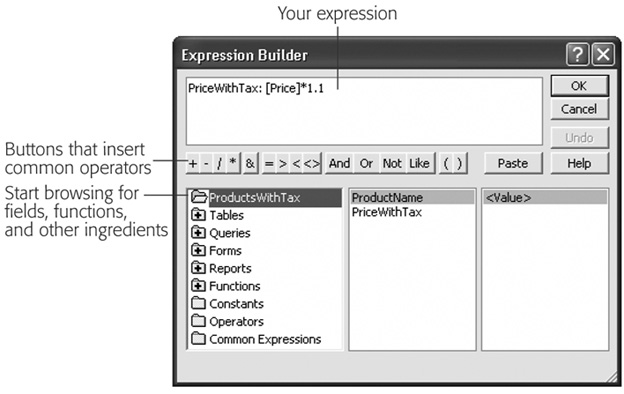
Once you choose Build, the Expression Builder appears, showing any content that’s currently in the box (Figure 7-3).
Figure 7-3. The Expression Builder consists of a text box at the top of the window, where you can edit your expression, some buttons that quickly insert common operators (like +, -, /, and *, if for some reason you can’t find them on the keyboard), and a three-paned browser at the bottom of the window that helps you find fields and functions you want to use.
Add or edit the expression.
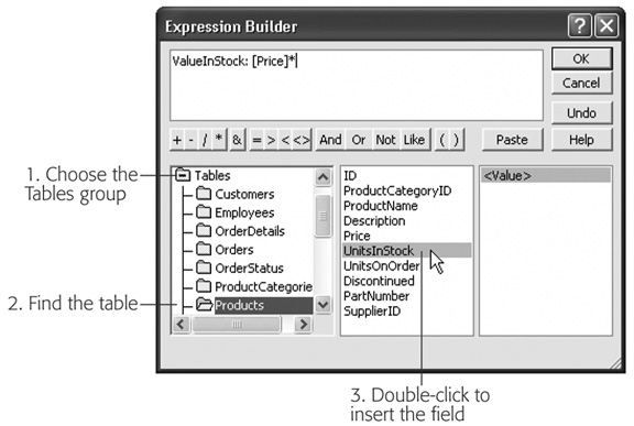
The Expression Builder includes two shortcuts that you’ll want to try. You can insert a name without typing it by hand (Figure 7-4), and you can find a function by browsing (Figure 7-5).
Figure 7-4. To pop in a new field name, double-click the Tables folder in the leftmost list. Then, click the subfolder that corresponds to the table you want to use. Finally, double-click the field name in the middle list to insert it into your expression. This technique’s recommended only for those who love to click.
Note
The Expression Builder is an all-purpose tool to create expressions for calculated fields and filter conditions. Some options make sense only in one context. The logical operators like the equals (=) symbol and the And, Or, Not, and Like operators are useful for setting criteria for filtering (Section 6.2.1.1), but don’t serve any purpose in calculated fields.
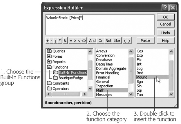
Figure 7-5. To find a function, start by double-clicking the Functions folder in the list on the left. Then, choose the Built-In Functions subfolder. (The other option shows you any custom functions that you’ve added to your database using custom VBA code.) Next, choose a function category in the middle list. The list on the right shows all the functions in that category. You can double-click the function to insert it into your expression.
Click OK.
Access copies your new expression back into the Field box or Criteria box.
Note
When you use the Expression Builder to add a function, it adds placeholders (like <number> and <precision>) where you need to supply the arguments. Replace this text with the values you want to use.
Most Access experts find that the Expression Builder is too clunky to be worth the trouble. But even though the Expression Builder may not be the most effective way to write an expression, it’s a great way to learn about new and mysterious functions, thanks to its built-in function reference. If you find a function that sounds promising but you need more information, select it in the list and then click Help. You’ll be rewarded with a brief summary that explains the purpose of the function and the arguments you need to supply, as shown in Figure 7-6.
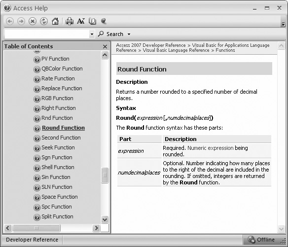
Figure 7-6. The reference for the Round( ) function spells out what it does, and explains the two parameters. One parameter—the number of decimal places—is wrapped in square brackets, which means it’s an optional value. Leave it out, and Access rounds to the nearest whole number. You’ll also notice a table of contents on the left that lets you browse to any other Access function and read its description.
Format( ) is one interesting mathematical function, which transforms numbers into text. Format( ) is interesting because the text it creates can be formatted in several different ways, which allows you to control exactly how your numbers are presented.
To understand the difference, think back to the expression you used earlier for discounting product prices:
SalePrice: [Price] * 0.95
Even if the Price field has the Currency data type, the calculated values in the SalePrice field appear as ordinary numbers (without the currency sign, thousands separator, and so on). So you see 43.2 when you might prefer $43.20.
You can remedy this problem by using the Format( ) function to apply a currency format:
SalePrice: Format([Price] / 0.95, "Currency")
Now the calculated values include the currency sign. Even better, since currencies are displayed with just two decimal places, you no longer need to clean up fractional values with the Round( ) function.
The trick to using the Format( ) function is knowing what text to supply for the second argument in order to get the result you want. Table 7-2 spells out your options.
Table 7-2. Formatting Options
|
Format |
Description |
Example |
|---|---|---|
|
Currency |
Displays a number with two decimal places, thousand separators, and the currency sign. |
$1,433.20 |
|
Fixed |
Displays a number with two decimal places. |
1433.20 |
|
Standard |
Displays a number with two decimal places and the thousands separator. |
1,433.20 |
|
Percent |
Displays a percent value (a number multiplied by 100 with a percent sign). Displays two digits to the right of the decimal place. |
143320.00% |
|
Scientific |
Displays a number in scientific notation, with two decimal places. |
1.43E+03 |
|
Displays No if the number’s 0 and Yes if the number’s anything else. You can also use the similar format types True/False and On/Off. |
Yes |
The mathematical functions in Access don’t get much respect, because people don’t need them terribly often. You’ve already seen Round( ) and Format( )—the most useful of the bunch—but there are still a few others that Access mavens turn to from time to time in calculated fields. They’re listed in Table 7-3.
Table 7-3. Functions for Numeric Data
|
Function |
Example |
Result | |
|---|---|---|---|
|
Get the square root |
Sqr(9) |
3 | |
|
Gets the absolute value (negative numbers become positive) |
Abs(-6) |
6 | |
|
Round( ) |
Rounds a number to the specified number of decimal places |
Round(8.89, 1) |
8.9 |
|
Gets the integer portion of the number, chopping off any decimal places |
Fix(8.89) |
8 | |
|
The same as Fix( ), but negative numbers are rounded down instead of up |
Int(−8.89) |
−9 | |
|
Rnd( ) |
Int ((6) * Rnd + 1) |
A random integer from 1 to 6 | |
|
Converts numeric data in a text field into a bona fide number, so that you can use it in a calculation. Stops as soon as it finds a non-numeric character, and returns 0 if it can’t find any numbers. |
Val(“315 Crossland St”) |
315 | |
|
Format( ) |
Turns a number into a formatted string, based on the options you chose |
Format(243.6, Currency) |
$243.60 |
So far, all the functions you’ve seen have worked with numeric data. However, there’s still a lot you can do with text. Overall, there are three ways you can manipulate text:
Join text. You can do things like combining several fields together into one field. This technique doesn’t require a function—instead, you can use the & operator described in Section 7.1.3.
Extract part of a text value. You may want just the first word in a title or the first 100 characters in a description.
Change the capitalization. You may want to show lowercase text in capitals, and vice versa.
Table 7-4 shows the most common functions people use with text.
Table 7-4. Functions for Text
|
Function |
Description |
Example |
Result |
|---|---|---|---|
|
Capitalizes text |
UCase(“Hi There”) |
HI THERE | |
|
Puts text in lowercase |
LCase(“Hi There”) |
hi there | |
|
Takes the number of characters you indicate from the left side |
Left(“Hi There”, 2) |
Hi | |
|
Takes the number of characters you indicate from the right side |
Right(“Hi There”, 5) |
There | |
|
Takes a portion of the string starting at the position you indicate, and with the length you indicate |
Mid(“Hi There”, 4, 2) |
Th | |
|
Removes blank spaces from either side (or use LTrim( ) and RTrim( ) to trim spaces off just the left or right side) |
Trim(“Hi There”) |
Hi There | |
|
Counts the number of characters in a text value |
Len(“Hi There”) |
8 |
Using these functions, you can create a calculated field that shows a portion of a long text value, or changes its capitalization. However, how you can use these functions in a filter expression may not be as obvious. You could create a filter condition that matches part of a text field, instead of the whole thing. Here’s an example of a filter condition that selects records that start with Choco:
Left([ProductName], 5) = "Choco"
Figure 7-7 shows how you enter this filter condition.
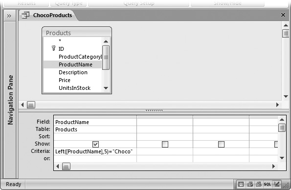
Figure 7-7. The Left( ), Right( ), and Mid( ) functions work in much the same way as the Like keyword (Section 4.3.2.3) to help you match bits and pieces of long text values.
The Len( ) function’s a bit of an oddity. It examines a text value and returns numeric information (in this case, the number of characters in the value, including all spaces, letters, numbers, and special characters). The Len( ) function isn’t too useful in a simple calculated expression, because you’ll rarely be interested in the number of letters in a text value. However, it does let you write some interesting filter conditions, including this one that grabs records with a Description of less than 15 characters (which probably could use some extra information):
Len(Description) < 15
You’ve already seen how you can use simple addition and subtraction with dates (Section 7.1.2.2). However, you can accomplish a whole lot more with some of Access’s date functions.
Without a doubt, everyone’s favorite date functions are Now( ) and Date( ), which you first saw in Chapter 4 (Section 4.3.2.3). These functions grab the current date and time, or just the current date. You can use these functions to create queries that work with the current year’s worth of orders.
Here’s a filter condition that uses Date( ) to select projects that are past due:
=<Date()
Add this to the Criteria box for the DueDate field, and you’ll see only those records that have a DueDate that falls on or before today.
Date logic becomes even more powerful when paired with the DatePart( ) function, which extracts part of the information in a date. DatePart( ) can determine the month number or year, letting you ignore other details (like the day number and the time). Using DatePart( ) and Date( ), you can easily write a filter condition like this one, which selects all the orders placed in the current month:
	DatePart("m", [DatePlaced])=DatePart("m", Date( ))
	  And DatePart("yyyy", [DatePlaced])=DatePart("yyyy", Date( ))
This rather lengthy expression’s actually a combination of two conditions joined by the And keyword. The first condition compares the month of the current date with that of the date stored in the DatePlaced field:
DatePart("m", [DatePlaced])=DatePart("m", Date())This expression establishes that they’re the same calendar month, but you also need to make sure it’s the same year:
DatePart("yyyy", [DatePlaced])=DatePart("yyyy", Date())The trick to using DatePart( ) (and several other date functions) is understanding the concept of date components. As you can see, using the text m with the DatePart( ) functions gets the month number, and using the text yyyy extracts a four-digit year. Table 7-5 shows all your options.
Table 7-5. Date Components
|
Component |
Description |
Value for February 20, 2006 1:30 PM |
|---|---|---|
|
yyyy |
Year, in four-digit format |
2006 |
|
q |
Quarter, from 1 to 4 |
1 |
|
m |
Month, from 1 to 12 |
2 |
|
y |
Day of year, from 1 to 365 (usually) |
51 |
|
d |
Day, from 1 to 31 |
20 |
|
w |
Day of week, from 1 to 7 |
2 |
|
ww |
Week of the year, from 1 to 52 |
8 |
|
h |
Hour, from 1 to 24 |
13 |
|
n |
Minute, from 1 to 60 |
30 |
|
s |
Second, from 1 to 60 |
0 |
You use the date components with several date functions, including DatePart( ), DateAdd( ), and DateDiff( ). Table 7-6 has these and more useful date-related functions.
Table 7-6. Functions for Dates
|
Function |
Example |
Result | |
|---|---|---|---|
|
Date( ) |
Gets the current date |
Date( ) |
1/20/2006 |
|
Gets the current date and time |
Now( ) |
1/20/2006 10:16:26 PM | |
|
DatePart( ) |
Extracts a part of a date (like the year, month, or day number) |
DatePart(#1/20/2006#, “d”) |
20 |
|
Converts a year, month, and day into an Access date value |
DateSerial(2006, 5, 4) |
5/4/2006 | |
|
DateAdd( ) |
Offsets a date by a given interval |
DateAdd (“yyyy”, 2, #22/11/2006#) |
22/11/2008 |
|
DateDiff( ) |
Measures an interval between two dates |
DateDiff(“w”, #10/15/2006#, #1/11/2007#) |
12 |
|
Gets the name that corresponds to a month number (from 1 to 12) |
MonthName(1) |
“January” | |
|
Gets the name that corresponds to a weekday number (from 1 to 7) |
WeekdayName(1) |
“Sunday” | |
|
Format( ) |
Converts a date into formatted text (using any of the date formats described in Section 2.3.5) |
Format (#27/04/2008#, “Long Date”) |
“April 27, 2008” |
Tip
Access has other date functions that provide part of the functionality of DatePart( ). One example’s Month( ), which extracts the month number from a date. Other duplicate functions include Year( ), Day( ), Hour( ), Minute( ), and Second( ). These functions don’t add any advantages, but you may see them used in other people’s queries to get an equivalent result.
Databases have two types of fields: required and optional. Ordinarily, fields are optional (as discussed in Section 4.1.1), which means a sloppy person can leave a lot of blank values. These blank values are called nulls, and you need to handle them carefully.
If you want to write a filter condition that catches null values, simply type this text into the criteria box:
Is Null
This condition matches any fields that are left blank. Use this on the CustomerID field in the Orders table to find any orders that aren’t linked to a customer. Or ignore unlinked records by reversing the condition, like so:
Is Not Null
Sometimes, you don’t want to specifically search for (or ignore) null values. Instead, you want to swap those values with something more meaningful to the task at hand. Fortunately, there’s an oddly named tool for just this task: the Nz( ) function.
The Nz( ) function takes two arguments. The first’s a value (usually a query field) that may contain a null value. The second parameter’s the value that you want to show in the query results if Access finds a null value. Here’s an example that uses Nz( ) to convert null values in the Quantity field to 0:
Nz([Quantity], 0)
Converting to 0 is actually the standard behavior of Nz( ), so you can leave off the second parameter if that’s what you want:
Nz([Quantity])
At this point, you may not be terribly impressed at the prospect of changing blank values in your datasheet into zeroes. But this function’s a lifesaver if you need to create calculated fields that work with values that could be null. Consider this innocent-seeming example:
OrderItemCost: [Quantity] * [Price]
This expression runs into trouble if Quantity is null. Nulls have a strange way of spreading, somewhat like an invasive fungus. If you have a null anywhere in a calculation, the result of that calculation is automatically null. In this example, that means the OrderItemCost for that record becomes null. Even worse, if the OrderItemCost enters into another calculation or a subtotal, that too becomes null. Before you know it, your valuable query data turns into a ream of empty cells.
To correct this problem, use the Nz( ) function to clean up any potential nulls in optional fields:
OrderItemCost: Nz([Quantity]) * Nz([Price])
Finally, you can use Nz( ) to supply a different value altogether. In a text field, you may choose to enter something more descriptive. Here’s an example that displays the text [Not Entered] next to any record that doesn’t include name information:
Name: Nz ([FirstName] & " " & [LastName], "[Not Entered]")
All the queries you’ve used so far work with individual records. If you select 143 records from an Orders table, you see 143 records in your results. You can also group your records to arrive at totals and subtotals. That way, you can review large quantities of information much more easily, and make grand, sweeping conclusions.
Some examples of useful summarizing queries include:
Counting all the students in each class
Counting the number of orders placed by each customer
Totaling the amount of money spent on a single product
Totaling the amount of money a customer owes or has paid
Calculating the average order placed by each customer
Finding the highest or lowest priced order that a customer has placed
These operations—counting, summing, averaging, and finding the maximum and minimum value—are the basic options in a totals query. A totals query’s a different sort of query that’s designed to chew through a large number of records and spit out neat totals.
To create a totals query, follow these steps:
Create a new query by choosing Create → Other → Query Design.
Add the tables you want to use from the Show Table dialog box, and then click Close.
The following example uses the Products table from the Boutique Fudge database.
Add the fields you want to use.
This example uses the Price field, but with a twist: the Price field is added three separate times. That’s because the query will show the result of three different calculations.
Choose Query Tools | Design → Show/Hide → Totals.
Access adds a Total box for each field, just under the Table box.
For each field, choose an option from the Total box. This option determines whether the field is used in a calculation or used for grouping.
A totals query is slightly different from a garden-variety query. Every field must fall into one of these categories:
It’s used in a summary calculation (like averaging, counting, and so on). You pick the type of calculation you want to perform using the Total box. Table 7-7 describes all the options in the Total box.
It’s used for grouping. Ordinarily, a totals query lumps everything together in one grand total. But you can subdivide the results into smaller subtotals, as described in the next section.
It’s used for filtering. In this case, in the Total box, you need to choose WHERE. (Database nerds may remember that Where is the keyword used to define criteria in SQL, as described in Section 6.2.3.1.) You also need to clear the checkmark in the Show box, because Access doesn’t have a way to show individual values in a totals summary.
Note
If you try to add a field to a totals query that isn’t used for a calculation, isn’t used for grouping, and isn’t hidden, you’ll receive an error when you try to run the query.
In this example (Figure 7-8), the Price field uses three different summarizing options: Max, Min, and Avg.
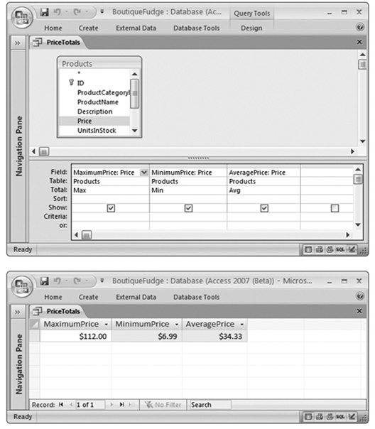
Figure 7-8. Top: This totals query includes the same field—Price—thrice, and uses three difficult calculations. Notice that each field uses an expression that provides a more descriptive name (Section 7.1.2). Bottom: The results show a single record with the maximum price, minimum price, and average price of the products sold by Boutique Fudge.
Note
Table 7-7 leaves out two options that are tailor-made for statisticians—StDev and Var—which calculate the standard deviation and variance of a set of numbers.
Table 7-7. Options for Summarizing Data
|
Choice in the Total Box |
Description |
|---|---|
|
Subgroups records based on the values in this field | |
|
Sum |
Adds together the values in this field |
|
Averages the values in this field | |
|
Retains the smallest value in this field | |
|
Retains the largest value in this field | |
|
Counts the number of records (no matter which field you use) | |
|
Retains the first value in this field | |
|
Retains the last value in this field |
You can use all the same query-writing skills you picked up earlier in this chapter when designing a totals query. If you want to summarize only the products in a specific category, you can use a filter expression like this in the CategoryID field:
=3
This expression matches records that have a CategoryID of 3 (which means they’re in the Candies category).
Note
If you want to perform a filter on a field that you aren’t using for a calculation or grouping, make sure that in the Total box, you choose Where, and in the Show box, you clear the checkmark.
The simplest possible totals query adds all the records you select into a single row of results, as shown in Figure 7-8. A more advanced totals query uses grouping to calculate subtotals.
The trick to using grouping properly is remembering that the field you use should have many duplicate values. For example, it’s a good idea to group customers based on the state in which they live. Because a given state has many customers, you’ll end up with meaningful subtotals. However, it’s a bad idea to group them based on their Social Security numbers, because you’ll end up with just as many groups as you have customers. Figure 7-9 shows an example of totals query that uses grouping.
You can use multiple levels of grouping in a totals query by adding more than one field with the Total box set to Group By. However, the results might not be exactly what you expect. Suppose you group a long list of sales records by product and by customer. You’ll end up with a separate group for every customer-and-product combination. Here’s part of the results for a query like this that groups records from the OrderDetails table in the Boutique Fudge database and then sorts them by CustomerID:
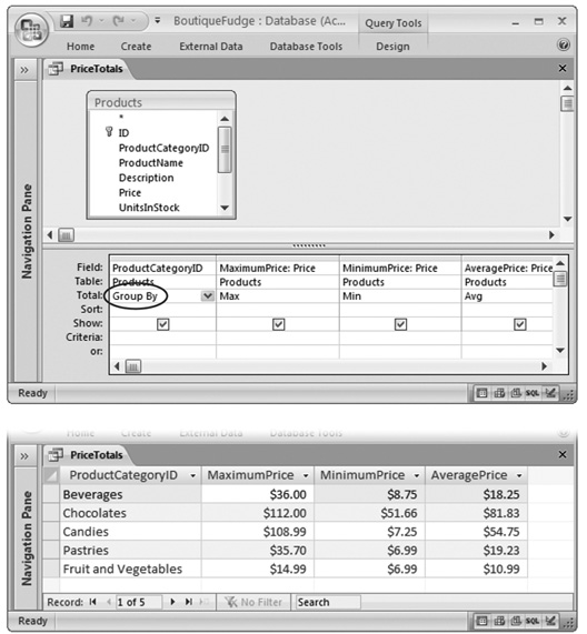
Figure 7-9. Top: Here, products are grouped by product category. Bottom: The result: a separate row with the totals for each product category.
This table tells you that customer #10 has spent a total of $432.12 dollars on product #108 across all orders. Customer #10 also spent a total of $16.79 on product #134, $53.30 on product #210, and so on. (You could take the same information and sort it by ProductID to look at the total sales of each product to different customers. You still get the same information, but you can analyze it in a different way.)
This is the result you want—sort of. It lacks nice subtotals. It would be nice to know how much customer #10 spent on each type of product, and how much customer #10 spent in total. But thanks to the rigid tabular structure of the totals query, this result just isn’t possible.
If you want to look at this subgrouped information with subtotals, you have two choices. You can use a crosstab query or a pivot-table query—two advanced summary options that are described in Chapter 9. Or, if you’re really interested in printing out your information, you can generate a report that includes multiple levels of grouping and subtotals, as described in Part Three.
Summary queries are insanely useful when you combine them with table joins (Section 6.3) to get related information out of more than one table. In the Boutique Fudge database, the OrderDetails table stores the individual items in each order. You can group this information (as shown in the previous section) to find top-selling products or customers. However, you see only the customer and product ID values, which isn’t very helpful.
Note
If you have a lookup defined on the ProductID field and CustomerID field, you will see the descriptive information from the lookup (like the product name or customer name). This information helps a bit, but you may still want to pull extra information—like the customer’s address, the product description, and so on—out of the linked table.
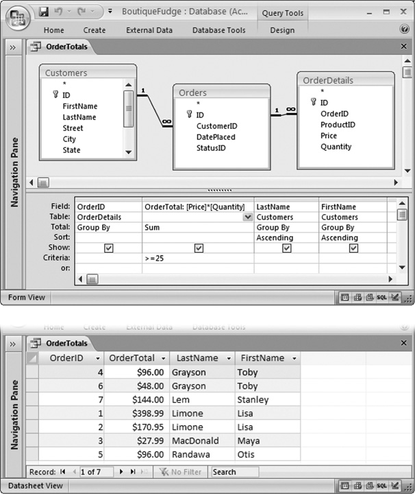
If you throw a join or two into the mix, you can pull in related information from linked tables (like Customers, Products, and Orders) and add it to your results. Figure 7-10 shows an example that groups the OrderDetails table by OrderID to find the total cost of each order. It then sorts the results by CustomerID.
You already know enough to build the query shown in Figure 7-10. Here’s what you need to do:
Create a new query by choosing Create → Other → Query Design.
Add the tables you want to use from the Show Table dialog box, and then click Close.
The example in Figure 7-10 uses the Customers, Orders, and OrderDetails tables. As you add these tables, Access fills in the join lines in between, based on the relationships defined in your database.
Choose Query Tools | Design → Show/Hide → Totals.
This adds the Total box for each field.
Figure 7-10. Top: This totals query gets more advanced by drawing from three related tables—Customers, Orders, and OrderDetails—to show a list of order totals, organized by customer. The query ignores orders less than $25. You could also add a filter expression on the DatePlaced field to find out how much customers spent so far this year, how much they spent last year, how much they spent last week, and so on. Bottom: The results are grouped by OrderID and sorted by LastName and FirstName, which preserves a good level of detail.
Add the fields you want to use, and then, in the Total box, choose the appropriate grouping or summarizing option for each one.
You can choose your fields from any of the linked tables. This example uses several fields:
OrderID. This field’s used to group the results. In other words, you want to total all the records in the OrderDetails table that have the same OrderID. To make this work, in the Total box, choose Group By. (Incidentally, it makes no difference whether you choose the OrderID field in the OrderDetails table or the ID field in the Orders table—they’re both linked.)
OrderTotal. This field’s a calculated field that uses the expression [Price]*[Quantity] to multiply together two fields from the OrderDetails table. The result’s the total for that individual line of the order. Access adds up all these line totals to create the grand order total, so set the Total box to Sum. In addition, the OrderTotal field includes the filter expression >=25, which hides any orders that have a combined value of less than $25.
LastName and FirstName. These fields identify the customer who made the order. However, there’s a trick here. In order to show any field in a totals query, you need to perform a calculation on it (as with OrderTotal) or use it for grouping (as with OrderID). That means you must set the Total box to Group By for both LastName and FirstName. However, this setting doesn’t actually have an effect, because every order’s always placed by a single customer. (In other words, you’ll never find a bunch of records in the OrderDetails table that are for the same order but for different customers. It just isn’t possible.) The end result is that Access doesn’t perform any grouping on the LastName and FirstName fields. Instead, they’re simply displayed next to every order.
Note
This grouping trick’s a little weird, but it’s a common technique in totals queries. Just remember, Access creates the smallest groups it can. If you want to group by customers only (so you can see how much everyone spends), you simply need to remove the OrderID grouping and group on CustomerID instead. Or, if you want to total all the sales of a particular product, remove all the customer information, group on ProductID, and then add any extra fields you want to see from the Products table (like Product-Name and Description).
You can now run your query.
Query parameters are the Access database’s secret weapon. Query parameters let you create supremely flexible queries by intentionally leaving out one (or more) pieces of information. Every time you run the query, Access prompts you to supply the missing values. These missing values are the query parameters.
Usually, you use query parameters in filter conditions. Suppose you want to view the customers who live in a specific state. You could create a whole range of different queries, like NewYorkCustomers, CaliforniaCustomers, OhioCustomers, and so on. If you’re really interested in only a few states, this approach makes sense. But if you want to work with each and every one, it’s better to create a single query that uses a parameter for the state information. When you run the query, you fill in the state you want to use at that particular moment.
To create a query that uses parameters, follow these steps:
Create a new query by choosing Create → Other → Query Design.
From the Show Table dialog box, add the tables you want to use, and then click Close.
This example uses the Customers table.
Choose Query Tools | Design → Show/Hide → Parameters.
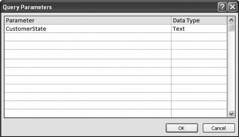
Choose a name and data type for your parameter (Figure 7-11).
You can use any name you want (but don’t choose a name that’s already in use for a field in your query). The data type should match the field on which you’re using the parameter. You set the data type by choosing one of the options in the drop-down list. Common choices are Text, Integer, Currency, and Date/Time.
Now you can use the parameter by name, in the same way that you’d refer to a field in your query. For example, you can add the following filter condition to the State field:
[CustomerState]
Make sure you keep the square brackets so Access knows you’re not trying to enter a piece of text.
When you run this query, Access pops open the Enter Parameter Value dialog box, asking for a value (Figure 7-12). Enter the state you’re interested in, and then click OK. Access uses your value for the filter on the State field.
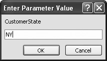
Figure 7-12. Every time you run this query, you can home in on a different state. Here, you’re about to see customers in New York.
Tip
Even though you can, it’s best not to use more than one query parameter in the same query. When you run a query, Access shows a separate Enter Parameter Value dialog box for each value. If you have a handful of parameters, then you need to click your way through an annoying number of windows.
There’s no shortage of practical ways to use query parameters. You could adapt a yearly sales query to use whatever year you choose. You could work similar magic to create a single query to show sales from any month.
However, you shouldn’t use query parameters to help you out with day-to-day data-entry tasks (like updating a single customer record). Forms, which you’ll begin building in Part Four, give you a more powerful way to browse and edit information.