CHAPTER 10
Low Bit-Rate Coding: Theory and Evaluation

In a world of limitless storage capacity and infinite bandwidth, digital signals could be coded without regard to file size, or the number of bits needed for transmission. While such a world may some day be approximated, today there is a cost for storage and bandwidth. Thus, for many applications, it is either advantageous or mandated that audio signals be coded as bit-efficient as possible. Accomplishing this task while preserving audio fidelity is the domain of low bit-rate coding. Two approaches are available. One approach uses perceptual coding to reduce file size while avoiding significant audible loss and degradation. The art and science of lossy coding combines the perceptual qualities of the human ear with the engineering realities of signal processing. A second approach uses lossless coding in which file size is compressed, but upon playback the original uncompressed file is restored. Because the restored file is bit-for-bit identical to the original, there is no change in audio fidelity. However, lossless compression cannot achieve the same amount of data reduction as lossy methods. Both approaches can offer distinct advantages over traditional PCM coding.

This chapter examines the theory of perceptual (lossy) coding, as well as the theory of lossless data compression. In addition, ways to evaluate the audible quality of perceptual codecs are presented. Chapter 11 more fully explores the details of particular codecs, both lossy and lossless. The more specialized nature of speech coding is described in Chap. 12.

Perceptual Coding

Edison cylinders, like all analog formats, store acoustical waveforms with a mimicking pattern—an analog—of the original sonic waveform. Some digital media, such as the Compact Disc, do essentially the same thing, but replace the continuous mechanical pattern with a discrete series of numbers that represents the waveform’s sampled amplitude. In both cases, the goal is to reconstruct a waveform that is physically identical to the original within the audio band. With perceptual (lossy) coding, physical identity is waived in favor of perceptual identity. Using a psychoacoustic model of the human auditory system, the codec (encoder-decoder) identifies imperceptible signal content (to remove irrelevancy) as bits are allocated. The signal is then coded efficiently (to avoid redundancy) in the final bitstream. These steps reduce the quantity of data needed to represent an audio signal but also increase quantization noise. However, much of the quantization noise can be shaped and hidden below signal-dependent thresholds of hearing. The method of lossy coding asks the conceptual question—how much noise can be introduced to the signal without becoming audible?

Through psychoacoustics, we can understand how the ear perceives auditory information. A perceptual coding system strives to deliver all of perceived information, but no more. A perceptual coding system recognizes that sounds that are reproduced have the human ear as the intended receiver. A perceptual codec thus strives to match the sound to the receiver. Logically, the first step in designing such a codec is to understand how the human ear works.

Psychoacoustics

When you hear a plucked string, can you distinguish the fifth harmonic from the fundamental? How about the seventh harmonic? Can you tell the difference between a 1000-Hz and a 1002-Hz tone? You are probably adept at detecting this 0.2% difference. Have you ever heard “low pitch” in which complex tones seem to have a slightly lower subjective pitch than pure tones of the same frequency? All this and more is the realm of psychoacoustics, the study of human auditory perception, ranging from the biological design of the ear to the psychological interpretation of aural information. Sound is only an academic concept without our perception of it. Psychoacoustics explains the subjective response to everything we hear. It is the ultimate arbitrator in acoustic concerns because it is only our response to sound that fundamentally matters. Psychoacoustics seeks to reconcile acoustic stimuli and all the scientific, objective, and physical properties that surround them, with the physiological and psychological responses evoked by them.

The ear and its associated nervous system is an enormously complex, interactive system with incredible powers of perception. At the same time, even given its complexity, it has real limitations. The ear is astonishingly acute in its ability to detect a nuance or defect in a signal, but it is also surprisingly casual with some aspects of the signal. Thus the accuracy of many aspects of a coded signal can be very low, but the allowed degree of diminished accuracy is very frequency- and time-dependent.

Arguably, our hearing is our most highly developed sense; in contrast, for example, the eye can only perceive frequencies over one octave. As with every sense, the ear is useful only when coupled to the interpretative powers of the brain. Those mental judgments form the basis for everything we experience from sound and music. The left and right ears do not differ physiologically in their capacity for detecting sound, but their respective right- and left-brain halves do. The two halves loosely divide the brain’s functions. There is some overlap, but the primary connections from the ears to the brain halves are crossed; the right ear is wired to the left-brain half and the left ear to the right-brain half. The left cerebral hemisphere processes most speech (verbal) information. Thus, theoretically the right ear is perceptually superior for spoken words. On the other hand, it is mainly the right temporal lobe that processes melodic (nonverbal) information. Therefore, we may be better at perceiving melodies heard by the left ear.

Engineers are familiar with the physical measurements of an audio event, but psychoacoustics must also consider the perceptual measurements. Intensity is an objective physical measurement of magnitude. Loudness, first introduced by physicist Georg Heinrich Barkhausen, is the perceptual description of magnitude that depends on both intensity and frequency. Loudness cannot be empirically measured and instead is determined by listeners’ judgments. Loudness can be expressed in loudness levels called phons. A phon is the intensity of an equally loud 1-kHz tone, expressed in dB SPL. Loudness can also be expressed in sones, which describe loudness ratios. One sone corresponds to the loudness of a 40 dB SPL sine tone at 1 kHz. A loudness of 2 sones corresponds to 50 dB SPL. Similarly, any doubling of loudness in sones results in a 10-dB increase in SPL. For example, a loudness ratio of 64 sones corresponds to 100 dB SPL.

The ear can accommodate a very wide dynamic range. The threshold of feeling at 120 dB SPL has a sound intensity that is 1,000,000,000,000 times greater than that of the threshold of hearing at 0 dB SPL. The ear’s sensitivity is remarkable; at 3 kHz, a threshold sound displaces the eardrum by a distance that is about one-tenth the diameter of a hydrogen atom. For convenience of expression, it is clear why the logarithmic decibel is used when dealing with the ear’s extreme dynamic range. The ear is also fast; within 500 ms of hearing a maximum-loudness sound, the ear is sensitive to a threshold sound. Thus, whereas the eye only slowly adjusts its gain for different lighting levels and operates over a limited range at any time, the ear operates almost instantaneously over its full range. Moreover, whereas the eye can perceive an interruption to light that is 1/60 second, the ear may detect an interruption of 1/500 second.

Although the ear’s dynamic range is vast, its sensitivity is frequency-dependent. Maximum sensitivity occurs at 1 kHz to 5 kHz, with relative insensitivity at low and high frequencies. This is because of the pressure transfer function that is an intrinsic part of the design of the middle ear. Through testing, equal-loudness contours such as the Robinson–Dadson curves have been derived, as shown in Fig. 10.1. Each contour describes a range of frequencies that are perceived to be equally loud. The lowest contour describes the minimum audible field, the minimum sound pressure level across the audible frequency band that a person with normal hearing can perceive. For example, a barely audible 30-Hz tone would be 60 dB louder than a barely audible 4-kHz tone. The response varies with respect to level; the louder the sounds, the flatter our loudness response. The contours are rated in phons, measuring the SPL of a contour at 1 kHz.

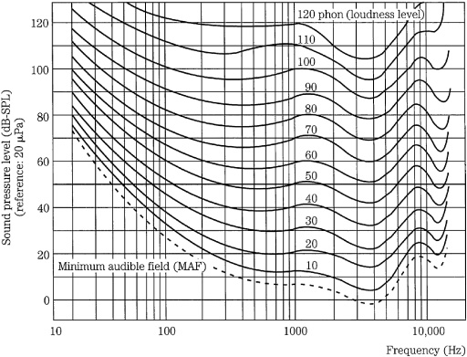
FIGURE 10.1 The Robinson–Dadson equal-loudness contours show that the ear is nonlinear with respect to frequency and level. These contours are based on psychoacoustic studies, using sine tones. (Robinson and Dadson, 1956)

Frequency is a literal measurement. Pitch is a subjective, perceptual measure. Pitch is a complex characteristic based on frequency, as well as other physical quantities such as waveform and intensity. For example, if a 200-Hz sine wave is sounded at a soft then louder level, most listeners will agree that the louder sound has a lower pitch. In fact, a 10% increase in frequency might be necessary to maintain a listener’s subjective evaluation of a constant pitch at low frequencies. On the other hand, in the ear’s most sensitive region, 1 kHz to 5 kHz, there is almost no change in pitch with loudness. Also, with musical tones, the effect is much less. Looked at in another way, pitch, quite unlike frequency, is purely a musical characteristic that places sounds on a musical scale.

The ear’s response to frequency is logarithmic; this can be demonstrated through its perception of musical intervals. For example, the interval between 100 Hz and 200 Hz is perceived as an octave, as is the interval between 1000 Hz and 2000 Hz. In linear terms, the second octave is much larger, yet the ear hears it as the same interval. For this reason, musical notation uses a logarithmic measuring scale. Each four and one-half spaces or lines on the musical staff represent an octave, which might be only a few tens of Hertz apart, or a few thousands, depending on the clef and ledger lines used.

Beat frequencies occur when two nearly equal frequencies are sounded together. The beat frequency is not present in the audio signal, but is an artifact of the ear’s limited frequency resolution. When the difference in frequency between tones is itself an audible frequency, a difference tone can be heard. The effect is especially audible when the frequencies are high, the tones fairly loud, and separated by not much more than a fifth. Although debatable, some listeners claim to hear sum tones. An inter-tone can also occur, especially below 200 Hz where the ear’s ability to discriminate between simultaneous tones diminishes. For example, simultaneous tones of 65 Hz and 98 Hz will be heard not as a perfect fifth, but as an 82-Hz tone. On the other hand, when tones below 500 Hz are heard one after the other, the ear can differentiate between pitches only 2 Hz apart.

The ear-brain is adept at determining the spatial location of sound sources, using a variety of techniques. When sound originates from the side, the ear-brain uses cues such as intensity differences, waveform complexity, and time delays to determine the direction of origin. When equal sound is produced from two loudspeakers, instead of localizing sound from the left and right sources, the ear-brain interprets sound coming from a space between the sources. Because each ear receives the same information, the sound is stubbornly decoded as coming from straight ahead. Similarly, stereo is nothing more than two different monaural channels. The rest is simply illusion.

There is probably no limit to the complexity of psychoacoustics. For example, consider the musical tones in Fig. 10.2A. A scale is played through headphones to the right and left ears. Most listeners hear the pattern in Fig. 10.2B, where the sequence of pitches is correct, but heard as two different melodies in contrary motion. The high tones appear to come from the right ear, and the lower tones from the left. When the headphones are reversed, the headphone formerly playing low tones now appears to play high tones, and vice versa. Other listeners might hear low tones to the right and high tones to the left, no matter which way the headphones are placed. Curiously, right-handed listeners tend to hear high tones on the right and lows on the left; not so with lefties. Still other listeners might perceive only high tones and little or nothing of the low tones. In this case, most right-handed listeners perceive all the tones, but only half of the lefties do so.

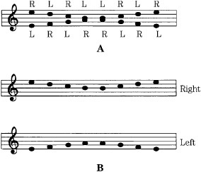
FIGURE 10.2 When a sequence of two-channel tones is presented to a listener, perception might depend on handedness. A. Tones presented to listener. B. Illusion most commonly perceived. (Deutsch, 1983)

The ear perceives only a portion of the information in an audio signal; that perceived portion is the perceptual entropy—estimated to be as low as 1.5 bits/sample. Small entropy signals can be efficiently reduced; large entropy signals cannot. For this reason, a codec might output a variable bit rate that is low when information is poor, and high when information is rich. The output is variable because although the sampling rate of the signal is constant, the entropy in its waveform is not. Using psychoacoustics, irrelevant portions of a signal can be removed; this is known as data reduction. The original signal cannot be reconstructed exactly. A data reduction system reduces entropy; by modeling the perceptual entropy, only irrelevant information is removed, hence the reduction can be inaudible. A perceptual music codec does not attempt to model the music source (a difficult or impossible task for music coding); instead, the music signal is tailored according to the receiver, the human ear, using a psychoacoustic model to identify irrelevant and redundant content in the audio signal. In contrast, some speech codecs use a model of the source, the vocal tract, to estimate speech characteristics, as described in Chap. 12.

Traditionally, audio system designers have used objective parameters as their design goals—flat frequency response, minimal measured noise, and so on. Designers of perceptual codecs recognize that the final receiver is the human auditory system. Following the lead of psychoacoustics, they use the ear’s own performance as the design criterion. After all, any musical experience—whether created, conveyed, and reproduced via analog or digital means—is purely subjective.

Physiology of the Human Ear and Critical Bands

The ear uses a complex combination of mechanical and neurological processes to accomplish its task. In particular, the ear performs the transformation from acoustical energy to mechanical energy and ultimately to the electrical impulses sent to the brain, where information contained in sound is perceived. A simplified look at the human ear’s physiological design is shown in Fig. 10.3. The outer ear collects sound, and its intricate folds help us to assess directionality. The ear canal resonates at around 3 kHz to 4 kHz, providing extra sensitivity in the frequency range that is critical for speech intelligibility. The eardrum transduces acoustical energy into mechanical energy; it reaches maximum excursion at about 120-dB SPL, above which it begins to distort the waveform. The three bones in the middle ear, colloquially known as the hammer, anvil, and stirrup (the three smallest bones in the body) provide impedance matching to efficiently convey sounds in air to the fluid-filled inner ear. The vestibular canals do not affect hearing, but instead are part of a motion detection system providing a sense of balance. The coiled basilar membrane detects the amplitude and frequency of sound; those vibrations are converted to electrical impulses and sent to the brain as neural information along a bundle of nerve fibers. The brain decodes the period of the stimulus and point of maximum stimulation along the basilar membrane to determine frequency; activity in local regions surrounding the stimulus is ignored.

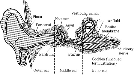
FIGURE 10.3 A simplified look at the physiology of the human ear. The coiled cochlea and basilar membrane are straightened for clarity of illustration.

Examination of the basilar membrane shows that the ear contains roughly 30,000 hair cells arranged in multiple rows along the basilar membrane, roughly 32 mm long; this is the Organ of Corti. The cells detect local vibrations of the basilar membrane and convey audio information to the brain via electrical impulses. The decomposition of complex sounds into constituent components is analogous to Fourier analysis and is known as tonotopicity. Frequency discrimination dictates that at low frequencies, tones a few Hertz apart can be distinguished; however, at high frequencies, tones must differ by hundreds of Hertz. In any case, hair cells respond to the strongest stimulation in their local region; this region is called a critical band, a concept introduced by Harvey Fletcher in 1940.

Fletcher’s experiments showed that, for example, when noise masks a pure tone, only frequency components of the noise that are near the frequency of the tone are relevant in masking the tone. Energy outside the band is inconsequential. This frequency range of relevancy is the critical band. Critical bands are much narrower at low frequencies than at high frequencies; three-fourths of the critical bands are below 5 kHz; in terms of masking, the ear receives more information from low frequencies and less from high frequencies. When critical bandwidths are plotted with respect to critical-band center frequency, critical bandwidths are approximately constant from 0 Hz to 500 Hz, and then approximately proportional to frequency from about 500 Hz upward, as shown in Fig. 10.4. In other words, at higher frequencies, critical bandwidth increases approximately linearly as the center frequency increases logarithmically.

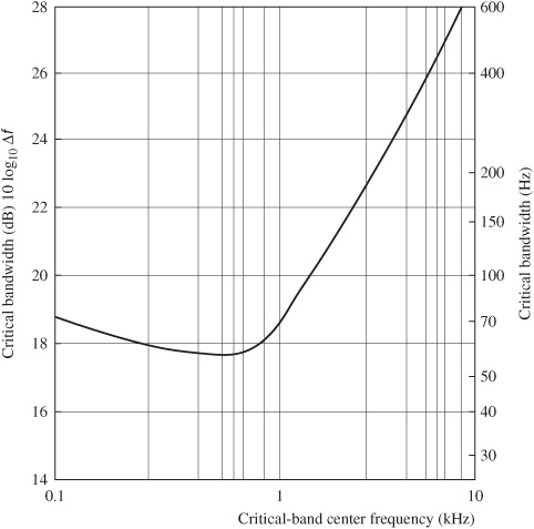
FIGURE 10.4 A plot showing critical bandwidths for monaural listening. (Goldberg and Riek, 2000)

Critical bands are approximately 100 Hz wide for frequencies from 20 Hz to 500 Hz and approximately 1.5 octaves in width for frequencies from 1 kHz to 7 kHz. Alternatively, bands can be assumed to be 1.3 octaves wide for frequencies from 300 Hz to 20 kHz; an error of less than 1.5 dB will occur. Other research shows that critical bandwidth can be approximated with the equation:

Critical bandwidth = 25 + 75[1 + 1.4(f /1000)²]^0.69 Hz

where f = center frequency in Hz.

The ear was modeled by Eberhard Zwicker with 24 arbitrary critical bands for frequencies below 15 kHz; a 25th band occupies the region from 15 kHz to 20 kHz. An example of critical band placement and width is listed in Table 10.1. Physiologically, each critical band occupies a length of about 1.3 mm, with 1300 primary hair cells. The critical band for a 1-kHz sine tone is about 160 Hz in width. Thus, a noise or error signal that is 160 Hz wide and centered at 1 kHz is audible only if it is greater than the same level of a 1-kHz sine tone. Critical bands describe a filtering process in the ear; they describe a system that is analogous to a spectrum analyzer showing the response patterns of overlapping bandpass filters with variable center frequencies. Importantly, critical bands are not fixed; they are continuously variable in frequency, and any audible tone will create a critical band centered on it. The critical band concept is an empirical phenomenon. Looked at in another way, a critical band is the bandwidth at which subjective responses change. For example, if a band of noise is played at a constant sound-pressure level, its loudness will be constant as its bandwidth is increased. But as its bandwidth exceeds that of a critical band, the loudness increases.

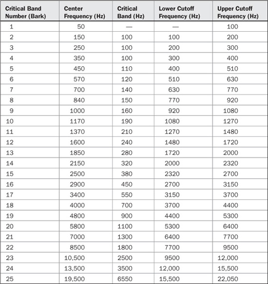
TABLE 10.1 An example of critical bands in the human hearing range showing an increase in bandwidth with absolute frequency. A critical band will arise at an audible sound at any frequency. (after Tobias, 1970)

Most perceptual codecs rely on amplitude masking within critical bands to reduce quantized word lengths. Masking is the essential trick used to perceptually hide coding noise. Indeed, in the same way that Nyquist is honored for his famous sampling frequency relationship, modern perceptual codecs could be called “Fletcher codecs.”

Interestingly, critical bands have also been used to explain consonance and dissonance. Tone intervals with a frequency difference greater than a critical band are generally more consonant; intervals less than a critical band tend to be dissonant with intervals of about 0.2 critical bandwidth being most dissonant. Dissonance tends to increase at low frequencies; for example, musicians tend to avoid thirds at low frequencies. Psychoacousticians also note that critical bands play a role in the perception of pitch, loudness, phase, speech intelligibility, and other perceptual matters.

The Bark (named after Barkhausen) is a unit of perceptual frequency. Specifically, a Bark measures the critical-band rate. A critical band has a width of 1 Bark; 1/100 of a Bark equals 1 mel. The Bark scale relates absolute frequency (in Hertz) to perceptually measured frequencies such as pitch or critical bands (in Bark). Conversion from frequency to Bark can be accomplished with:

z(f) = 13arctan(0.00076f) + 3.5arctan[(f/7500)²] Bark

where f = frequency in Hz.

Using a Bark scale, the physical spectrum can be converted to a psychological spectrum along the basilar membrane. In this way, a pure tone (a single spectral line) can be represented as a psychological-masking curve. When critical bands are plotted using a Bark scale, they are relatively consistent with frequency, verifying that the Bark is a “natural” unit that presents the ear’s response more accurately than linear or logarithmic plots. However, the shape of masking curves still varies with respect to level, showing more asymmetric slopes at louder levels.

Some researchers prefer to characterize auditory filter shapes in terms of an equivalent rectangular bandwidth (ERB) scale. The ERB represents the bandwidth of a rectangular function that conveys the same power as a critical band. The ERB scale portrays auditory filters somewhat differently than the critical bandwidth representation. For example, ERB argues that auditory filter bandwidths do not remain constant below 500 Hz, but instead decrease at lower frequencies; this would require greater low-frequency resolution in a codec. In one experiment, the ERB was modeled as:

ERB = 24.7[4.37(f/1000)+ 1] Hz

where f = center frequency in Hz.

The pitch place theory further explains the action of the basilar membrane in terms of a frequency-to-place transformation. Carried by the surrounding fluid, a sound wave travels the length of the membrane and creates peak vibration at particular places along the length of the membrane. The collective stimulation of the membrane is analyzed by the brain, and frequency content is perceived. High frequencies cause peak response at the membrane near the middle ear, while low frequencies cause peak response at the far end. For example, a 500-Hz tone would create a peak response at about three-fourths of the distance along the membrane. Because hair cells tend to vibrate at the frequency of the strongest stimulation, they will convey that frequency in a critical band, ignoring lesser stimulation. This excitation curve is described by the cochlear spreading function, an asymmetrical contour. This explains, for example, why broadband measurements cannot describe threshold phenomena, which are based on local frequency conditions. There are about 620 degrees of differentiable frequencies equally distributed along the basilar membrane; thus, a resolution of 1.25 Bark is reasonable. Summarizing, critical bands are important in perceptual coding because they show that the ear discriminates between energy in the band, and energy outside the band. In particular, this promotes masking.

Threshold of Hearing and Masking

Two fundamental phenomena that govern human hearing are the minimum-hearing threshold and amplitude masking, as shown in Fig. 10.5. The threshold of hearing curve describes the minimum level (0 sone) at which the ear can detect a tone at a given frequency. The threshold is referenced to 0 dB at 1 kHz. The ear is most sensitive in the 1-kHz to 5-kHz range, where we can hear signals several decibels below the 0-dB reference. Generally, two tones of equal power and different frequency will not sound equally loud. Similarly, the audibility of noise and distortion varies according to frequency. Sensitivity decreases at high and low frequencies. For example, a 20-Hz tone would have to be approximately 70 dB louder than a 1-kHz tone to be barely audible. A perceptual codec compares the input signal to the minimum threshold, and discards signals that fall below the threshold; the signals are irrelevant because the ear cannot hear them. Likewise, a codec can safely place quantization noise under the threshold because it will not be heard. The absolute threshold of hearing is determined by human testing, and describes the energy in a pure tone needed for audibility in a noiseless environment. The contour can be approximated by the equation:

T(f) = 3.64(f/1000)^−0.8 − 6.5e^{−0.6[(f/1000)−3.3]2} + 10⁻³(f/1000)⁴ dB SPL

where f = frequency in Hz.

This threshold is absolute, but a music recording can be played at loud or soft levels—a variable not known at the time of encoding. To account for this variation, many codecs conservatively equate the decoder’s lowest output level to a 0-dB level or alternatively to the −4-dB minimum point of the threshold curve, near 4 kHz. In other words, the ideal (lowest) quantization error level is calibrated to the lowest audible level. Conversely, this corresponds to a maximum value of about 96 dB SPL for a 16-bit PCM signal. Some standards refer to the curve as the threshold of quiet.

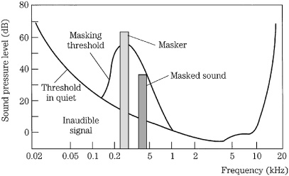
FIGURE 10.5 The threshold of hearing describes the softest sounds audible across the human hearing range. A masker tone or noise will raise the threshold of hearing in a local region, creating a masking curve. Masked tones or noise, perhaps otherwise audible, that fall below the masking curve during that time will not be audible.

When tones are sounded simultaneously, amplitude masking occurs in which louder tones can completely obscure softer tones. For example, it is difficult to carry on a conversation in a nightclub; the loud music masks the sound of speech. More analytically, for example, a loud 800-Hz tone can mask softer tones of 700 Hz and 900 Hz. Amplitude masking shifts the threshold curve upward in a frequency region surrounding the tone. The masking threshold describes the level where a tone is barely audible. In other words, the physical presence of sound certainly does not ensure audibility and conversely can ensure inaudibility of other sound. The strong sound is called the masker and the softer sound is called the maskee. Masking theory argues that the softer tone is just detectable when its energy equals the energy of the part of the louder masking signal in the critical band; this is a linear relationship with respect to amplitude. Generally, depending on relative amplitude, soft (but otherwise audible) audio tones are masked by louder tones at a similar frequency (within 100 Hz at low frequencies). A perceptual codec can take advantage of masking; the music signal to be coded can mask a relatively high level of quantization noise, provided that the noise falls within the same critical band as the masking music signal and occurs at the same time.

The mechanics of the basilar membrane explain the phenomenon of amplitude masking. A loud response at one place on the membrane will mask softer responses in the critical band around it. Unless the activity from another tone rises above the masking threshold, it will be swamped by the masker. Figure 10.6A shows four masking curves (tones masked by narrow-band noise) at 60 dB SPL, on a logarithmic scale in Hertz. Figure 10.6B shows seven masking curves on a Bark scale; using this natural scale, the consistency of the critical-band rate is apparent. Moreover, this plot illustrates the position of critical bands along the basilar membrane.

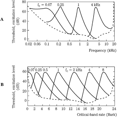
FIGURE 10.6 Masking curves describe the threshold where a tone or noise is just audible in the presence of a masker. Threshold width varies with frequency when plotted logarithmically. When plotted on a Bark scale, the widths and slopes are similar, reflecting response along the basilar membrane. A. Masking thresholds plotted with logarithmic frequency. B. Masking thresholds plotted with critical-band rate. (Zwicker and Zwicker, 1991)

Masking thresholds are sometimes expressed as an excitation level; this is obtained by adding a 2-dB to 6-dB masking index to the sound pressure level of the just-audible tone. Low frequencies can interfere with the perception of higher frequencies. Masking can overlap adjacent critical bands when a signal is loud, or contains harmonics; for example, a complex 1-kHz signal can mask a simple 2-kHz signal. Low amplitude signals provide little masking. Narrow-band tones such as sine tones also provide relatively little masking. Likewise, louder, more complex tones provide greater masking with masking curves that are broadened, and with a greater high-frequency extension.

Amplitude-masking curves are asymmetrical. The slope of the threshold curve is less steep on the high-frequency side. Thus it is relatively easy for a low tone to mask a higher tone, but the reverse is more difficult. Specifically, in a simple approximation, the lower slope is about 27 dB/Bark; the upper slope varies from −20 dB/Bark to −5 dB/Bark depending on the amplitude of the masker. More detailed approximations use spreading functions as described in the discussion of psychoacoustic models below. Low-level maskers influence a relatively narrow band of masked frequencies. However, as the sound level of the masker increases, the threshold curve broadens, and in particular its upper slope decreases; its lower slope remains relatively unaffected. Figure 10.7 shows a series of masking curves produced by a narrow band of noise centered at 1 kHz, sounded at different amplitudes. Clearly, the ear is most discriminating with low-amplitude signals.

Many masking curves have been derived from studies in which either single tones or narrow bands of noise are used as the masker stimulus. Generally, single-tone maskers produce dips in the masking curve near the tone due to beat interference between the masker and maskee tones. Narrow noise bands do not show this effect. In addition, tone maskers seem to extend high-frequency masking thresholds more readily than noise maskers. It is generally agreed that these differences are artifacts of the test itself. Tests with wideband noise show that only the frequency components of the masker that lie in the critical band of the maskee are effective at masking.

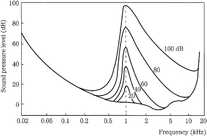
FIGURE 10.7 Masking thresholds vary with respect to sound pressure level. This test uses a narrow-band masker noise centered at 1 kHz. The lower slope remains essentially unchanged.

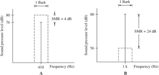
FIGURE 10.8 Noise maskers have more masking power than tonal maskers. A. In NMT, a noise masker can mask a centered tone with an SMR of only 4 dB. B. In TMN, a tonal masker can mask centered noise with an SMR of 24 dB. The SMR increases as the tone or noise moves off the center frequency. In each case, the width of the noise band is one critical bandwidth.

As noted, many masking studies use noise to mask a tone to study the condition called noise-masking-tone (NMT). In perceptual coding, we are often more concerned with quantization noise that must be masked by either a tonal or nontonal (noise-like) audio signal. The conditions of tone-masking-noise (TMN) and noise-masking-noise (NMN) are thus more pertinent. Generally, in noise-masking-tone studies, when the masker and maskee are centered, a tone is inaudible when it is about 4 dB below a 1/3-octave masking noise in a critical band. Conversely, in tone-masking-noise studies, when a 1/3-octave band of noise is masked by a pure tone, the noise must be 21 dB to 28 dB below the tone. This suggests that it is 17 dB to 24 dB harder to mask noise. The two cases are illustrated in Fig. 10.8. NMN generally follows TMN conditions; in one NMN study, the maskee was found to be about 26 dB below the masker. The difference between the level of the masking signal and the level of the masked signal is called the signal-to-mask ratio (SMR); for example, in NMT studies, the SMR is about 4 dB. Higher values for SMR denote less masking. SMR is discussed in more detail below.

Relatively little scientific study has been done with music as the masking stimulus. However, it is generally agreed that music can be considered as relatively tonal or nontonal (noise-like) and these characterizations are used in psychoacoustic models for music coding. The determination of tonal and nontonal components is important because, as noted above, the masking abilities are quite different and this greatly affects coding. In addition, sine-tone masking data is generally used in masking models because it provides the least (worst case) masking of noise; complex tones provide greater masking. Clearly, one musical sound can mask another, but future work in the mechanics of music masking will result in better masking algorithms.

Temporal Masking

Amplitude masking assumes that tones are sounded simultaneously. Temporal masking occurs when tones are sounded close in time, but not simultaneously. A signal can be masked by a noise (or another signal) that occurs later. This is pre-masking (sometimes called backward masking). In addition, a signal can be masked by a noise (or another signal) that ends before the signal begins. This is post-masking (sometimes called forward masking). In other words, a louder masker tone appearing just after (pre-masking), or before (post-masking) a softer tone overcomes the softer tone. Just as simultaneous amplitude masking increases as frequency differences are reduced, temporal masking increases as time differences are reduced. Given an 80-dB tone, there may be 40 dB of post-masking within 20 ms and 0 dB of masking at 200 ms. Pre-masking can provide 60 dB of masking for 1 ms and 0 dB at 25 ms. This is shown in Fig. 10.9. The duration of pre-masking has not been shown to be affected by the duration of the masker. The envelope of post-masking decays more quickly as the duration of the masker decreases or as its intensity decreases. In addition, a tone is better post-masked by an earlier tone when they are close in frequency or when the earlier tone is lower in frequency; post-masking is slight when the masker has a higher frequency. Logically, simultaneous amplitude masking is stronger than either temporal pre- or post-masking because the sounds occur at the same time.

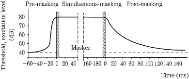
FIGURE 10.9 Temporal masking occurs before and, in particular, after a masker sounds; the threshold decreases with time. The dashed line indicates the threshold for a test-tone impulse without a masker signal. (Zwicker and Zwicker, 1991)

Temporal masking suggests that the brain integrates the perception of sound over a period of time (perhaps 200 ms) and processes the information in bursts at the auditory cortex. Alternatively, perhaps the brain prioritizes loud sounds over soft sounds, or perhaps loud sounds require longer integration times. Whatever the mechanism, temporal masking is important in frequency domain coding. These codecs have limited time resolution because they operate on blocks of samples, thus spreading quantization error over time. Temporal masking can help overcome audibility of the artifact (called pre-echo) caused by a transient signal that lasts a short time while the quantization noise may occupy an entire coding block. Ideally, filter banks should provide a time resolution of 2 ms to 4 ms. Acting together, amplitude and temporal masking form a contour that can be mapped in the time-frequency domain, as shown in Fig. 10.10. Sounds falling under that contour will be masked. It is the obligation of perceptual codecs to identify this contour for changing signal conditions and code the signal appropriately.

Although a maskee signal exists acoustically, it does not exist perceptually. It might seem quite radical, but aural masking is as real as visual masking. Lay your hand over this page. Can you see the page through your hand? Aural masking is just as effective.

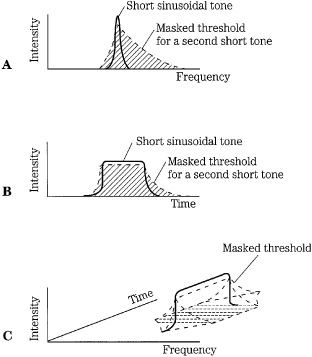
FIGURE 10.10 When simultaneous and temporal masking are combined, a time-frequency contour results. A perceptual codec must place quantization noise and other artifacts within this contour to ensure inaudibility. A. Simultaneous masking. B. Temporal masking. C. Combined masking effect in time and frequency. (Beerends and Stemerdink, 1992)

Psychoacoustic Models

Psychoacoustic models emulate the human hearing system and analyze spectral data to determine how the audio signal can be coded to render quantization noise as inaudible as possible. Most models calculate the masking thresholds for critical bands to determine this just-noticeable noise level. In other words, the model determines how much coding noise is allowed in every critical band, performing one such analysis on each frame of data. The difference between the maximum signal level and the minimum masking threshold (the signal-to-mask ratio) thus determines bit allocation for each band. An important element in modeling masking curves is determining the relative tonality of signals, because this affects the character of the masking curve they project. Any model must be time-aligned so that its results coincide with the correct frame of audio data. This accounts for the filter delay and need to center the analysis output in the current data block.

In most codecs, the goal of bit allocation is to minimize the total noise-to-mask ratio over the entire frame. The number of bits allocated cannot exceed the number of bits available for the frame at a given bit rate. The noise-to-mask ratio for each subband is calculated as:

NMR = SMR − SNR dB

The SNR is the difference between the masker and the noise floor established by a quantization level; the more bits used for quantization, the larger the value of SNR. The SMR is the difference between the masker and the minimum value of the masking threshold within a critical band. More specifically, the pertinent masking threshold is the global masking threshold (also known as the just-noticeable distortion or JND) within a critical band. The SMR determines the number of bits needed for quantization. If a signal is below the threshold, then the signal is not coded. The NMR is the difference between the quantization noise level, and the level where noise reaches audibility. The relationship is shown in Fig. 10.11

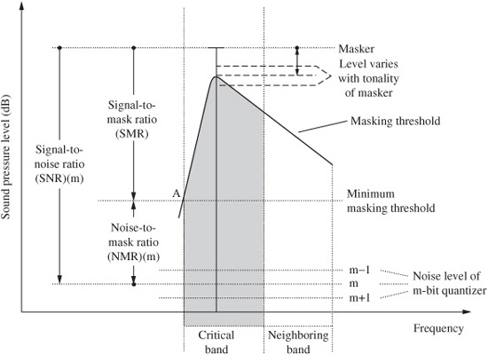
FIGURE 10.11 The NMR is the difference between the SMR and SNR, expressed in dB. The masking threshold varies according to the tonality of the signal. (Noll, 1997)

Within a critical band, the larger the SNR is compared to the SMR, the less audible the quantization noise. If the SNR is less than the SMR, then the noise is audible. A codec thus strives to minimize the value of the NMR in subbands by increasing the accuracy of the quantization. This figure gauges the perceptual quality of the coding. For example, NMR values of less than 0 may indicate transparent coding, while values above 0 may indicate audible degradation.

Referring again to Fig. 10.11, we can also note that the masking threshold is shifted downward from the masking peak by some amount that depends most significantly on whether the masker is tonal or nontonal. Generally, these expressions can be applied:

Δ_TMN = 14.5 + z dB

Δ_NMT = S dB

where z is the frequency in Bark and S can be assumed to lie between 3 and 6 but can be frequency-dependent.

Alternatively, James Johnston has suggested these expressions for the tonalnontonal shift:

Δ_TMN = 19.5 + z(18.0/26.0) dB

Δ_NMT = 6.56 − z(3.06/26.0) dB

where z is the frequency in Bark.

The codec must place noise below the JND, or more specifically, taking into account the absolute threshold of hearing, the codec must place noise below the higher of JND or the threshold of hearing. For example, the SNR may be estimated from table data specified according to the number of quantizing levels, and the SMR is output by the psychoacoustic model. In an iterative process, the bit allocator determines the NMR for all subbands. The subband with the highest NMR value is allocated bits, and a new NMR is calculated based on the SNR value. The process is repeated until all the available bits are allocated.

The validity of the psychoacoustic model is crucial to the success of any perceptual codec, but it is the utilization of the model’s output in the bit allocation and quantization process that ultimately determines the audibility of noise. In that respect, the interrelationship of the model and the quantizer is the most proprietary part of any codec. Many companies have developed proprietary psychoacoustic models and bit-allocation methods that are held in secret; however, their coding is compatible with standards-compliant decoders.

Spreading Function

Many psychoacoustic models use a spreading function to compute an auditory spectrum. It is straightforward to estimate masking levels within a critical band by using a component in the critical band. However, masking is usually not limited to a single critical band; its effect spreads to other bands. The spreading function represents the masking response of the entire basilar membrane and describes masking across several critical bands, that is, how masking can occur several Bark away from a masking signal. In crude models (and the most conservative) the spreading function is an asymmetrical triangle. As noted, the lower slope is about 27 dB/Bark; the upper slope may vary from −20 to −5 dB/Bark. The masking contour of a pure tone can be approximated as two slopes where S₁ is the lower slope and S₂ is the upper slope, plotted as SPL per critical-band rate. The contour is independent of masker frequency:

S₁ = 27 dB / Bark

S₂ = [24 + 0.23(f_v/1000)⁻¹ − 0.2L_v/dB] dB / Bark

where f_v is the frequency of the masking tone in Hz, and L_v is the level of the masking tone in dB.

The slope of S₂ becomes steeper at low frequencies by the 0.23(f_v/1000)⁻¹ term because of the threshold of hearing, while at masking frequencies above 100 Hz, the slope is almost independent of frequency. S₂ also depends on SPL.

A more sophisticated spreading function, but one that does not account for the masker level, is given by the expression:

10 log₁₀ SF(dz) = 15.81 + 7.5(dz + 0.474) − 17.5[1 + (dz + 0.474)²]^1/2 dB

where dz is the distance in Bark between the maskee and masker frequency.

To use a spreading function, the audio spectrum is divided into critical bands and the energy in each band is computed. These values are convolved with the spreading function to yield the auditory spectrum. When offsets and the absolute threshold of hearing are considered, the final masking thresholds are produced. When calculating a global masking threshold, the effects of multiple maskers must be considered. For example, a model could use the higher of two thresholds, or add together the masking threshold intensities of different components. Alternatively, a value averaged between the values of the two methods could be used, or another nonlinear approach could be taken. For example, in the MPEG-1 psychoacoustic model 1, intensities are summed. However, in MPEG-1 model 2, the higher value of the global masking threshold and the absolute threshold is selected. These models are discussed in Chap. 11.

Tonality

Distinguishing between tonal and nontonal components is an important feature of most psychoacoustic models because tonal and nontonal components demand different masking emulation. For example, as noted, noise is a better masker than a tone. Many methods have been devised to detect and characterize tonality in audio signals. For example, in MPEG-1 model 1, tonality is determined by detecting local maxima in the audio spectrum. All nontonal components in a critical band are represented with one value at one frequency. In MPEG-1 model 2, a spectral flatness measure is used to measure the average or global tonality. These models are discussed in Chap. 11.

In some tonality models, when a signal has strong local maxima tonal components, they are detected and withdrawn and coded separately. This flattens the overall spectrum and increases the efficiency of the subsequent Huffman coding because the average number of bits needed in a codebook increases according to the magnitude of the maximum value. The increase in efficiency depends on the nature of the audio signal. Some models further distinguish the harmonic structure of multitonal maskers. With two multitonal maskers of the same power, the one with a strong harmonic structure yields a lower masking threshold.

Identification of tonal and nontonal components can also be important in the decoder when data is conveyed across an error-prone transmission channel and error concealment is applied before the output synthesis filter bank. Missing tonal components can be replaced by predicted values. For example, predictions can be made using an FIR filter for all-pole modeling of the signal, and using an autocorrelation function, coefficients can be generated with the Levinson–Durbin algorithm. Studies indicate that concealment in the lower subbands is more important than in the upper subbands. Noise properly shaped by a spectral envelope can be successfully substituted for missing nontonal sections.

Rationale for Perceptual Coding

The purpose of any low bit-rate coding system is to decrease the data rate, the product of the sampling frequency, and the word length. This can be accomplished by decreasing the sampling frequency; however, the Nyquist theorem dictates a corresponding decrease in high-frequency audio bandwidth. Another approach uniformly decreases the word length; however, this reduces the dynamic range of the audio signal by 6 dB per bit, thus increasing broadband quantization noise. As we have seen, a more enlightened approach uses psychoacoustics. Perceptual codecs maintain sampling frequency, but selectively decrease word length. The word-length reduction is done dynamically based on signal conditions. Specifically, masking and other factors are considered so that the resulting increase in quantization noise is rendered as inaudible as possible. The level of quantization error, and its associated distortion from truncating the word length, can be allowed to rise, so long as it is masked by the audio signal. For example, a codec might convey an audio signal with an average bit rate of 2 bits/sample; with PCM encoding, this would correspond to a signal-to-noise ratio of 12 dB—a very poor result. But by exploiting psychoacoustics, the codec can render the noise floor nearly inaudible.

Perceptual codecs analyze the frequency and amplitude content of the input signal. The encoder removes the irrelevancy and statistical redundancy of the audio signal. In theory, although the method is lossy, the human perceiver will not hear degradation in the decoded signal. Considerable data reduction is possible. For example, a perceptual codec might reduce a channel’s bit rate from 768 kbps to 128 kbps; a word length of 16 bits/sample is reduced to an average of 2.67 bits/sample, and data quantity is reduced by about 83%. Table 10.2 lists various reduction ratios and resulting bit rates for 48-kHz and 44.1-kHz monaural signals. A perceptually coded recording, with a conservative level of reduction, can rival the sound quality of a conventional recording because the data is coded in a much more intelligent fashion, and quite simply, because we do not hear all of what is recorded anyway. In other words, perceptual codecs are efficient because they can convey much of the perceived information in an audio signal, while requiring only a fraction of the data needed by a conventional system.

Part of this efficiency stems from the adaptive quantization used by most perceptual codecs. With PCM, all signals are given equal word lengths. Perceptual codecs assign bits according to audibility. A prominent tone is given a large number of bits to ensure audible integrity. Conversely, fewer bits are used to code soft tones. Inaudible tones are not coded at all. Together, bit rate reduction is achieved. A codec’s reduction ratio (or coding gain) is the ratio of input bit rate to output bit rate. Reduction ratios of 4:1, 6:1, or 12:1 are common. Perceptual codecs have achieved remarkable transparency, so that in many applications reduced data is audibly indistinguishable from linearly represented data. Tests show that reduction ratios of 4:1 or 6:1 can be transparent.

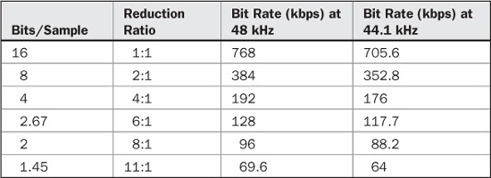
TABLE 10.2 Bit-rate reduction for 48-kHz and 44.1-kHz sampling frequencies.

The heart of a perceptual codec is the bit-allocation algorithm; this is where the bit rate is reduced. For example, a 16-bit monaural signal sampled at 48 kHz that is coded at a bit rate of 96 kbps must be requantized with an average of 2 bits/sample. Moreover, at that bit rate, the bit budget might be 1024 bits per block of analyzed data. The bit-allocation algorithm must determine how best to distribute the bits across the signal’s spectrum and requantize samples to minimize audibility of quantization noise while meeting its overall bit budget for that block.

Generally, two kinds of bit-allocation strategies can be used in perceptual codecs. In forward adaptive allocation, all allocation is performed in the encoder and this encoding information is contained in the bitstream. Very accurate allocation is permitted, provided the encoder is sufficiently sophisticated. An important advantage of forward adaptive coding is that the psychoacoustic model is located in the encoder; the decoder does not need a psychoacoustic model because it uses the encoded data to completely reconstruct the signal. Thus as psychoacoustic models in encoders are improved, the increased sonic quality can be conveyed through existing decoders. A disadvantage is that a portion of the available bit rate is needed to convey the allocation information to the decoder. In backward adaptive allocation, bit-allocation information is derived from the coded audio data itself without explicit information from the encoder. The bit rate is not partly consumed by allocation information. However, because bit allocation in the decoder is calculated from limited information, accuracy may be reduced. In addition, the decoder is more complex, and the psychoacoustic model cannot be easily improved following the introduction of new codecs.

Perceptual coding is generally tolerant of errors. With PCM, an error introduces a broadband noise. However, with most perceptual codecs, the error is limited to a narrow band corresponding to the bandwidth of the coded critical band, thus limiting its loudness. Instead of a click, an error might be perceived as a burst of low-level noise. Perceptual coding systems also permit targeted error correction. For example, particularly vulnerable sounds (such as pianissimo passages) may be given greater protection than less vulnerable sounds (such as forte passages). As with any coded data, perceptually coded data requires error correction appropriate to the storage or transmission medium.

Because perceptual codecs tailor the coding to the ear’s acuity, they may similarly decrease the required response of the playback system itself. Live acoustic music does not pass through amplifiers and loudspeakers—it goes directly to the ear. But recorded music must pass through the playback signal chain. Arguably, some of the original signal present in a recording could degrade the playback system’s ability to reproduce the audible signal. Because a perceptual codec removes inaudible signal content, the playback system’s ability to convey audible music may improve. In short, a perceptual codec may more properly code an audio signal for passage through an audio system.

Perceptual Coding in Time and Frequency

Low bit-rate lossy codecs, whether designed for music or speech coding, attempt to represent the audio signal at a reduced bit rate while minimizing the associated increase in quantization error. Time-domain coding methods such as delta modulation can be considered to be data-reduction codecs (other time-domain methods such as PCM do not provide reduction). They use prediction methods on samples representing the full bandwidth of the audio signal and yield a quantization error spectrum that spans the audio band. Although the audibility of the error depends on the amplitude and spectrum of the signal, the quantization error generally is not masked by the signal. However, time-domain codecs operating across the full bandwidth of the time-domain signal can achieve reduction ratios of up to 2.5. For example, Near Instantaneously Companded Audio Multiplex (NICAM) codecs reduce blocks of 32 samples from 14 bits to 10 bits using a sliding window to determine which 10 of the 14 bits can be transmitted with minimal audible degradation. With this method, coding is lossless with low-level signals, with increasing loss at high levels. Although data reduction is achieved, the bit rate is too high for many applications; primarily, reduction is limited because masking is not fully exploited.

Frequency-domain codecs take a different approach. The signal is analyzed in the frequency domain, and only the perceptually significant parts of the signal are quantized, on the basis of psychoacoustic characteristics of the ear. Other parts of the signal that are below the minimum threshold, or masked by more significant signals, may be judged to be inaudible and are not coded. In addition, quantization resolution is dynamically adapted so that error is allowed to rise near significant parts of the signal with the expectation that when the signal is reconstructed, the error will be masked by the signal. This approach can yield significant data reduction. However, codec complexity is greatly increased.

Conceptually, there are two types of frequency-domain codecs: subband and transform codecs. Generally, subband codecs use a low number of subbands and process samples adjacent in time, and transform codecs use a high number of subbands and process samples adjacent in frequency. Generally, subband codecs provide good time resolution and poor frequency resolution, and transform codecs provide good frequency resolution and poor time resolution.

However, the distinction between subband and transform codecs is primarily based on their separate historical development. Mathematically, all transforms used in codecs can be viewed as filter banks. Perhaps the most practical difference between subband and transform codecs is the number of bands they process. Thus, both subband and transform codecs follow the architecture shown in Fig. 10.12; either time-domain samples or frequency-domain coefficients are quantized according to a psychoacoustic model contained in the encoder.

In subband coding, a hybrid of time- and frequency-domain techniques is used. A short block of time-based broadband input samples is divided into a number of frequency subbands using a filter bank of bandpass filters; this allows determination of the energy in each subband. Using a side-chain transform frequency analysis, the samples in each subband are analyzed for energy content and coded according to a psychoacoustic model.

In transform coding, a block of input samples is directly applied to a transform to obtain the block’s spectrum in the frequency domain. These transform coefficients are then quantized and coded according to a psychoacoustic model. Problematically, a relatively long block of data is required to obtain a high-resolution spectral representation. Transform codecs achieve greater reduction than subband codecs; ratios of 4:1 to 12:1 are typical. Transform codecs incur a longer processing delay than subband codecs.

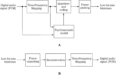
FIGURE 10.12 The basic structure of a time-frequency-domain encoder and decoder (A and B, respectively). Subband (time) codecs quantize time-based samples, and transform (frequency) codecs quantize frequency-based coefficients.

As noted, most low bit-rate lossy codecs use psychoacoustic models to analyze the input signal in the frequency domain. To accomplish this, the time-domain input signal is often applied to a transform prior to analysis in the model. Any periodic signal can be represented as amplitude variations in time, or as a set of frequency coefficients describing amplitude and phase. Jean Baptiste Joseph Fourier first established this relationship between time and frequency. Changes in a time-domain signal also appear as changes in its frequency-domain spectrum. For example, a slowly changing signal would be represented by a low-frequency spectral content. If a sequence of time-based samples are thus transformed, the signal’s spectral content can be determined over that period of time. Likewise, the time-based samples can be recovered by inverse transforming the spectral representation back into the time domain. A variety of mathematical transforms can be used to transform a time-domain signal into the frequency domain and back again. For example, the fast Fourier transform (FFT) gives a spectrum with half as many frequency points as there are time samples. For example, assume that 480 samples are taken at a 48-kHz sampling frequency. In this 10-ms interval, 240 frequency points are obtained over a spectrum from the highest frequency of 24 kHz to the lowest of 100 Hz, which is the period of 10 ms, with frequency points placed 100 Hz apart. In addition, a dc point is generated.

Subband Coding

Subband coding was first developed at Bell Labs in the early 1980s, and much subsequent work was done in Europe later in the decade. Blocks of consecutive time-domain samples representing the broadband signal are collected over a short period and applied to a digital filter bank. This analysis filter bank divides the signal into multiple (perhaps up to 32) bandlimited channels to approximate the critical band response of the human ear. The filter bank must provide a very sharp cutoff (perhaps 100 dB/octave) to emulate critical band response and limit quantization noise within that bandwidth. Only digital filters can accomplish this result. In addition, the processing block length (ideally less than 2 ms to 4 ms) must be small so that quantization error does not exceed the temporal masking limits of the ear. The samples in each subband are analyzed and compared to a psychoacoustic model. The codec adaptively quantizes the samples in each subband based on the masking threshold in that subband. Ideally, the filter bank should yield subbands with a width that corresponds to the width of the narrowest critical band. This would allow precise psychoacoustic modeling. However, most filter banks producing uniformly spaced subbands cannot meet this goal; this points out the difficulties posed by the great difference in bandwidth between the narrowest critical band and the widest.

Each subband is coded independently with greater or fewer bits allocated to the samples in the subband. Quantization noise may be increased in a subband. However, when the signal is reconstructed, the quantization noise in a subband will be limited to that subband, where it is ideally masked by the audio signal in that subband, as shown in Fig. 10.13. Quantization noise levels that are otherwise intrusive can be tolerated in a subband with a signal contained in it because noise will be masked by the signal. Subbands that do not contain an audible signal are quantized to zero. Bit allocation is determined by a psychoacoustic model and analysis of the signal itself; these operations are recalculated for every subband in every new block of data. Samples are dynamically quantized according to audibility of signals and noise. There is great flexibility in the design of psycho-acoustic models and bit-allocation algorithms used in codecs that are otherwise compatible. The decoder uses the quantized data to re-form the samples in each block; a synthesis filter bank sums the subband signals to reconstruct the output broadband signal.

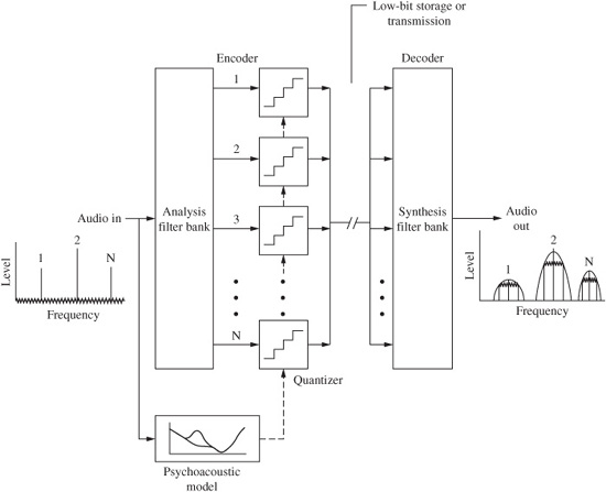
FIGURE 10.13 A subband encoder analyzes the broadband audio signal in narrow subbands. Using masking information from a psychoacoustic model, samples in subbands are coarsely quantized, raising the noise floor. When the samples are reconstructed in the decoder, the synthesis filter constrains the quantization noise floor within each subband, where it is masked by the audio signal.

A subband perceptual codec uses a filter bank to split a short duration of the audio signal into multiple bands, as depicted in Fig. 10.14. In some designs, a side-chain processor applies the signal to a transform such as an FFT to analyze the energy in each subband. These values are applied to a psychoacoustic model to determine the combined masking curve that applies to the signals in that block. This permits more optimal coding of the time-domain samples. Specifically, the encoder analyzes the energy in each subband to determine which subbands contain audible information. A calculation is made to determine the average power level of each subband over the block. This average level is used to calculate the masking level due to masking of signals in each subband, as well as masking from signals in adjacent subbands. Finally, minimum hearing threshold values are applied to each subband to derive its final masking level. Peak power levels present in each subband are calculated, and compared to the masking level. Subbands that do not contain audible information are not coded. Similarly, tones in a subband that are masked by louder nearby tones are not coded, and in some cases entire subbands can mask nearby subbands, which thus need not be coded.

Calculations determine the ratio of peak power to masking level in each subband. Quantization bits are assigned to audible program material with a priority schedule that allocates bits to each subband according to signal strength above the audibility curve. For example, Fig. 10.15 shows vertical lines representing peak power levels, and minimum and masking thresholds.

The signals below the minimum or masking curves are not coded, and the quantization noise floor is allowed to rise to those levels. For example, in the figure, signal A is below the minimum curve and would not be coded in any event. Signal C is also irrelevant in this frame because signal B has dynamically shifted the hearing threshold upward.

Signal B must be coded; however, its presence has created a masking curve, decreasing the relative amplitude above the minimum threshold curve. The portion of signal B between the minimum curve and the masking curve represents the fewer bits that are needed to code the signal when the masking effect is taken into account. In other words, rather than using a signal-to-noise ratio, a signal-to-mask ratio (SMR) is used. The SMR is the difference between the maximum signal and the masking threshold and is used to determine the number of bits assigned to a subband. The SMR is calculated for each subband.

The number of bits allocated to any subband must be sufficient to yield a requantizing noise level that is below the masking level. The number of bits depends on the SMR value, with the goal of maintaining the quantization noise level below the calculated masking level for each subband. In fixed-rate codecs, a bit-pool approach can be taken. A large number of subbands requiring coding and signals with large SMR values might empty the pool, resulting in less than optimal coding. On the other hand, if the pool is not empty after initial allocation, the process is repeated until all bits in the codec’s data capacity have been used. Typically, the iterative process continues, allocating more bits where required, with signals with the highest SMR requirements always receiving the most bits; this increases the coding margin. In some cases, subbands previously classified as inaudible might receive coding from these extra bits. Thus, signals below the masking threshold can in practice be coded, but only on a secondary priority basis. Summarizing the concept of subband coding, Fig. 10.16 shows how a 24-subband codec might code three tones at 250 Hz, 1 kHz, and 4 kHz; note that in each case the quantization noise level is below the combined masking and threshold curve.

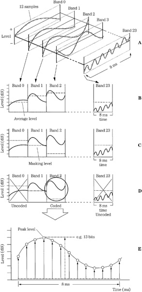
FIGURE 10.14 A subband codec divides the signal into narrow subbands, calculates average signal level, and masking level; and then quantizes the samples in each subband accordingly. A. Output of 24-band subband filter. B. Calculation of average level in each subband. C. Calculation of masking level in each subband. D. Subbands below audibility are not coded; bands above audibility are coded. E. Bits are allocated according to peak level above the masking threshold. Subbands with peak levels above the masking level contain audible signals that must be coded.

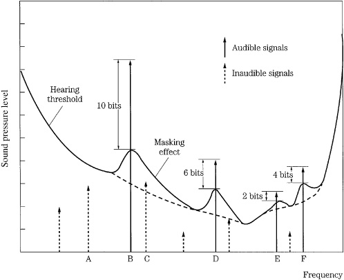
FIGURE 10.15 The bit-allocation algorithm assigns bits according to audibility of subband signals. Bits may not be assigned to masked or inaudible tones.

Transform Coding

In transform coding, the audio signal is viewed as a quasi-stationary signal that changes relatively little over short time intervals. For efficient coding, blocks of time-domain audio samples are transformed to the frequency domain. Frequency coefficients, rather than amplitude samples, are quantized to achieve data reduction. For playback, the coefficients are inverse-transformed back to the time domain.

The operation of the transform approximates how the basilar membrane analyzes the frequency content of vibrations along its length. The spectral coefficients output by the transform are quantized according to a psychoacoustic model; masked components are eliminated, and quantization decisions are made based on audibility. In contrast to a subband codec, which uses frequency analysis to code time-based samples, a transform codec codes frequency coefficients. From an information theory standpoint, the transform reduces the entropy of the signal, permitting efficient coding. Longer transform blocks provide greater spectral resolution, but lose temporal resolution; for example, a long block might result in a pre-echo before a transient. In many codecs, block length is adapted according to audio signal conditions. Short blocks are used for transient signals, while long blocks are used for continuous signals.

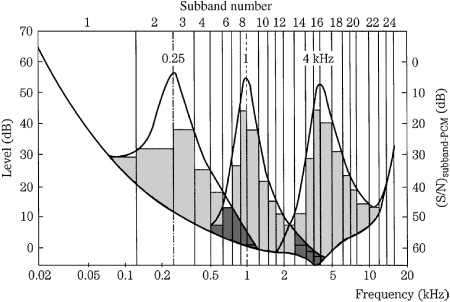
FIGURE 10.16 In this 24-band subband codec, three tones are coded so that the quantization noise in each subband falls below the calculated composite masking curves. (Thiele, Link, and Stoll, 1987)

Time-domain samples are transformed to the frequency domain, yielding spectral coefficients. The coefficient numbers are sometimes called frequency bin numbers; for example, a 512-point transform can produce 256 frequency coefficients or frequency bins. The coefficients, which might number 512, 1024, or more, are grouped into about 32 bands that emulate critical-band analysis. This spectrum represents the block of time-based input samples. The frequency coefficients in each band are quantized according to the codec’s psychoacoustic model; quantization can be uniform, nonuniform, fixed, or adaptive in each band.

Transform codecs may use a discrete cosine transform (DCT) or modified discrete cosine transform (MDCT) for transform coding because of low computational complexity, and because they can critically sample (sample at twice the bandwidth of the bandpass filter) the signal to yield an appropriate number of coefficients. Most codecs overlap successive blocks in time by about 50%, so that each sample appears in two different transform blocks. For example, the samples in the first half of a current block are repeated from the second half of the previous block. This reduces changes in spectra from block to block and improves temporal resolution. The DCT and MDCT can yield the same number of coefficients as with non-overlapping blocks. As noted, an FFT may be used in the codec’s side chain to yield coefficients for perceptual modeling.

All low bit-rate codecs operate over a block of samples. This block must be kept short to stay within the temporal masking limits of the ear. During decoding, quantization noise will be spread over the frequency of the band, and over the duration of the block. If the block is longer than temporal backward masking allows, the noise will be heard prior to the onset of the sound, in a phenomenon known as pre-echo. (The term pre-echo is misleading.) Pre-echo is particularly problematic in the case of a silence followed by a time-domain transient within the analysis window. The energy in the transient portion causes the encoder to allocate relatively few bits, thus raising the eventual quantization noise level. Pre-echoes are created in the decoder when frequency coefficients are inverse-transformed prior to the reconstruction of subband samples in the synthesis filter bank. The duration of the quantization noise equals that of the synthesis window, so the elevated noise extends over the duration of the window, while the transient only occurs briefly. In other words, encoding dictates that a transient in the audio signal will be accompanied by an increase in quantization noise but a brief transient may not fully mask the quantization noise surrounding it, as shown in Fig. 10.17. In this example, the attack of a triangle occurs as a transient signal. The analysis window of a transform codec operates over a relatively long time period. Quantization noise is spread over the time of the window and precedes the music signal; thus it may be audible as a pre-echo.

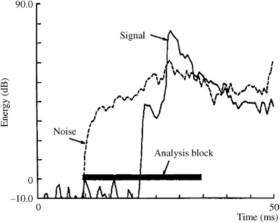
FIGURE 10.17 An example of a pre-echo. On reconstruction, quantization noise falls within the analysis block, where the leading edge is not masked by the signal. (Herre and Johnston, 1996)

Transform codecs are particularly affected by the problem of pre-echo because they require long blocks for greater frequency accuracy. Short block length limits frequency resolution (and also relatively increases the amount of overhead side information). In essence, transform codecs sacrifice temporal resolution for spectral resolution. Long blocks are suitable for slowly changing or tonal signals; the frequency resolution allows the codec to identify spectral peaks and use their masking properties in bit allocation. For example, a clarinet note and its harmonics would require fine frequency resolution but only coarse time resolution. However, transient signals require a short block length; the signals have a flatter spectrum. For example, the fast transient of a castanet click would require fine time resolution but only coarse frequency resolution.

In most transform codecs, to provide the resolution demanded by particular signal conditions, and to avoid pre-echo, block length dynamically adapts to signal conditions. Referring again to Fig. 10.17, a shorter analysis block would constrain the quantization noise to a shorter duration, where it will be masked by the signal. A short block is also advantageous because it limits the duration of high bit rates demanded by transient encoding. Alternatively, a variable bit rate encoder can minimize pre-echo by briefly increasing the bit rate to decrease the noise level. Some codecs use temporal noise shaping (TNS) to minimize pre-echo by manipulating the nature of the quantization noise within a filter bank window. When a transient signal is detected, TNS uses a predictive coding method to shape the quantization noise to follow the transient’s envelope. In this way, the quantization error is more effectively concealed by the transient. However, no matter what approach is taken, difficulty arises because most music simultaneously places contradictory demands on the codec.

In adaptive transform codecs, a model is applied to uniformly and adaptively quantize each individual band, but coefficient values within a band are quantized with the same number of bits. The bit-allocation algorithm calculates the optimal quantization noise in each subband to achieve a desired signal-to-noise ratio that will promote masking. Iterative allocation is used to supply additional bits as available to increase the coding margin, yet maintain limited bit rate. In some cases, the output bit rate can be fixed or variable for each block. Before transmission, the reduced data is often compressed with entropy coding such as Huffman coding and run-length coding to perform lossless compression. The decoder inversely quantizes the coefficients and performs an inverse transform to reconstruct the signal in the time domain.

An example of an adaptive transform codec proposed by Karlheinz Brandenburg is shown in Fig. 10.18. An MDCT transforms the signal to the frequency domain. Signal energy in each critical band is calculated using the spectral coefficients. This is used to determine the masking threshold for each critical band. Two iterative loops perform quantization and coding using an analysis-by-synthesis technique. Coefficients are initially assigned a quantizer step size and the algorithm calculates the resulting number of bits needed to code the signal in the block. If the count exceeds the bit rate allowed for the block, the loop reassigns a larger quantizer step size and the count is recalculated until the target bit rate is achieved. An outer loop calculates the quantization error as it will appear in the reconstructed signal. If the error in a band exceeds the error allowed by the masking model, the quantizer step size in the band is decreased. Iterations continue in both loops until optimal coding is achieved. Codecs such as this can operate at low bit rates (for example, 2.5 bits/sample).

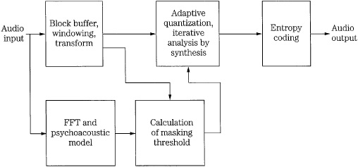
FIGURE 10.18 Adaptive transform codec using an FFT side-chain and iterative quantization to achieve optimal reduction. Entropy coding is additionally used for data compression.

Filter Banks

Low bit-rate codecs often use an analysis filter bank to partition the wide audio band into smaller subbands; the decoder uses a synthesis filter bank to restore the subbands to a wide audio band. Uniformly spaced filter banks downconvert an audio band into a baseband, then lowpass filter and subsample the data. Transform-based filter banks multiply overlapping blocks of audio samples with a window function to reduce edge effects, and then perform a discrete transform such as DCT. Mathematically, the transforms used in codecs can be seen as filter banks, and subband filter banks can be seen as transforms.

Time-domain filter banks should provide ideal lowpass and highpass characteristics with a cutoff of f_s/2, where f_s is the sampling frequency; however, real filters have overlapping bands. For example, in a two-band system, the subband sampling rates must be decreased (2:1) to maintain the overall bit rate. This decimation introduces aliasing in the subbands. In the lower band, signals above f_s/4 will alias to 0 to f_s/4. In the upper band, signals below f_s/4 alias up to f_s/4 to f_s/2. In the decoder, the sampling rate is restored (1:2) by adding zeros. Because of interpolation, in the lower band, signals from 0 to f_s/4 will image around f_s/4 into the upper band. Similarly, in the upper band, signals from f_s/4 to f_s/2 will image to the lower band.

Quadrature Mirror Filters

Generally, when N subbands are created, each subband is sub-sampled at 1/N to maintain an overall sampling limit. We recall from Chap. 2, that the sampling frequency must be at least twice the bandwidth of a sampled signal. As noted, most filter banks do not provide ideal performance because of the finite width of their transition bands; the bands overlap, and the 1/N sub-sampling causes aliasing. Clearly, bands that are spaced apart can avoid this, but will leave gaps in the signal’s spectrum. Quadrature mirror filter (QMF) banks have the property of reconstructing the original signal from N overlapping subbands without aliasing, regardless of the order of the bandpass filters. The aliasing components are exactly canceled, in the frequency domain, during reconstruction and the subbands are output in their proper place in frequency. The attenuation slopes of adjacent subband filters are mirror images of each other. Ideally, alias cancellation is perfect only if there is no requantization of the subband signals. A QMF is shown in Fig. 10.19. Intermediate samples can be critically sub-sampled without loss; if the input signal is split into N equal subbands, each subband can be sampled at 1/N; the sampling frequency for each subband filter is exactly twice the bandwidth of the filter. Generally, cascades of QMF banks may be used to create 4 to 24 subbands. By cascading some subbands unequally, relative bandwidths can be manipulated; delays are introduced to maintain time parity between subbands.

QMF banks can be implemented as symmetrical finite impulse-response filters with an even number of taps; the use of a reconstruction highpass filter with a z-transform of −H(−z) instead of H(−z) eliminates alias terms (when there is uniform quantizing in each subband). However, perfect reconstruction is generally limited to the case when N = 2, creating two equal-width subbands from one. These f_s/2 subbands can be further divided by repeating the QMF process, and splitting each subband into two more subbands, each with a f_s/4 sampling frequency. This can be accomplished with a tree structure; however, this adds delay to the processing. Other QMF architectures can be used to create multiple subbands with less delay. However, cascaded QMF banks suitable for multi-band computation needed for codec design suffer from long delay and high complexity. For that reason, many codecs use a pseudo-QMF, also known as a polyphase filter, which offers a faster parallel approach that approximates the QMF. The QMF method is similar in concept to wavelet techniques.

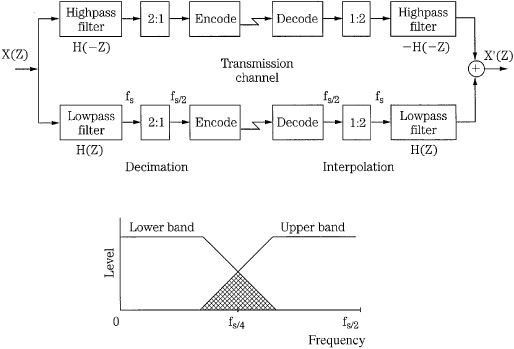
FIGURE 10.19 A quadrature mirror filter forms two equal subbands. Alias components introduced during decimation are exactly canceled during reconstruction. Multiple QMF stages can be cascaded to form additional subbands.

Hybrid Filters

As noted, although filter banks with equally spaced bands are often used, they do not correlate well with the spacing of the ear’s critical bands. Tree-structured filter banks can overcome this drawback. An example of a hybrid filter bank proposed by Karlheinz Brandenburg and James Johnston is shown in Fig. 10.20. It provides frequency analysis that corresponds more closely to critical-band spacing. Time-domain samples are applied to an 80-tap QMF filter bank to yield four bands with bandwidths of 3 kHz, 6 kHz, and 12 kHz. The bands are applied to a 64-line transform that is sine-windowed with a 50% overlap. The output of 320 spectral components has a frequency resolution of 23.4 Hz at low frequencies and 187.5 Hz at high frequencies. A corresponding synthesis filter is used in the decoder.

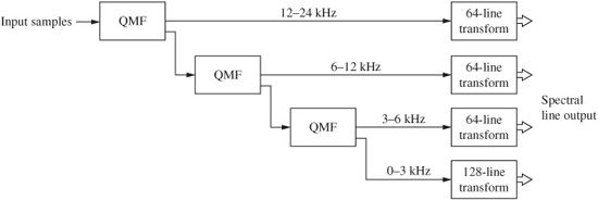
FIGURE 10.20 A hybrid filter using a QMF filter bank and transforms to yield unequally spaced spectral components. (Brandenburg and Johnston, 1990)

Polyphase Filters

A polyphase filter (also known as a pseudo-QMF or PQMF) yields a set of equally spaced bandwidth filters with phase interrelationships that permit very efficient implementation. A polyphase filter bank can be implemented as an FIR filter that consolidates interpolation filtering and decimation. The different filters are generated from a single lowpass prototype FIR filter by modulating the prototype filter over different phases in time. For example, using a 512-tap FIR filter, each block of input samples uses 32 sets of coefficients to create 32 subbands, as shown in Fig. 10.21. More generally, in an N-phase filter bank, each of the N subbands is decimated to a sampling frequency of 1/N. For every N input, the filter outputs one value in each subband. In the first phase, the samples in an FIR transversal register and first-phase coefficients are used to compute the value in the first subband. In the second phase, the same samples in the register and second-phase coefficients are used to compute the value in the second subband, and so on. The impulse response coefficients in the first phase represent a prototype lowpass filter, and the coefficients in the other subband phases are derived from the prototype by multiplication with a cosine modulating function that shifts the low-pass response to each next bandpass center frequency. After N samples are output, the samples in the register are shifted by N, and the process begins again. The center frequencies f_c are given by:

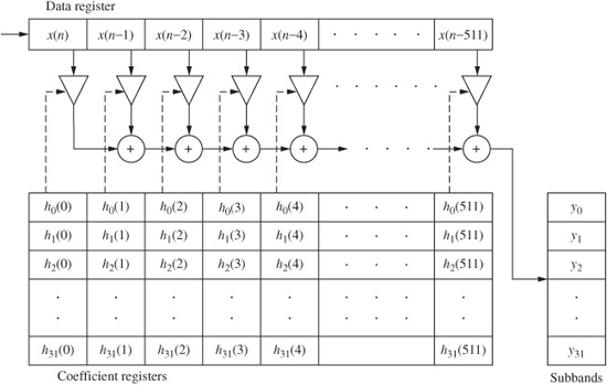
FIGURE 10.21 A polyphase filter uses a single lowpass prototype FIR filter to create subbands by modulating the prototype filter. This example shows a 512-tap filter with 32 sets of 512 coefficients, yielding 32 subbands.

f_c = ± f_s(k + 1/2)/2N Hz

where f_s is the sampling frequency and N is the number of subbands and k = 0, 1, 2, … , N−1.

Each subband has a bandwidth of f_s/64. Polyphase filter banks offer good time-domain resolution, and good frequency resolution that can yield high stopband attenuation of 96 dB to minimize intraband aliasing. There is significant overlap in adjacent bands, but phase shifts in the cosine terms yield frequency-domain alias cancellation at the synthesis filter. The quantization process slightly degrades alias cancellation. The MPEG-1 and -2 standards specify a polyphase filter with QMF characteristics, operating as a block transform with N = 32 subbands and a 512-tap register. The flow chart of the MPEG-1 analysis filter and other details are given in Chap. 11. The particular analysis filter presented in the MPEG-1 standard requires approximately 80 real multiplies and 80 real additions for every output sample. Similarly, a polyphase synthesis filter is used in the decoder. The PQMF is a good choice to create a limited number of frequency bands. When higher-resolution analysis is needed, approaches such as an MDCT transform are preferred.

MDCT

The discrete Fourier transform (DFT) and discrete cosine transform (DCT) could be used in codecs to provide good frequency resolution. Also, the number of output points in the frequency domain equals the number of input samples in the time domain. However, to reduce blocking artifacts, an overlap-and-add of 50% doubles the number of frequency components relative to the number of time samples, and the DFT and DCT do not provide critical sampling. The increase in data rate is clearly counterproductive. The modified discrete cosine transform (MDCT) provides high-resolution frequency analysis and can allow a 50% overlap and provide critical sampling. As a result, it is used in many codecs.

The MDCT is an example of a time-domain aliasing cancellation (TDAC) transform in which only half of the frequency points are needed to reconstruct the time-domain audio signal. Frequency-domain sub-sampling is performed; thus, a 50% overlap results in the same number of output points as input samples. Specifically, the length of the overlapping windows is twice that of the block time (shift length of the transform) resulting in a 50% overlap between blocks. Moreover, the overlap-and-add process is designed to cancel time-domain aliasing and allow perfect reconstruction. The MDCT also allows adaptability of filter resolution by changing the window length. Windows such as a sine taper and Kaiser–Bessel can be used. The MDCT also lends itself to adaptive window switching approaches with different window functions for the first and second half of the window; the time-domain aliasing property must be independently valid for each window half. Many bands are possible with the MDCT with good efficiency, on the order of an FFT computation. The MDCT is also known as the modulated lapped transform (MLT).

As noted, a window function is applied to blocks of samples prior to transformation. If a block is input to a filter bank without a window, it can be considered as a time-limited signal with a rectangular window in which the samples in the block are multiplied by 1 and all other samples are multiplied by 0. The Fourier transform of this signal reveals that the sharp cutoff of the window’s edges yields high-frequency content that would cause aliasing. To minimize this, a window can be applied that tapers the time-domain edge response down to zero. A window is thus a time function that is multiplied by an audio block to provide a windowed audio block. The window shape is selected to balance high-frequency resolution of the filter bank while minimizing spurious spectral components. The effect of the window must be compensated for to recover the original input signal after inverse-transformation. The overlap-and-add procedure accomplishes this by overlapping windowed blocks of the input signal and adding the result. The windows are designed specifically to allow this. Digital filters and windows are discussed in Chap. 17.

As noted, hybrid filter banks use a cascade of different filter types (such as polyphase and MDCT) to provide different frequency resolutions at different frequencies with moderate complexity. For example, MPEG-1 Layer III encoders use a hybrid filter with a polyphase filter bank and MDCT. The ATRAC algorithm is a hybrid codec that uses QMF to divide the signal into three subbands, and each subband is transformed into the frequency domain using the MDCT. Table 10.3 compares the properties of filter banks used in several low bit-rate codecs.

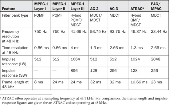
TABLE 10.3 Comparison of filter-bank properties (48-kHz sampling frequency). (Brandenburg and Bosi, 1997)

Multichannel Coding

The problem of masking quantization noise is straightforward with a monaural audio signal; the masker and maskee are co-located. However, stereo and surround audio content also contain spatial localization cues. As a consequence, multichannel playback presents additional opportunities and obligations for low bit-rate algorithms. On one hand, for example, interchannel redundancies can be exploited by the coding algorithm to additionally and significantly reduce the necessary bit rate. On the other hand, great care must be taken because masking is spatially dependent. For example, quantization noise in one channel might be unmasked because its spatial placement differs from that of a masking signal in another channel. The human ear is fairly acute at spatial localization; for example, with the “cocktail-party effect” we are able to listen to one voice even when surrounded by a room filled with voices. The unmasking problem is particularly challenging because most masking studies assume monaural channels where the masker and maskee are spatially equal. In addition, perceptual effects are very different for loudspeaker versus headphone playback.

At frequencies above 2 kHz, within critical bands, we tend to localize sounds based on the temporal envelope of the signal rather than specific temporal details. Coding artifacts must be concealed in time and frequency, as well as in space. If stereo channels are improperly coded, coding characteristics of one channel might interfere with the other channel, creating stereo unmasking effects. For example, if a masking sum or difference signal is incorrectly processed in a matrixing operation and is output in the wrong channel, the noise in its original channel that it was supposed to mask might become audible.

Dual-mono coding uses two codecs operating independently. Joint-mono coding uses two monophonic codecs but they operate under the constraint of a single bit rate. Independent coding of multiple channels can create coding artifacts. For example, quantization noise might be audibly unmasked because it does not match the spatial placement of a stereo masking signal. Multichannel coding must consider subtle changes in the underlying psychoacoustics. For example, with the binaural masking level difference (BMLD) phenomenon, the masking threshold can be lower when listening with two ears, instead of one. At low frequencies (below 500 Hz), differences in phase between the masker and maskee at two ears can be readily audible.

Joint-stereo coding techniques use interchannel properties to take advantage of interchannel redundancy and irrelevance between stereo (or multiple) channels to increase efficiency. The data rate of a stereo signal is double that of a monaural signal, but most stereo programs are not dual-mono. For example, the channels usually share some level and phase information to create phantom images. This interchannel correlation is not apparent in the time domain, but it is readily apparent when analyzing magnitude values in the frequency domain. Joint-stereo coding codes common information only once, instead of twice as in left/right independent coding. A 256-kbps joint-stereo coding channel will perform better than two 128-kbps channels.

Many multichannel codecs use M/S (middle/side) coding of stereo signals to eliminate redundant monaural information. Coding efficiency can be high particularly with near-monaural signals and the technique performs well when there is a BMLD. With the M/S technique, rather than code discrete left and right channels, it is more efficient to code the middle (sum) and side (difference) signals using a matrix in either the time or frequency domains. The decoder uses reverse processing. In a multichannel codec, M/S coding can be applied to channel pairs placed left/right symmetrically to the listener. This configuration helps to avoid spatial unmasking.

As an alternative to M/S coding, intensity stereo coding (also known as dynamic crosstalk or channel coupling) can be used. High frequencies are primarily perceived as energy-time envelopes. With the intensity stereo technique, the energy-time envelope is coded rather than the waveform itself. One set of values can be efficiently coded and shared among multiple channels. Envelopes of individual channels can be reconstructed in the decoder by individually applying proper amplitude scaling. The technique is particularly effective at coding spatial information. In some codecs, different joint-stereo coding techniques are used in different spectral areas.

Using diverse and dynamically changing psychoacoustic cues and signal analysis, inaudible components can be removed with acceptable degradation. For example, a loud sound in one loudspeaker channel can mask other softer sounds in other channels. Above 2 kHz, localization is achieved primarily by amplitude; because the ear cannot follow fast individual waveform cycles, it tracks the envelope of the signal, not its phase. Thus the waveform itself becomes less critical; this is intensity localization. In addition, the ear is limited in its ability to localize sounds close in frequency. To convey a multichannel surround field, the high frequencies in each channel can be divided into bands and combined band by band into a composite channel. The bands of the common channel are reproduced from each loudspeaker, or panned between loudspeakers, with the original signal band envelopes. Use of a composite channel achieves data reduction. In addition, other masking principles can be applied prior to forming the composite channel. Many multichannel systems use a 5.1 format with three front channels, two independent surround channels, and a subwoofer channel. Very generally, the number of bits required to code a multichannel signal is proportional to the square root of the number of channels. A 5.1-channel codec, for example, would theoretically require only 2.26 times the number of bits needed to code one channel.

Tandem Codecs

In many applications, perceptual codecs will be used in tandem (cascaded). For example, a radio station may receive a coded signal, decode it to PCM for mixing, crossfading, and other operations, and then code it again for broadcast, where it is decoded by the consumer, who may make a coded recording of it. In all, many different coding processes may occur. As the signal passes through this chain, coding artifacts will accumulate and can become audible. The nature of the signal degrades the ability of subsequent codecs to suitably model the signal. Each codec will quantize the audio signal, adding to the quantization noise already permitted by previous encoders. Because many psychoacoustic models monitor the audio masking levels and not the underlying noise, noise can be allowed to rise to the point of audibility. Furthermore, when noise reaches audibility, the codec may allocate bits to code it, thus robbing bits needed elsewhere; this can increase noise in other areas.

In addition, tandem codecs are not necessarily synchronized, and will delineate audio data frames differently. This can yield audible noise-like artifacts and pre-echoes in the signal. When codecs are cascaded, it is important to begin with the highest-quality coding possible, then step down. A low-fidelity link will limit all subsequent processing. Highest-quality codecs have a high coding margin between the masking threshold, and coding noise; they tolerate more coding generations.

To reduce degradation caused by cascading, researchers are developing “inverse decoders” that analyze a decoded low bit-rate bitstream and extract the encoding parameters used to encode it. If the subsequent encoder is given the relevant coding decisions used by the previous encoder, and uses the same quantization parameters, the signal can be re-encoded very accurately with minimal loss compared to the first-generation coded signal. Conceivably, aspects such as type of codec, filter bank type, framing, spectral quantization, and stereo coding parameters can be extracted. Further, such systems could use the extracted parameters to ideally re-code the signal to its original bitstream representation, thus avoiding the distortion accumulated by repeatedly encoding/decoding content through the cascades in a signal chain. Some systems would accomplish this analysis and reconstruction task using only the decoded audio bitstream.

In some codec designs, metadata, sometimes called “mole” data because it is buried data that can burrow through the signal chain, is embedded in the audio data using steganographic means. Mole data such as header information, frame alignment, bit allocation, and scale factors may be conveyed. The mole data helps ensure that cascading does not introduce additional distortion. Ideally, the auxiliary information allows subsequent codecs to derive all the encoding parameters originally used in the first-generation encoding. This lets downstream tandem codecs apply the same framing boundaries, psychoacoustic modeling, and quantization processing as upstream stages. It is particularly important for the inverse decoder to use the same frame alignment as the original encoder so that the same sets of samples are available for processing.

With correct parameters, the cascaded output coded bitstream may be nearly identical to the input coded bitstream, within the tolerances of the filter banks. In another effort to reduce the effects of cascading, some systems allow operations to take place on the signal in the codec domain, without need for intermediate decoding to PCM and re-encoding. Such systems may allow gain-changing, fade-in and fade-outs, cross-fading, equalization, transcoding to a higher or lower bit rate, and transcoding to a different codec, as the signal passes through a signal chain.

Spectral Band Replication

Any perceptual codec must balance audio bandwidth, bit rate, and audible artifacts. By reducing coded audio bandwidth, relatively more bits are available in the remaining bandwidth. Spectral band replication (SBR) allows the underlying codec to reduce bit rate through bandwidth reduction, while providing bandwidth extension at the decoder. Spectral band replication is primarily a postprocess that occurs at the receiver. It extends the high-frequency range of the audio signal at the receiver. The lower part of the spectrum is transmitted. Higher frequencies are reconstructed by the SBR decoder based on the lower transmitted frequencies and control information. The replicated high-frequency signal is not analytically coherent compared to the baseband signal, but is coherent in a psychoacoustic sense; this is assisted by the fact that the ear is relatively less sensitive to variations at high frequencies.

The codec operates at half the nominal sampling frequency while the SBR algorithm operates at the full sampling frequency. The SBR encoder precedes the waveform encoder and uses QMF analysis and energy calculations to extract information that describes the spectral envelope of the signal by measuring energy in different bands. This process must be uniquely adaptive to its time and frequency analysis. For example, a transient signal might exhibit significant energy in the high band, but much less in the low band that will be conveyed by the codec and used for replication. The encoder also compares the original signal to the signal that the decoder will replicate. For example, tonal and nontonal aspects and the correlation between the low and high bands are analyzed. The encoder also considers what frequency ranges the underlying codec is coding. To assist the processing, control information is transmitted by the encoded bitstream at a very low bit rate. SBR can be employed for monaural, stereo, or multichannel encoding.

The SBR decoder follows the waveform decoder and uses the time-domain signal decoded by the underlying codec. This lowpass data is upsampled and applied to a QMF analysis filter bank and its subband signals (perhaps 32) are used for high-band replication based on the control information. In addition, the replicated high-band data is adaptively filtered and envelopment adjustment is applied to achieve suitable perceptual characteristics. The delayed low-band and high-band subbands are applied to a synthesis filter bank (perhaps 64 bands) operating at the SBR sampling frequency. In some cases, the encoder measures stereo correlation in the original signal and the decoder generates a corresponding pseudo-stereo signal. Replicated spectral components must be harmonically related to the baseband components to avoid dissonance.

At low and medium bit rates, SBR can improve the efficiency of a perceptual codec by as much as 30%. The improvement depends on the type of codec used. For example, when SBR is used with MP3 (as in MP3PRO), a 64-kbps stereo stream can achieve quality similar to that of a conventional MP3 96-kbps stereo stream. Generally, SBR is most effective when the codec bit rate is set to provide an acceptable level of artifacts in the restricted bandwidth. MP3PRO uses SBR in a backward- and forward-compatible way. Conventional MP3 players can decode an MP3PRO bitstream (without SBR) and MP3PRO decoders can decode MP3 and MP3PRO streams. SBR techniques can also be applied to Layer II codecs and MPEG-4 AAC codecs; the latter application is called High-Efficiency AAC (HE AAC) and aacPlus.

Low-complexity SBR can be accomplished with “blind” processing in which the decoder is not given control information. A nonlinear device such as a full-wave rectifier is used to generate harmonics, a filter selects the needed part of the signal, and gain is adjusted. This method assumes correlation between low- and high-frequency bands, thus its reconstruction is relatively inexact. Other SBR methods may extend low-frequency audio content by generating subharmonics, for example, in a voice signal passing through a telephone system that is bandlimited at low frequencies (as well as high frequencies). Other SBR methods are specifically designed to enhance sound quality through small loudspeakers. For example, a system might shift unreproducible low frequencies to higher frequencies above the speaker’s cutoff, and rely on psycho-acoustic effects such as residue pitch and virtual pitch to create the impression of low-frequency content.

Perceptual Coding Performance Evaluation

Whereas traditional audio coding is often a question of specifications and measurements, perceptual coding is one of physiology and perception. With the advent of digital signal processing, audio engineers can design hardware and software that “hears” sound the same way that humans hear sound.

The question of how to measure the sonic performance of perceptual codecs raises many issues that were never faced by traditional audio systems. Linear measurements might reveal some limitations, but cannot fully penetrate the question of the algorithm’s perceptual accuracy. For example, a narrow band of noise introduced around a tone might not be audible, broadband white noise at the same energy would be plainly audible, but both would provide the same signal-to-noise measurement. Demonstrations of the so-called “13-dB miracle” by James Johnston and Karlheinz Brandenburg showed how noise that is shaped to hide under a narrow-band audio signal can be just barely noticeable or inaudible, yet the measured signal-to-noise ratio is only 13 dB. However, a wideband noise level with an S/N ratio of 60 dB in the presence of the same narrow-band audio signal would be plainly audible. As another example, a series of sine tones might provide a flat frequency response in a perceptual codec because the tones are easily coded. However, a broadband complex tone might be coded with a signal-dependent response.

Traditional audio devices are measured according to their small deviations from linearity. Perceptual codecs are highly nonlinear, as is their model, the human ear. The problem of how to determine the audibility of quantization noise levels and coding artifacts is not trivial. Indeed, the entire field of psychoacoustics must wrestle with the question of whether any objective or subjective measures can wholly quantify how an audible event affects a complex biological system—that is, a listener.

It is possible to nonquantitatively evaluate reduction artifacts using simple test equipment. A sine-wave oscillator can output test tones at a variety of frequencies; a dual-trace oscilloscope can display both the uncompressed and compressed waveforms. The waveforms should be time-aligned to compensate for processing delay in the codec. With a 16-bit system, viewed at 2 V peak-to-peak, one bit represents 30 μV. Any errors, including wideband noise and harmonic distortion at the one-bit level, can be observed. The idle channel signal performance can be observed with the coded output of a zero input signal; noise, error patterns, or glitches might appear. It also might be instructive to examine a low-level signal (0.1 V). In addition, a maximum level signal can be used to evaluate headroom at a variety of frequencies. More sophisticated evaluation can be performed with distortion and spectrum analyzers, but analysis is difficult. For example, traditional systems can be evaluated by measuring total harmonic distortion and noise (THD + N or SINAD) but such measurements are not meaningful for perceptual codecs. Figure 10.22 shows the spectral analysis of a 16-bit linear recorder and a 384-kbps perceptual recorder. When encoding a simple sine wave, although the perceptual codec adds noise within its masking curve around the tone, it easily codes the signal with low distortion. When using more complex stimuli, a perceptual codec will generate high distortion and noise measurements as anticipated by its inherent function. But, such measurements have little correlation to subjective performance. Clearly, traditional test tones and measurements are of limited use in evaluating perceptual codecs.

Richard Cabot devised a test that perceptually compares the codec output with a known steady-state test signal. A multi-tone signal is applied to the codec; the output is transformed into the frequency domain with FFT, and applied to an auditory model to estimate masking effects of the signal. Because the spectrum of the test signal is known, any error products can be identified and measured. In particular, the error signal can be compared to internally modeled masking curves to estimate audibility. The NMR of the error signal level and masking threshold can be displayed as a function of frequency.

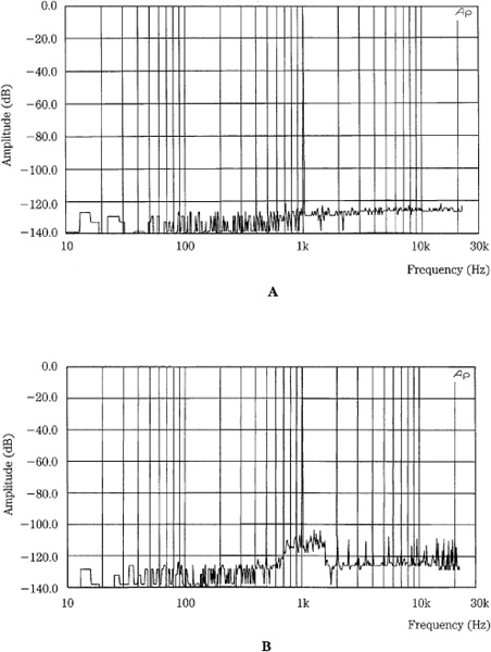
FIGURE 10.22 Spectral analysis of a single 1-kHz test tone reveals little about the performance of a perceptual codec. A. Analysis of a 16-bit linear PCM signal shows a noise floor that is 120 dB below signal. B. Analysis of a 384-kbps perceptually coded signal shows a noise floor that is 110 dB below signal with a slightly increased noise within the masking curve.

For example, Fig. 10.23A shows a steady-state test of a codec. The multi-tone signal consists of 26 sine waves distributed logarithmically across the audio spectrum, approximately one per critical band with a gap to allow for analysis of residual noise and distortion. It is designed to maximally load the codec’s subbands, and consume its available bit rate. The figure shows the modeled masking curve based on the multi-tone, and distortion produced by the codec, consisting of quantization error, intermodulation products, and noise sidebands. In Fig. 10.23B, the system has also integrated the distortion and noise products across the critical bandwidth of the human ear to simulate a perceived distortion level. Distortion products above the model’s masking curve might be audible, depending on ambient listening conditions. In this case, some distortion might be audible at low levels. Clearly, evaluation of results depends on the sophistication of the analyzer’s masking model. Multichannel test tones can be used to analyze interchannel performance, for example, to determine how high frequency information is combined between channels. This particular test does not evaluate temporal artifacts.

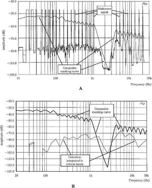
FIGURE 10.23 A multi-tone test signal is designed to deplete the bit capacity of a perceptual codec, emulating the action of a complex musical tone. A. Analysis shows the output test tone and the composite masking curve calculated by the testing device. B. The testing device computes the composite distortion in critical bands. Distortion above the calculated masking threshold might be audible.

Theoretically, the best objective testing means for a perceptual codec is an artificial ear. To measure perceived accuracy, the algorithm contains a model that emulates the human hearing response. The measuring model can identify defects in the codec under test. A noise-to-mask ratio (NMR) can estimate the coding margin (see Fig. 10.11). The original signal (appropriately delayed) and the error signal (the difference between the original and coded signals) are independently subjected to FFT analysis, and the resulting spectra are divided into subbands. The masking threshold (maximum masked error energy) in each original signal subband is estimated. The actual error energy in each coded signal subband is determined and compared to the masking threshold. The ratio of error energy to masking threshold is the NMR in each subband.

A positive NMR would indicate an audible artifact. The NMR values can be linearly averaged and expressed in dB. This mean NMR measures remaining audibility headroom in the coded signal. NMR can be plotted over time to identify areas of coding difficulty. A masking flag, generated when the NMR exceeds 0 dB in a subband (artifact assumed to be audible) can be used to measure the number of impairments in a coded signal. A relative masking flag counts the number of impairments normalized over a number of blocks and subbands.

The ITU-R (International Telecommunication Union–Radiocommunication Bureau) Task Group 10/4 developed standardized objective perceptual measurement techniques that are described in a system called Perceptual Evaluation of Audio Quality (PEAQ). This system uses a multimode technique to compare an original signal to a processed signal and assess the perceived quality of the processed signal. Both signals are represented within an artificial ear and perceptually relevant differences are extracted and used to compute a quality measure. The standard describes both an FFT-based, and a filter bank-based ear algorithm; a simple implementation uses only the FFT-based model, while an advanced implementation uses elements of both. The system can evaluate criteria such as loudness of linear and nonlinear distortion, harmonic structure, masking ratios, and changes in modulation. For example, an NMR can specify the distance between a coded signal’s error energy and the masked threshold. Mapping variables by a neural network yields quality measures that accurately correlate to the results of human testing. PEAQ is described in ITU-R Recommendation BS.1387-1, “Method for Objective Measurements of Perceived Audio Quality.”

Use of an artificial ear to evaluate codec performance is limited by the quality of the reference model used in the ear. The codec’s performance can only be as good as the artificial ear itself. Thus, testing with an artificial ear is inherently paradoxical. A reference ear that is superior to that in the psychoacoustic model of the codec under test would ideally be used to replace that in the codec. When the codec is supplied with the reference model, the codec could achieve “perfect” performance. Moreover, the criteria used in any artificial ear’s reference model are arbitrary and inherently subjective because they are based on the goals of its designers.

Critical Listening

Ultimately, the best way to evaluate a perceptual codec is to exhaustively listen to it, using a large number of listeners. This kind of critical listening, when properly analyzed by objective means, is the gold standard for codec evaluation. In particular, the listening must be blind and use expert listeners, and appropriate statistical analysis must be performed to provide statistically confident results.

When a codec is not transparent, artifacts such as changes in timbre, bursts of noise, granular ambient sound, shifting in stereo imaging, and spatially unmasked noise can be used to identify the “signature” of the codec. Bandwidth reduction is also readily apparent, but a constant bandwidth reduction is less noticeable than a continually changing bandwidth. Changes in high-frequency content, such as from coefficients that come and go in successive transform blocks, create artifacts that are sometimes called “birdies.” Speech is often a difficult test signal because its coding requires high resolution in both time and frequency. With low bit rates or long transform windows, coded speech can assume a strangely reverberant quality. A stereo or surround recording of audience applause sometimes reveals spatial coding errors. Subband codecs can have unmasked quantization noise that appears as a burst of noise in a processing block. In transform codecs, errors are reconstructed as basis functions (for example, a windowed cosine) of the codec’s transform. A codec with a long block length can exhibit a pre-echo burst of noise just before a transient, or there might be a tinkling sound or a softened attack. Transform codec artifacts tend to be more audible at high frequencies. Changes in high-frequency bit allocation can result in a swirling sound due to changes in high-frequency timbre. In many cases, artifacts are discerned only after repeated listening trials, for example, after a codec has reached the marketplace.

For evaluation purposes, audio fidelity can be considered in four categories:

• Large Impairments. These sound quality differences are readily audible to even untrained listeners. For example, two identical speaker systems, one with normal tweeters and the other with tweeters disabled, would constitute a large impairment.

• Medium Impairments. These sound quality differences are audible to untrained listeners but may require more than casual listening. The ability to readily switch back and forth and directly compare two sources makes these impairments apparent. For example, stereo speakers with a midrange driver wired out of phase would constitute a medium impairment.

• Small Impairments. These sound quality differences are audible to many listeners, however, some training and practice may be necessary. For example, the fidelity difference between a music file coded at 128 kbps and 256 kbps, would reveal small impairments in the 128-kbps file. Impairments may be unique and not familiar to the listener, so they are more difficult to detect and take longer to detect.

• Micro Impairments. These sound quality differences are subtle and require patient listening by trained listeners over time. In many cases, the differences are not audible under normal listening conditions, with music played at normal levels. It may be necessary to amplify the music, or use test signals such as low-level sine tones and dithered silence. For example, slightly audible distortion on a -90 dBFS 1 kHz dithered sine wave would constitute a micro impairment.

When listening to large impairments such as from loudspeakers, audio quality evaluations can rely on familiar objective measurements and subjective terms to describe differences and find causes for defects. However, when comparing higher-fidelity devices such as codecs, smaller impairments are considerably more difficult to quantify. It is desirable to have methodologies to identify, categorize, and describe these subtle differences. Developing these will require training of critical listeners, ongoing listening evaluations, and discussions among listeners and codec designers to “close the loop.” Further, to truly address the task, it will be necessary to systematically find thresholds of audibility of various defects. This search would introduce known defects and then determine the subjective audibility of the defects and thresholds of audibility.

It is desirable to correlate subjective impressions of listeners with objective design parameters. This would allow designers to know where audio fidelity limitations exist and thus know where improvements can be made. Likewise, this knowledge would allow bit rates to be lowered while knowing the effects on fidelity. There must be agreement on definitions of subjective terminology. This would provide language for listeners to use in their evaluations, it would bring uniformity to the language used by a broad audience of listeners, and it would provide a starting point in the objective qualification of their subjective comments.

The Holy Grail of subjective listening is the correlation between the listener’s impressions, and the objective means to measure the phenomenon. This is a difficult problem. The reality is that correlations are not always known. The only way to correlate subjective impressions with objective data is with research—in particular, through critical listening. Over time, it is possible that patterns will emerge that will provide correlation. While correlation is desirable, critical listening continues to play an important role without it.

It is worth noting that within a codec type, for example, with MP3 codecs, the MPEG standard dictates that all compliant decoders should perform identically and sound the same. It is the encoders that may likely introduce sonic differences. However, some decoders may not properly implement the MPEG standard and thus are not compliant. For example, they may not support intensity stereo coding or variable rate bitstream decoding. MP3 encoders, for example, can differ significantly in audio performance depending on the psychoacoustic model, tuning of the nested iteration loops, and strategy for switching between long and short windows. Another factor is the joint-stereo coding method and how it is optimized for a particular number of channels, audio bandwidth and bit rate. Many codecs have a range of optimal bit rates; quality does not improve significantly above those rates, and quality can decrease dramatically below them. For example, MPEG Layer III is generally optimized for a bit rate of 128 kbps for a stereo signal at 48 kHz (1.33 bit/sample) whereas AAC is targeted at a bit rate of 96 kbps (1 bit/sample).

When differences between devices are small, one approach is to study the residue (difference signal) between them. The analog outputs could be applied to a high-quality A/D converter; one signal is inverted; the signals are precisely time-aligned with bit accuracy; the signals are added (subtracted because of inversion); and then the residue signal may be studied.

Expert listeners are preferred over average listeners because experts are more familiar with peculiar and subtle artifacts. An expert listener more reliably detects details and impairments that are not noticed by casual listeners. Listeners in any test should be trained on the testing procedure and in particular should listen to artifacts that the codec under test might exhibit. For example, listeners might start their training with very low bit-rate examples or left-minus-right signals, or residue signals with exposed artifacts so they become familiar with the codec’s signature. It is generally felt that a 16-bit recording is not an adequate reference when testing high-quality perceptual codecs because many codecs can outperform the reference. The reference must be of the highest quality possible.

Many listening tests are conducted using high-quality headphones; this allows critical evaluation of subtle audible details. When closed-ear headphones are used, external conditions such as room acoustics and ambience noise can be eliminated. However, listening tests are better suited for loudspeaker playback. For example, this is necessary for multichannel evaluations. When loudspeaker playback is used, room acoustics play an important role in the evaluation. A proper listening room must provide suitable acoustics and also provide a low-noise environment including isolation from external noise. In some cases, rooms are designed and constructed according to standard reference criteria. Listening room standards are described below.

To yield useful conclusions, the results of any listening test must be subjected to accepted statistical analysis. For example, the ANOVA variance model is often used. Care must be taken to generate a valid analysis that has appropriate statistical significance. The number of listeners, the number of trials, the confidence interval, and other variables can all dramatically affect the validity of the conclusions. In many cases, several listening tests, designed from different perspectives, must be employed and analyzed to fully determine the quality of a codec. Statistical analysis is described below.

Listening Test Methodologies and Standards

A number of listening-test methodologies and standards have been developed. They can be followed rigorously, or used as practical guidelines for other testing. In addition, standards for listening-room acoustics have been developed.

Some listening tests can only ascertain whether a codec is perceptually transparent; that is, whether expert listeners can tell a difference between the original and the coded file, using test signals and a variety of music. In an ABX test, the listener is presented with the known A and B sources, and an unknown X source that can be either A or B; the assignment is pseudo-randomly made for each trial. The listener must identify whether X has been assigned to A or B. The test answers the question of whether the listener can hear a difference between A and B. ABX testing cannot be used to conclude that there is no difference; rather, it can show that a difference is heard. Short music examples (perhaps 15 to 20 seconds) can be auditioned repeatedly to identify artifacts. It is useful to analyze ABX test subjects individually, and report the number of subjects who heard a difference.

Other listening tests may be used to estimate the coding margin, or how much the bit rate can be reduced before transparency is lost. Other tests are designed to gauge relative transparency. This is clearly a more difficult task. If two low lossy codecs both exhibit audible noise and artifacts, only human subjectivity can determine which codec is preferable. Moreover, different listeners may have different preferences in this choice of the lesser of two evils. For example, one listener might be more troubled by bandwidth reduction while another is more annoyed by quantization noise.

Subjective listening tests can be conducted using the ITU-R Recommendation BS.1116-1. This methodology addresses selection of audio materials, performance of playback system, listening environment, assessment of listener expertise, grading scale, and methods of data analysis. For example, to reveal artifacts it is important to use audio materials that stress the algorithm under test. Moreover, because different algorithms respond differently, a variety of materials is needed, including materials that specifically stress each codec. Selected music must test known weaknesses in a codec to reveal flaws. Generally, music with transient, complex tones, rich in content around the ear’s most sensitive region, 1 kHz to 5 kHz, is useful. Particularly challenging examples such as glockenspiel, castanets, triangle, harpsichord, tambourine, speech, trumpet, and bass guitar are often used.

Critical listening tests must use double-blind methods in which neither the tester nor the listener knows the identities of the selections. For example, in an “A-B-C triple-stimulus, hidden-reference, double-blind” test the listener is presented with a known A uncoded reference signal, and two unknown B and C signals. Each stimulus is a recording of perhaps 10 to 15 seconds in duration. One of the unknown signals is identical to the known reference and the other is the coded signal under test. The assignment is made randomly and changes for each trial. The listener must assign a score to both unknown signals, rating them against the known reference. The listener can listen to any of the stimuli, with repeated hearings. Trials are repeated, and different stimuli are used. Headphones or loudspeakers can be used; sometimes one is more revealing than the other. The playback volume level should be fixed in a particular test for more consistent results. The scale shown in Fig. 10.24 can be used for scoring. This 5-point impairment scale was devised by the International Radio Consultative Committee (CCIR) and is often used for subjective evaluation of perceptual-coding algorithms. Panels of expert listeners rate the impairments they hear in codec algorithms on a 41-point continuous scale in categories from 5.0 (transparent) to 1.0 (very annoying impairments).

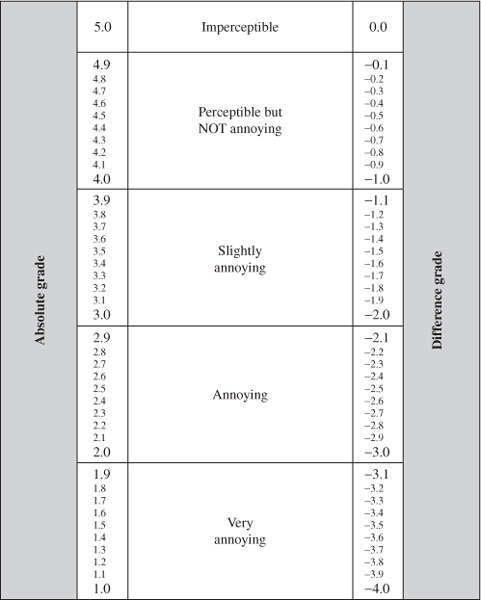
FIGURE 10.24 The subjective quality scale specified by the ITU-R Rec. BS.1116 recommendation. This scale measures small impairments for absolute and differential grading.

The signal selected by the listener as the hidden reference is given a default score of 5.0. Subtracting the score given to the actual hidden reference from the score given to the impaired coded signal yields the subjective difference grade (SDG). For example, original, uncompressed material may receive an averaged score of 4.8 on the scale. If a codec obtains an average score of 4.8, the SDG is 0 and the codec is said to be transparent (subject to statistical analysis). If a codec is transparent, the bit rate may be reduced to determine the coding margin. A lower SDG score (for example, −2.6) assesses how far from transparency a codec is. Numerous statistical analysis techniques can be used. Perhaps 50 listeners are needed for good statistical results. Higher reduction ratios generally score less well. For example, Fig. 10.25 shows the results of a listening test evaluating an MPEG-2 AAC main profile codec at 256 kbps, with five full-bandwidth channels.

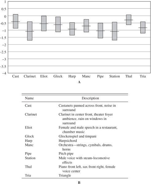
FIGURE 10.25 Results of listening tests for an AAC main profile codec at 256 kbps, five-channel mode showing mean scores and 95% confidence intervals. A. The vertical axis shows the AAC grades minus the reference signal grades. B. This table describes the audio tracks used in this test. (ISO/IEC JTC1/SC29/WG-11 N1420, 1996)

In another double-blind test conducted by Gilbert Soulodre using ITU-R guidelines, the worst-case tracks included a bass clarinet arpeggio, bowed double bass and harpsichord arpeggio (from an EBU SQAM CD), pitch pipe (Dolby recording), Dire Straits (Warner Brothers CD 7599-25264-2 Track 6), and a muted trumpet (University of Miami recording). In this test, when compared against a CD-quality reference, the AAC codec was judged best, followed by PAC, Layer III, AC-3, Layer II, and IT IS codecs, respectively. The highest audio quality was obtained by the AAC codec at 128 kbps and the AC-3 codec at 192 kbps per stereo pair. As expected, each codec performed relatively better at higher bit rates. In comparison to AAC, an increase in bit rate of 32, 64, and 96 kbps per stereo pair was required for PAC, AC-3, and Layer II codecs, respectively, to provide the same audio quality. Other factors such as computational complexity, sensitivity to bit errors, and compatibility to existing systems were not considered in this subjective listening test.

MUSHRA (MUltiple Stimulus with Hidden Reference and Anchors) is an evaluation method used when known impairments exist. This method uses a hidden reference and one or more hidden anchors; an anchor is a stimulus with a known audible limitation. For example, one of the anchors is a lowpass-coded signal. A continuous scale with five divisions is used to grade the stimuli: excellent, good, fair, poor, and bad. MUSHRA is specified in ITU-R BS.1534. Other issues in sound evaluation are described in ITU-T P.800, P.810, and P.830; ITU-R BS.562-3, BS.644-1, BS.1284, BS.1285, and BS.1286, among others.

In addition to listening-test methodology, the ITU-R Recommendation BS.1116-1 standard also describes a reference listening room. The BS.1116-1 specification recommends a floor area of 20 m² to 60 m² for monaural and stereo playback and an area of 30 m² to 70 m² for multichannel playback. For distribution of low-frequency standing waves, the standard recommends that room-dimension ratios meet these three criterion: 1.1(w/h) ≤ (l/h) ≤ 4.5(w/h) − 4; (w/h) < 3; and (l/h) < 3 where l, w, h are the room’s length, width, and height. The 1/3-octave sound pressure level, over a range of 50 Hz to 16,000 Hz, measured at the listening position with pink noise is defined by a standard-response contour. Average room reverberation time is specified to be: 0.25(V/V₀)^1/3 where V is the listening room volume and V₀ is a reference volume of 100 m³. This reverberation time is further specified to be relatively constant in the frequency range of 200 Hz to 4000 Hz, and to follow allowed variations between 63 Hz and 8000 Hz. Early boundary reflections in the range of 1000 Hz to 8000 Hz that arrive at the listening position within 15 ms must be attenuated by at least 10 dB relative to direct sound from the loudspeakers. It is recommended that the background noise level does not exceed ISO noise rating of NR10, with NR15 as a maximum limit.

The IEC 60268-13 specification (originally IEC 268-13) describes a residential-type listening room for loudspeaker evaluation. The specification is similar to the room described in the BS.1116-1 specification. The 60268-13 specification recommends a floor area of 25 m² to 40 m² for monaural and stereo playback and an area of 30 m² to 45 m² for multichannel playback. To spatially distribute low-frequency standing waves in the room, the specification recommends three criterion for room-dimension ratios: (w/h) ≤ (l/h) ≤ 4.5(w/h) − 4; (w/h) < 3; and (l/h) < 3 where l, w, h are the room’s length, width, and height. The reverberation time (measured according to the ISO 3382 standard in 1/3-octave bands with the room unoccupied) is specified to fall within a range of 0.3 to 0.6 seconds in the frequency range of 200 Hz to 4000 Hz. Alternatively, average reverberation time should be 0.4 second and fall within a frequency contour given in the standard. The ambient noise level should not exceed NR15 (20 dBa to 25 dBA).

The EBU 3276 standard specifies a listening room with a floor area greater than 40 m² and a volume less than 300 m³. Room-dimension ratios and reverberation time follow the BS.1116-1 specification. In addition, dimension ratios should differ by more than ±5%. Room response measured as a 1/3-octave response with pink noise follows a standard contour.

Listening Test Statistical Evaluation

As Mark Twain and others have said, “There are three kinds of lies: lies, damned lies, and statistics.” To be meaningful, and not misleading, interpretation of listening test results must be carefully considered. For example, in an ABX test, if a listener correctly identifies the reference in 12 out of 16 trials, has an audible difference been noted? Statistic analysis provides the answer, or at least an interpretation of it. In this case, because the test is a sampling, we define our results in terms of probability. Thus, the larger the sampling, the more reliable the result. A central concern is the significance of the results. If the results are significant, they are due to audible differences. Otherwise they are due to chance. In an ABX test, a correct score 8 of 16 times indicates that the listener has not heard differences; the score could be arrived at by guessing. A score of 12/16 might indicate an audible difference, but could also be due to chance. To fathom this, we can define a null hypothesis H₀ that holds that the result is due to chance, and an alternate hypothesis H₁ that holds it is due to an audible difference. The significance level a is the probability that the score is due to chance. The criterion of significance a is the chosen threshold of a that will be accepted. If a is less than or equal to a then we accept that the probability is high enough to accept the hypothesis that the score is due to an audible difference. The selection of a is arbitrary but a value of 0.05 is often used. Using this formula:

z = (c − 0.5 − np₁)/[np₁(1 − p₁)]^1/2

where z = standard normal deviate

c = number of correct responses

n = sample size

p₁ = proportion of correct responses in a population due to chance alone (p₁ = 0.5 in an ABX test)

We see that with a score of 12/16, z = 1.75. Binomial distribution thus yields a significance level of 0.038. The probability of getting a score as high as 12/16 from chance alone (and not from audible differences) is 3.8%. In other words, there is a 3.8% chance that the listener did not hear a difference. However, since a is less than a (0.038 < 0.05) we conclude that the result is significant and there is an audible difference, at least according to how we have selected our criterion of significance. If a is selected to be 0.01, then the same score of 12/16 is not significant and we would conclude that the score is due to chance.

We can also define parameters that characterize the risk that we are wrong in accepting a hypothesis. A Type 1 error risk (also often noted as a ′) is the risk of rejecting the null hypothesis when it is actually true. Its value is determined by the criterion of significance; if a = 0.05 then we will be wrong 5% of the time in assuming significant results. Type 2 error risk b defines the risk of accepting the null hypothesis when it is false. Type 2 risk is based on the sample size, value of a, the value of a chance score, and effect size or the smallest score that is meaningful. These values can be used to calculate sample size using the formula:

n = {[z₁[p₁ (1 − p₁)]^1/2 + z₂[p₂ (1 − p₂)]^1/2]/(p₂ − p₁)}²

where n = sample size

p₁ = proportion of correct responses in a population due to chance alone (p₁ = 0.5 in an ABX test)

p₂ = effect size: hypothesized proportion of correct responses in a population due to audible differences

z₁ = binomial distribution value corresponding to Type 1 error risk

z₂ = binomial distribution value corresponding to Type 2 error risk

For example, in an ABX test, if Type 1 risk is 0.05, Type 2 risk is 0.10, and effect size is 0.70, then the sample size should be 50 trials. The smaller the sample size, that is, the number of trials, the greater the error risks. For example, if 32 trials are conducted, a = 0.05, and the effect size is 0.70. To achieve a statistically significance result, a score of 22/32 is needed.

Binomial distribution analysis provides good results when a large number of samples are available. Other types of statistical analyses such as signal detection theory can also be applied to ABX testing. Finally, it is worth noting that statistical analysis can appear impressive, but its results cannot validate a test that is inherently flawed. In other words, we should never be blinded by science.

Lossless Data Compression

The principles of lossless data compression are quite different from those of perceptual lossy coding. Whereas perceptual coding operates mainly on data irrelevancy in the signal, data compression operates strictly on redundancy. Lossless compression yields a smaller coded file that can be used to recover the original signal with bit-for-bit accuracy. In other words, although the intermediate stored or transmitted file is smaller, the output file is identical to the input file. There is no change in the bit content, so there is no change in sound quality from coding. This differs from lossy coding where the output file is irrevocably changed in ways that may or may not be audible.

Some lossless codecs such as MLP (Meridian Lossless Packing) are used for stand-alone audio coding. Some lossy codecs such as MP3 use lossless compression methods such as Huffman coding in the encoder’s output stage to further reduce the bit rate after perceptual coding. In either case, instead of using perceptual analysis, lossless compression examines a signal’s entropy.

A newspaper with the headline “Dog Bites Man” might not elicit much attention. However, the headline “Man Bites Dog” might provoke considerable response. The former is commonplace, but the latter rarely happens. From an information standpoint, “Dog Bites Man” contains little information, but “Man Bites Dog” contains a large quantity of information. Generally, the lower the probability of occurrence of an event, the greater the information it contains. Looked at in another way, large amounts of information rarely occur.

The average amount of information occurring over time is called entropy, denoted as H. Looked at in another way, entropy measures an event’s randomness and thus measures how much information is needed to describe it. When each event has the same probability of occurrence, entropy is maximum, and notated as H_max. Usually, entropy is less than this maximum value. When some events occur more often, entropy is lower. Most functions can be viewed in terms of their entropy. For example, the commodities market has high entropy, whereas the municipal bonds market has much lower entropy. Redundancy in a signal is obtained by subtracting from 1 the ratio of actual entropy to maximum entropy: 1 − (H/H_max). Adding redundancy increases the data rate; decreasing redundancy decreases the rate: this is data compression, or lossless coding. An ideal compression system removes redundancy, leaving entropy unaffected; entropy determines the average number of bits needed to convey a digital signal. Further, a data set can be compressed by no more than its entropy value multiplied by the number of elements in the data set.

Entropy Coding

Entropy coding (also known as Huffman coding, variable-length coding, or optimum coding) is a form of lossless coding that is widely used in both audio and video applications. Entropy coding uses probability of occurrence to code a message. For example, a signal can be analyzed and samples that occur most often are assigned the shortest codewords. Samples that occur less frequently are assigned longer codewords. The decoder contains these assignments and reverses the process. The compression is lossless because no information is lost; the process is completely reversible.

The Morse telegraph code is a simple entropy code. The most commonly used character in the English language (e) is assigned the shortest code (.), and less frequently used characters (such as z) are assigned longer codes (- - ..). In practice, telegraph operators further improved transmission efficiency by dropping characters during coding and then replacing them during decoding. The information content remains unchanged. U CN RD THS SNTNCE, thanks to the fact that written English has low entropy; thus its data is readily compressed. Many text and data storage systems use data compression techniques prior to storage on digital media. Similarly, the abbreviations used in text messaging employ the same principles.

Generally, a Huffman code is a noiseless coding method that uses statistical techniques to represent a message with the shortest possible code length. A Huffman code provides coding gain if the symbols to be encoded occur with varying probability. It is an entropy code based on prefixes. To code the most frequent characters with the shortest codewords, the code uses a nonduplicating prefix system so that shorter codewords cannot form the beginning of a longer word. For example, 110 and 11011 cannot both be codewords. The code can thus be uniquely decoded, without loss.

Suppose we wish to transmit information about the arrival status of trains. Given four conditions, on time, late, early, and train wreck, we could use a fixed 2-bit codeword, assigning 00, 01, 10, and 11, respectively. However, a Huffman code considers the frequency of occurrence of source words. We observe that the probability is 0.5 that the train is on time, 0.35 that it is late, 0.125 that it is early, and 0.025 that it has wrecked. These probabilities are used to create a tree structure, with each node being the sum of its inputs, as shown in Fig. 10.26. Moreover, each branch is assigned a 0 or 1 value; the choice is arbitrary but must be consistent. A unique Huffman code is derived by following the tree from the 1.0 probability branch, back to each source word. For example, the code for early arrival is 110. In this way, a Huffman code is created so that the most probable status is coded with the shortest codeword and the less probable are coded with longer codewords. There is a reduction in the number of bits needed to indicate on-time arrival, even though there is an increase in the number of bits needed for two other statuses. Also note that prefixes are not repeated in the codewords.

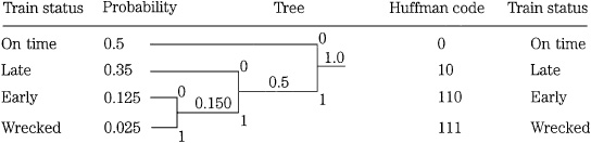
FIGURE 10.26 A Huffman code is based on a nonduplicating prefix, assigning the shorter codewords to the more frequently occurring events. If trains were usually on time, the code in this example would be particularly efficient.

The success of the code is gauged by calculating its average code length; it is the summation of each codeword length multiplied by its frequency of occurrence. In this example, the 1-bit word has a probability of 0.5, the 2-bit words have a probability of 0.35, and the 3-bit words have a combined probability of 0.15; thus the average code length is 1(0.5) + 2(0.35) + 3(0.15) = 1.65 bits. This compares favorably with the 2-bit fixed code, and approaches the entropy of the message. A Huffman code is suited for some messages, but only when the frequency of occurrence is known beforehand. If the relative frequency of occurrence of the source words is approximately equal, the code is not efficient. If an infrequent source word’s probability approaches 1 (becomes frequent), the code will generate coded messages longer than the original. To overcome this, some coding systems use adaptive measures that modify the compression algorithm for more optimal operation. The Huffman code is optimal when all symbols have a probability that is an integral power of one-half.

Run-length coding also provides data compression, and is optimal for highly frequent samples. When a data value is repeated over time, it can be coded with a special code that indicates the start and stop of the string. For example, the message 6666 6666 might be coded as 86. This coding is efficient; run-length coding is used in fax machines, for example, and explains why blank sections of a page are transmitted more quickly than densely written sections. Although Huffman and run-length codes are not directly efficient for music coding by themselves, they are used for compression within some lossless and lossy algorithms.

Audio Data Compression

Perceptual lossy coding can provide a considerable reduction in bit rates. However, whether audible or not, the signal is degraded. With lossless data compression, the signal is delivered with bit-for-bit accuracy. However, the decrease in bit rate is more modest. Generally, compression ratios of 1.5:1 to 3.5:1 are possible, depending on the complexity of the data itself. Also, lossless compression algorithms may require greater processing complexity with the attendant coding delay.

Every audio signal contains information. A rare audio sample contains considerable information; a frequently occurring sample has much less. The former is hard to predict while the latter is readily predictable. Similarly, a tonal (sinusoidal) sound has considerable redundancy whereas a nontonal (noise-like) signal has little redundancy. For example, a quasi-periodic violin tone would differ from an aperiodic cymbal crash. Further, the probability of a certain sample occurring depends on its neighboring samples. Generally, a sample is likely to be close in value to the previous sample. For example, this is true of a low-frequency signal. A predictive coder uses previous sample values to predict the current value. The error in the prediction (difference between the actual and predicted values) is transmitted. The decoder forms the same predicted value and adds the error value to form the correct value.

To achieve its goal, data compression inputs a PCM signal and applies processing to more efficiently pack the data content prior to storage or transmission. The efficiency of the packing depends greatly on the content of the signal itself. Specifically, signals with greater redundancy in their PCM coding will allow a higher level of compression. For that reason, a system allowing a variable output bit rate will yield greater efficiency than one with a fixed bit rate. On the other hand, any compression method must observe a system’s maximum bit rate and ensure that the threshold is never exceeded even during low-redundancy (hard to compress) passages.

PCM coding at a 20-bit resolution, for example, always results in words that are 20 bits long. A lossless compression algorithm scrutinizes the words for redundancy and then reformats the words to shorter lengths. On decompression, a reverse process restores the original words. Peter Craven and Michael Gerzon suggest the example of a 20-bit word length file representing an undithered 4-kHz sine wave at −50 dB below peak level, sampled at 48 kHz. Moreover, a block of 12 samples is considered, as shown in Table 10.4. The file size is 240 bits. Observation shows that in each sample the four LSBs (least significant bits) are zero; an encoder could document that only the 16 MSBs (most significant bits) will be transmitted or stored. This is easily accomplished by right-justifying the data and then coding the shift count. Furthermore, the 9 MSBs in each sample of this low-level signal are all 1s or 0s; the encoder can simply code 1 of the 9 bits and use it to convey the other missing bits. With these measures, because of the signal’s limited dynamic range and resolution, the 20-bit words are conveyed as 8-bit words, resulting in a 60% decrease in data. Note that if the signal were dithered, the dither bit(s) would be conveyed with bit-accuracy by a lossless coder, reducing data efficiency.

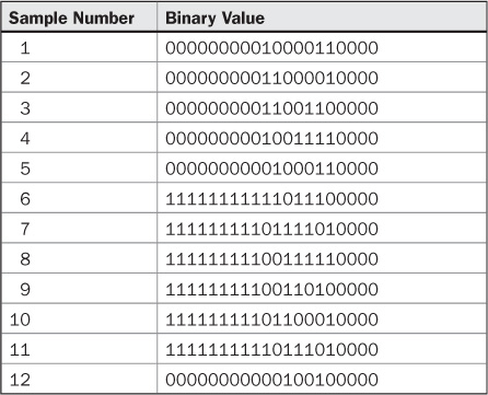
TABLE 10.4 Twelve samples taken from a 20-bit audio file, showing limited dynamic range and resolution. In this case, simple data compression techniques can be applied to achieve a 60% decrease in file size. (Craven and Gerzon, 1996)

In practice, a block size of about 500 samples (or 10 ms) may be used, with descriptive information placed in a header file for each block. The block length may vary depending on signal conditions. Generally, because transients will stimulate higher MSBs, longer blocks cannot compress short periods of silence in the block. Shorter blocks will have relatively greater overhead in their headers. Such simple scrutiny may be successful for music with soft passages, but not successful for loud, highly compressed music. Moreover, the peak data rate will not be compressed in either case. In some cases, a data block might contain a few audio peaks. Relatively few high-amplitude samples would require long word lengths, while all the other samples would have short word lengths. Huffman coding (perhaps using a lookup table) can be used to overcome this. The common low-amplitude samples would be coded with short codewords, while the less common high-amplitude samples would be coded with longer codewords. To further improve performance, multiple codeword lookup tables can be established and selected based on the distribution of values in the current block. Audio waveforms tend to follow amplitude statistics that are Laplacian, and appropriate Huffman tables can reduce the bit rate by about 1.5-bit/sample/channel compared to a simple word-length reduction scheme.

A predictive strategy can yield greater coding efficiency. In the previous example, the 16-bit numbers have decimal values of +67, +97, +102, +79, +35, −18, −67, −97, −102, −79, −35, and +18. The differences between successive samples are +30, +5, −23, −44, −53, −49, −30, −5, +23, +44, and +53. A coder could transmit the first value of +67 and then the subsequent differences between samples; because the differences are smaller than the sample values themselves, shorter word lengths (7 bits instead of 8) are needed. This coding can be achieved with a simple predictive encode-decode strategy as shown in Fig. 10.27 where the symbol z⁻¹ denotes a one-sample delay. If the value +67 has been previously entered, and the next input value is +97, the previous sample value of +67 is used as the predicted value of the current sample, the prediction error becomes +30, which is transmitted. The decoder accepts the value of +30 and adds it to the previous value of +67 to reproduce the current value of +97.

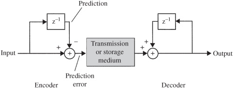
FIGURE 10.27 A first-order predictive encode/decode process conveys differences between successive samples. This improves coding efficiency because the differences are smaller than the values themselves. (Craven and Gerzon, 1996)

The goal of a prediction coder is to predict the next sample as accurately as possible, and thus minimize the number of bits needed to transmit the prediction error. To achieve this, the frequency response of the encoder should be the inverse of the spectrum of the input signal, yielding a difference signal with a flat or white spectrum. To provide greater efficiency, the one-sample delay element in the predictor coder can be replaced by more advanced general prediction filters. The coder with a one-sample delay is a digital differentiator with a transfer function of (1 − z⁻¹). An nth order predictor yields a transfer function of (1 − z⁻¹)ⁿ, where n = 0 transmits the original value, n = 1 transmits the difference between successive samples, n = 2 transmits the difference of the difference, and so on. Each higher-order integer coefficient produces an upward filter slope of 6, 12, and 18 dB/octave. Analysis shows that n = 4 may be optimal, yielding a maximum difference of 10. However, the high-frequency content in audio signals limits the order of the predictor. The high-frequency component of the quantization noise is increased by higher-order predictors; thus a value of n = 3 is probably the limit for audio signals. But if the signal had mainly high-frequency content (such as from noise shaping), even an n = 1 value could increase the coded data rate. Thus, a coder must dynamically monitor the signal content and select a predictive strategy and filter order that is most suitable, including the option of bypassing its own coding, to minimize the output bit rate. For example, an autocorrelation method using the Levinson–Durbin algorithm could be used to adapt the predictor’s order, to yield the lowest total bit rate.

A coder must also consider the effect of data errors. Because of the recirculation, an error in a transmitted sample would propagate through a block and possibly increase, even causing the decoder to lose synchronization with the encoder. To prevent artifacts, audible or otherwise, an encoder must sense uncorrected errors and mute its output. In many applications, while overall reduction in bit rate is important, limitation of peak bit rate may be even more vital. An audio signal such as a cymbal crash, with high energy at high frequencies, may allow only slight reduction (perhaps 1 or 2 bits/sample/channel). Higher sampling frequencies will allow greater overall reduction and peak reduction because of the relatively little energy at the higher portion of the band. To further ensure peak limits, a buffer could be used. Still, the peak limit could be exceeded with some kinds of music, necessitating the shortening of word length or other processing.

The simple integer coefficient predictors described above provide upward slopes that are not always a good (inverse) match for the spectra of real audio signals. The spectrum of the difference signal is thus nonflat, requiring more bits for coding. Every 6-dB reduction in the level of the transmitted signal reduces its bit rate by 1 bit/sample. More successful coding can be achieved with more sophisticated prediction filters using, for example, noninteger-coefficient filters in the prediction loop. The transmitted signal must be quantized to an integer number of LSB steps to achieve a fixed bit rate. However, with noninteger coefficients, the output has a fractional value of LSBs. To quantize the prediction signal, the architecture shown in Fig. 10.28 may be employed. The decoder restores the original signal values by simply quantizing the output.

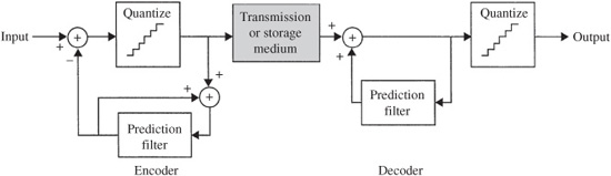
FIGURE 10.28 Noninteger-coefficient filters can be used in a prediction encoder/decoder. The prediction signal is quantized to an integer number of LSB steps. (Craven and Gerzon, 1996)

Different filters can be used to create a variety of equalization curves for the prediction error signal, to match different signal spectral characteristics. Different 3rd-order IIR filters, when applied to different signal conditions, may provide bit-rate reduction ranging from 2 to 4 bits, even in cases where the bit rate would be increased with simple integer predictors. Higher-order filters increase the amount of overhead data such as state variables that must be transmitted with each block to the decoder; this argues for lower-order filters. It can also be argued that IIR filters are more appropriate than FIR filters because they can more easily achieve the variations found in music spectra. On the other hand, to preserve bit accuracy, it is vital that the filter computations in any decoder match those in any encoder. Any rounding errors, for example, could affect bit accuracy. In that respect, because IIR computation is more sensitive to rounding errors, the use of IIR predictor filters demands greater care.

Because most music spectral content continually varies, filter selection must be re-evaluated for each new block. Using some means, the signal’s spectral content must be analyzed, and the most appropriate filter employed, by either creating a new filter characteristic or selecting one from a library of existing possibilities. Information identifying the encoding filter must be conveyed to the decoder, increasing the overhead bit rate. Clearly, processing complexity and data overhead must be weighed against coding efficiency.

As noted, lossless compression is effective at very high sampling frequencies in which the audio content at the upper frequency ranges of the audio band is low. Bit accuracy across the wide audio band is ensured, but very high-frequency information comprising only dither and quantization noise can be more efficiently coded. Craven and Gerzon estimate that whereas increasing the sampling rate of an unpacked file from 64 kHz to 96 kHz would increase the bit rate by 50%, a packed file would increase the bit rate by only 15%. Moreover, low-frequency effects channels do not require special handling; the packing will ensure a low bit rate for its low-frequency content. Very generally, at a given sampling frequency, the bit-rate reduction achieved is proportional to the input word length and is greater for low-precision signals. For example, if the average bit reduction is 9 bits/sample/channel, then a 16-bit PCM signal is coded as 7 bits (56% reduction), a 20-bit signal as 11 bits (45% reduction), and a 24-bit signal as 15 bits (37.5% reduction). Very generally, each additional bit of precision in the input signal adds a bit to the word length of the packed signal.

At the encoder’s output, the difference signal data can be Huffman-coded and transmitted as main data along with overhead information. While it would be possible to hardwire filter coefficients into the encoder and decoder, it may be more expedient to explicitly transmit filter coefficients along with the data. In this way, improvements can be made in filter selection in the encoder, while retaining compatibility with existing decoders.

As with lossy codecs, lossless codecs can take advantage of interchannel correlations in stereo and multichannel recordings. For example, a codec might code the left channel, and frame-adaptively code either the right channel or the difference between the right and left channels, depending on which yields the highest coding gain. More efficiently, stereo prediction methods use previous samples from both channels to optimize the prediction.

Because no psychoacoustic principles such as masking are used in lossless coding, practical development of transparent codecs is relatively much simpler. For example, subjective testing is not needed. Transparency is inherent in the lossless codec. However, as with any digital-processing system, other aspects such as timing and jitter must be carefully engineered.