CHAPTER
FORTY-FIVE
CREDIT-RISK MODELING

TIM BACKSHALL

Chief Credit Derivatives Strategist
Credit Derivatives Research Ltd.

KAY GIESECKE, PH.D.

Assistant Professor of Management Science and Engineering
Stanford University

LISA GOLDBERG, PH.D.

Executive Director of Research
MSCI and
Adjunct Professor of Statistics
University of California at Berkeley

Since the turn of the century, we have seen many theoretical developments in the field of credit-risk research. In view of the large-scale changes in market conditions, the entry of more sophisticated market participants, and the increase in complexity of investable assets, most of the research has focused on pricing of corporate debts. But many of these models have failed to describe real-world phenomena such as credit-spreads realistically. This practitioner-oriented chapter attempts to describe the history and future of modeling credit-risk and valuation of credit-risky assets.

Credit-risk is the distribution of financial losses owing to unexpected changes in the credit quality of the counterparty in a financial agreement. Examples range from agency downgrades to failure to service debt to liquidation. Credit-risk pervades virtually all financial transactions. The distribution of credit losses is complex. At its center is the probability of default, by which we mean any type of failure to honor a financial agreement. To estimate the probability of default, we need to specify

• A model of investor uncertainty

• A model of the available information and its evolution over time

• A model definition of the default event.

However, default probabilities alone are not sufficient to price credit-sensitive securities. We need, in addition,

• A model for the risk-free interest rate

• A model of recovery on default

• A model of the premium investors require as compensation for bearing systematic credit-risk

The credit premium maps actual default probabilities to market-implied probabilities that are embedded in market prices. To price securities that are sensitive to the credit-risk of multiple issuers and to measure aggregated portfolio credit-risk, we also need to specify

• A model that links defaults of different entities

There are three main quantitative approaches to analyzing credit. In the structural approach, we make explicit assumptions about the dynamics of a firm’s assets, its capital structure, and its debt and share holders. A firm defaults if its assets are insufficient according to some measure. In this situation, a corporate liability can be characterized as an option on the firm’s assets. The reduced-form approach is silent about why a firm defaults. Instead, the dynamics of default are given exogenously through a default rate, or intensity. In this approach, prices of credit-sensitive securities can be calculated as if they were default-free using an interest rate that is the risk-free rate adjusted by the intensity. The incomplete-information approach combines the structural and reduced-form models. While avoiding their difficulties, it picks the best features of both approaches: the economic and intuitive appeal of the structural approach and the tractability and empirical fit of the reduced-form approach.

In this chapter we review the three approaches in the context of the multiple facets of credit modeling that were just mentioned. Our goal is to provide a concise overview and a guide to the large and growing literature on credit-risk.¹

STRUCTURAL CREDIT MODELS

The basis of the structural approach, which goes back to Black and Scholes² and Merton,³ is that corporate liabilities are contingent claims on the assets of a firm. The market value of the firm is the fundamental source of uncertainty driving credit-risk.

Classical Approach

Consider a firm with market value V, which represents the expected discounted future cash-flows of the firm. The firm is financed by equity and a zero-coupon bond with face value K and maturity date T. The firm’s contractual obligation is to repay the amount K to the bond investors at time T. Debt covenants grant bond investors absolute priority: if the firm cannot fulfill its payment obligation, then bondholders immediately will take over the firm.

Exhibit 45–1 shows several possible paths of firm value. Default occurs if the firm value at maturity is less than the face value of the debt K. The particular path the firm value has taken does not matter here; only the firm value at T is important. The probability of default therefore is equal to the probability that firm value is below debt face value at maturity. To calculate this probability, we make assumptions about the distribution of firm value at debt maturity. The standard assumption is that firm value is log-normally distributed. The probability of default then is given as the area under the log-normal firm value density between 0 and face value, as shown in the graph. This probability can be calculated explicitly in terms of K, the current firm value V(0), the volatility of firm value, the growth rate of firm value and T.

EXHIBIT 45–1
Default Interpretation in the Classical Approach

Assuming that the firm can neither repurchase shares nor issue new senior debt, the payoffs to the firm’s liabilities at debt maturity T are as summarized in Exhibit 45–2. If the asset value V(T) exceeds or equals the face value K of the bonds, the bondholders will receive their promised payment K, and the shareholders will get the remaining V(T) – K. However, if the value of assets V(T) is less than K, the ownership of the firm will be transferred to the bondholders, who lose the amount K – V(T). Equity is worthless because of limited liability.

EXHIBIT 45–2
Payoffs at Maturity in the Classical Approach

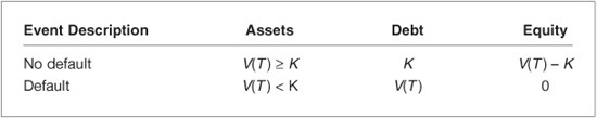
Summarizing, the value of the bond is equivalent to that of a portfolio composed of a default-free loan with face value K maturing at time T and a short European put position on the assets of the firm with strike K and maturity T. The value of the equity is equivalent to the payoff of a European call option on the assets of the firm with strike K and maturity T. Pricing equity and credit-risky debt thus reduces to pricing European options.

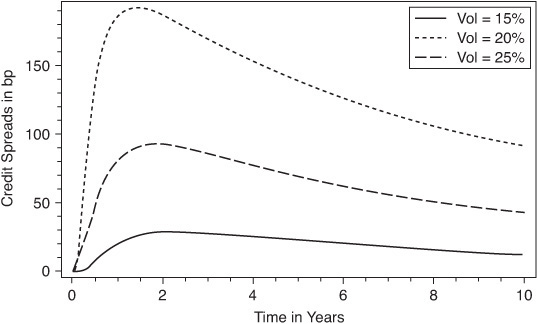
The credit-spread is the difference between the yield on a defaultable bond and the yield on an otherwise equivalent default-free zero bond. It gives the excess return demanded by bond investors to bear the potential default losses. The credit-spread is a function of maturity T, asset volatility (the firm’s business risk), the initial leverage ratio K/V(0), and risk-free rates.

Letting initial leverage be 80% and risk-free rates be 6%, in Exhibit 45–3 we plot the model term structure of credit-spreads for varying asset volatilities. We see clearly that as asset volatility (business risk) rises, then so does the spread required by the market to compensate for the risk of default. Other noticeable traits of this graph are the rapid fall to zero spreads at short maturities and the more pronounced hump-shaped curve as volatility rises higher.

EXHIBIT 45–3
Term Structure of Credit-Spreads, Varying Asset Volatility, in the Classical Approach

First-Passage Approach

In the classical approach, firm value can dwindle to almost nothing without triggering default. This is unfavorable to bondholders, as noted by Black and Cox.⁴ Bond indenture provisions often include safety covenants that give bond investors the right to reorganize a firm if its value falls below a given barrier.

First-passage time models generalize the classical model such that a default can occur not only at maturity of the debt contract but also at any point of time. They assume that default happens if the firm value V hits a specified default barrier D. The default barrier in general can be a stochastic process, as is the firm value. For tractability reasons, however, one often works with a simple time-dependent, nonstochastic barrier specification, or just a constant barrier.

Suppose that the default barrier D is a constant between zero and the initial firm value—this is reasonable because we would expect liabilities to be nonnegative and less than current assets. Then the default time is more realistically defined as when the value of the firm crosses below the default barrier. In other words, firms can default at times other than debt maturity. This relaxation of the European nature of the default event in the classical approach provides some more realistic behavior.

Exhibit 45–4 shows several possible paths of firm value and a constant default barrier D. Suppose for the moment that D is equal to the face value of the firm’s debt. Default occurs if the firm value falls, at any time before the horizon T, below the default barrier. As shown, different firm-value paths correspond to different default times. Unlike the classical model discussed earlier, here the entire path the firm value follows is relevant. Firm-value paths that imply survival in the classical approach can imply default in the first-passage approach. Therefore, the first-passage approach implies higher probabilities of default than the classical approach.

EXHIBIT 45–4
Default in the First-Passage Approach

The probability of default is given by the probability that the minimum firm value at the horizon M(T) is lower than the barrier D. In order to calculate this probability, we make an assumption about the distribution of future firm values, as in the classical approach. This determines also the distribution of the minimum firm value at the horizon. With log-normal firm values, this distribution is inverse gaussian. The default probability is given as the area under the inverse gaussian density curve between 0 and the default barrier D.

We consider the payoff to investors in the firm’s liabilities. For simplicity, we assume that the default barrier is equal to the face value of firm debt. If the firm value never fell below the barrier over the term of the bond, then bond investors receive the bond’s face value K and equity investors would receive the remaining V(T) – K. However, if the firm falls below the barrier at some point during the bond’s term, then the firm defaults. In this case the firm stops operating, bond investors take over its remaining assets, and equity investors receive nothing.

Therefore, the equity position is equivalent to that of a down-and-out call on firm assets with strike equal to the face value of the debt, barrier level equal to the default barrier, and maturity equal to debt maturity. The value of the debt is given as the difference between firm value and equity value. Pricing equity and credit-risky debt thus reduces to pricing European barrier options.

We consider the credit-spread implied by a first-passage model in Exhibit 45–5. We assume that the default barrier is constant and equal to the face value of the bonds. We set leverage equal to 60% and risk-free rates to 6%, as in Exhibit 45–3. We assume that in the event of default, bond investors recover a fraction of 50% of their initial investment.

EXHIBIT 45–5
Term Structure of Credit-Spreads, Varying Asset Volatility, in the First-Passage Model

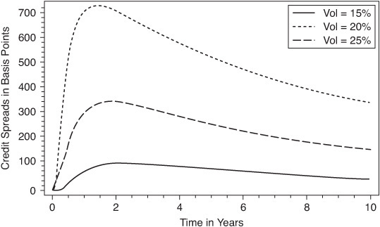
With increasing maturity T, the spread asymptotically approaches zero. This is at odds with empirical observation; for many firms, spreads tend to increase with increasing maturity, reflecting the fact that uncertainty is greater in the distant future than in the near term. This discrepancy follows from two model properties: the firm value grows at a positive (risk-free) rate, and the capital structure is constant and assumed known with certainty. We can address this issue by assuming that the total debt grows at a positive rate or that firms maintain some target leverage ratio as in Collin-Dufresne and Goldstein.⁵ A critical insight from this plot is that the level of spreads in the first-passage model is much higher and much more realistic than in the classical model. This is due to the fact that default probabilities are higher in the first-passage approach, as we discussed earlier.

Dependent Defaults

Credit-spreads of different issuers are correlated through time. Two patterns are found in time series of spreads. The first is that spreads vary smoothly with general macroeconomic factors in a correlated fashion. This means that firms share a common dependence on the economic environment, which results in cyclic correlation between defaults. The second relates to the jumps in spreads: we observe that these are often common to several firms or even entire markets. This suggests that the sudden large variation in the credit-risk of one issuer, which causes a spread jump in the first place, can propagate to other issuers as well. The rationale is that economic distress is contagious and propagates from firm to firm. A typical channel for these effects are borrowing and lending chains. Here the financial health of a firm also depends on the status of other firms as well.

We want to incorporate these two default correlation mechanisms into the structural approach to credit. To introduce cyclic correlation, it is natural to assume that firm values of several firms are correlated through time. This corresponds to common factors driving asset returns. We consider the simplest case with two firms whose firm values are log normal. Our definition of default follows the classical approach.

Exhibit 45–6 illustrates the situation. The axes show the marginal asset return distributions of the two firms. Individual asset returns are normally distributed, hence the bell shape. Individual returns are modeled through a linear factor model, which represents systematic and firm-specific risk. Systematic risk is modeled by a common latent factor X, which drives the systematic variation in the asset returns of both firms. The sensitivity of a firm’s return to this common factor controls the asset correlation across firms. This asset correlation drives the default correlation between firms.

EXHIBIT 45–6
Illustrative Example of Structural-Based Joint Default Modeling

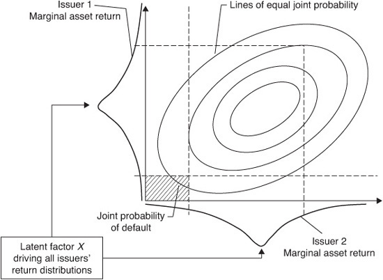
The elliptical shapes represent lines of equal joint asset value probability. The shaded area on the bottom left illustrates the joint default probability, as defined by the area under which issuer 1’s asset value is below its default barrier and issuer 2 is below its default barrier.

Asset correlation captures the dependence of firms on common economic factors in a natural way. Modeling default contagion effects is much more difficult. A straightforward idea is to consider a jump-diffusion model for firm value. We would stipulate that a downward jump in the value of a given firm triggers subsequent jumps in the firm values of other firms with some probability. This would correspond to the propagation of economic distress. This approach is difficult, however, because of the lack of closed-form results on the joint distribution of firms’ historical asset lows. This is what we need to calculate the probability of joint default.

A more successful attempt is to introduce interaction effects through the default barriers D_i. Suppose that the barrier is random and depends on the firm’s liquidity state, which, in turn, depends on the default status of the firm’s counter-parties. If a firm’s liquidity reserves are stressed owing to a payment default of a counterparty, it finances the loss by issuing more debt. This increases the default, barrier: the firm is now more likely to default, all else being equal. With no counterparty defaults the default barrier remains unaffected. This model allows a closed-form approximation of the credit portfolio loss distribution.

Credit Premium

Issuers of credit-sensitive securities share a common dependence on the economic environment. It follows that aggregated credit-risk cannot be diversified away. This undiversifiable or systematic risk commands a premium, which compensates risk-averse investors for assuming credit-risk.

The credit premium is empirically well documented. Its importance relates to the uses of a quantitative credit model. As a default probability forecasting tool, a credit model must reflect the historical default experience. As a tool for pricing credit-sensitive securities, it must fit observed market prices. To make use of both market data and historical default data in the calibration and application of a credit model, we need to understand the relationship between actual defaults and defaultable security prices.

Here the risk premium comes into play: it maps the actual likelihood of default p(T) into the market-implied likelihood of default q(T) that is embedded in security prices.

We examine the difference between the two using a simple example in Exhibit 45–7. We consider a one-period market with two securities, a risk-free bond paying 10 and trading at 10 (risk-free rates are zero) and a defaultable bond trading at 5 that pays 20 in case of no default and zero in case the issuer defaults by the end of the trading period.

EXHIBIT 45–7
Real-World versus Market-Implied Probability of Default

Suppose that the actual probability of default is p = 0.5 (50%, or a coin flip). This is, however, not the probability the market uses for pricing the bond: it would lead to a price of p.20 + (1 – p).0 = 10, which is double the price at which the bonds are actually trading. At this price, risk-averse investors would rather put their money into the risk-free bond that costs 10 as well, unless they get a discount as compensation for the default risk. The market requires a discount of 5, and the corresponding price reflects the market-implied probability of default q, which satisfies 5 = (1 – q).20. This yields q = 0.75 (75% probability of default), which is bigger than the actual probability of default p = 0.5.

To account for risk aversion in calculating the expected payoff of the defaultable bond, the market puts more weight on the unfavorable states of the world in which the firm defaults. In the structural credit models with firm value dynamics as described previously and constant risk-free rates, the situation is only a little more complicated.

In the absence of arbitrage opportunities, the credit-risk premium α is uniquely determined through market prices of credit-sensitive securities such as equity or debt and is measured as the excess return on firm assets over the risk-free return per unit of firm risk measured in terms of asset volatility. If the market is risk-averse, then α is positive: investors in credit-risky firm assets require a return that is higher than the risk-free return. The excess return on any credit-sensitive security is given by its volatility times α.

Calibration

The calibration of a quantitative credit model is closely related to its use. To price single-name credit-sensitive securities using a structural model, we need to calibrate the risk-free rate, the asset volatility, the asset value, the face value of the debt, the default barrier, and the maturity of the debt. The default barrier is relevant only in the first-passage approach. To use the model to forecast actual default probabilities, we need to calibrate additionally the growth rate of firm assets or, equivalently, the credit-risk premium α. In a multiple-firm setting we need to estimate asset correlations in addition to the single-name parameters.

Firm values are not observable. The goal is to estimate the parameters of the firm-value process based on equity prices, which can be observed for public firms. Risk-free interest rates can be estimated from default-free Treasury bond prices via standard procedures. We bypass estimation of face value and maturity of firm debt from balance-sheet data, which is nontrivial given the complex capital structure of firms. In practice, these parameters often are fixed ad hoc, as some average of short- and long-term debt, for example. We introduce a more reasonable solution to this problem later.

We consider the classical approach, as briefly discussed earlier. Given equity prices and equity volatilities, Jones, Mason, and Rosenfeld and many others suggest to back out asset values and asset volatilities by numerically solving a system of two equations.⁶ The first equation relates the equity price to asset value, time, and asset volatility and follows from the Black-Scholes pricing function for a European call with strike K and maturity T. The second equation relates the equity price to asset and equity volatility, the delta of equity, and asset value. This relation is obtained from applying Ito’s formula to the first equation.

We can use these two equations to “translate” a time series of equity values into a time series of asset values and volatilities. As for the equity volatility, we can use the empirical standard deviation of equity returns or a true forecasting model such as Barra Equity Risk models. Given a time series of asset returns, the empirical growth rate yields an estimate of the market price of credit-risk. The estimate of the firm growth rate, however, is very poor: it is based on two asset-return observations only.

Further, given the asset-return time series of several firms, asset correlation can be estimated. Alternatively, we can introduce a linear-factor model for normally distributed asset returns that expresses the idea that firms share a common dependence on general economic factors. This is similar to the idea we discussed earlier.

Can We Predict the Future?

To a certain extent, users of structural models implicitly assume that they can. In structural models, firm value is the single source of uncertainty that drives credit-risk. Investors observe the distance of default as it evolves over time. If the firm value has no jumps, this implies that the default event is not a total surprise. There are “predefault events” that announce the default of a firm. In the first-passage approach, we can think of a predefault event as the first time assets fall dangerously close to the default barrier (see Exhibit 45–8).

EXHIBIT 45–8
Announcing the Default Timing by a Sequence of “Predefault” Events in the First-Passage Approach

This has significant implications for the fitting of structural models to market prices. First, since default can be anticipated, the model price of a credit-sensitive security converges continuously to its recovery value. Second, the model credit-spread tends to zero with time to maturity going to zero.⁷ Quite telling in this regard are the credit-spreads implied by the classical and first-passage approaches (see Exhibits 45–3 and 45–5). Both properties are at odds with intuition and market reality. Market prices do exhibit surprise downward jumps on default. Even for very short maturities in the range of weeks, market credit-spreads remain positive. This indicates that investors do have substantive short-term uncertainty about defaults, in contrast to the predictions of the structural models.

REDUCED-FORM CREDIT MODELS

Reduced-form models were developed in the 1990s.⁸ Here we assume that default occurs without warning. This means that investors face short-term credit-risk, which is absent from the structural models discussed previously. This is a desirable model property because it allows us to fit the model to market credit-spreads.

Default Intensity

The rate at which default occurs is called the default intensity, and we denote it by λ. We can think of the intensity at time t as the conditional probability that default will happen immediately, given that the firm has escaped default by t. As such, it describes the short-term credit-risk investors face.

The intensity is the central ingredient of all reduced-form models. It is modeled as a (nonnegative) stochastic process under the market-implied probability. The time evolution of the intensity reflects changes in the instantaneous default probability of a firm. The intensity model is calibrated from market prices of credit-sensitive securities issued by the firm. There is a one-to-one relation between the intensity and the corresponding default probabilities.

We give two simple but useful specifications for the intensity and the corresponding default probabilities.

• Example 1. Suppose that λ is a constant. Then default is a Poisson arrival, and the default time is exponential with parameter λ. The default probability thus is given by q(T) = 1 – exp(λT).

• Example 2. Suppose that λ = λ(t) is a deterministic function of time t. Then default is an inhomogeneous Poisson arrival. A simple but useful parameterization that is frequently used is the assumption that K(t) is stepwise defined over finite periods across the spread curve—these stepwise constants can be calibrated easily from market data.

These examples constitute only a small sample of possible parameterizations of the default intensity. There are many more choices, often borrowed from the classical term-structure models based on the short-term interest rate. This is motivated by the close analogy of defaultable term-structure models and classical, nondefaultable term-structure models to which we turn next.

Valuation

The description of the default dynamics through the market-implied default intensity λ leads to tractable valuation formulas. Below we describe several different specifications of these formulas corresponding to different units for the value recovered by investors at default.

We consider a zero-coupon bond paying 1 at maturity T if there is no default and a fraction 0 < R < 1 of an equivalent (face value 1, maturity T) but default-free bond at default if default occurs before maturity T. This recovery specification is often called equivalent recovery. Given the market-implied probability of default q(T), and assuming that R is a constant, the present value of the bond can be written as exp(–rT) – exp(–rT)(1 – R)q(T). Here, r is the constant risk-free rate of interest. Thus the value of the bond is the value of an otherwise equivalent risk-free bond minus the present value of the default loss (1 – R). If the intensity is constant (Example 1) and recovery is zero, we obtain for the bond price today exp[ – (r+λ) T]. This means that the value of the defaultable bond is calculated as if the bond were risk-free by using a default-adjusted discount rate. The new discount rate is the sum of the risk-free rate r and the intensity λ. This parallel between pricing formulas for defaultable bonds and otherwise equivalent default-free bonds is one of the best features of reduced-form models.

An alternative recovery model is called fractional recovery of predefault market value. Here it is assumed that the bond recovers a fraction 0 < R < 1 of the market value of the bond just prior to default. If the recovery rate and the intensity are constant (Example 1 above), we obtain the following convenient formula for the bond price: exp{–[r + λ(1 – R)]T}. This is the value of a zero-recovery defaultable bond when the issuer’s default intensity is “thinned” to λ(1 – R). The intuition behind this is as follows. Suppose that the bond defaults with intensity λ. At default, the bond becomes worthless with probability (1 – R), and its value remains unchanged with probability R. Clearly, the predefault value of the bond is not changed by this way of looking at default. Consequently, for pricing, we can ignore the “harmless” default, which occurs with intensity λR. We then price the bond as if it had zero recovery and a default intensity of λ(1 – R). The fractional-recovery pricing formula is then implied by the formula for equivalent recovery.

The results for the valuation of more complex credit-sensitive securities are analogous, and in the general case, a credit-sensitive security can be valued as if it were not sensitive to credit-risk by using an adjusted rate for discounting payoffs.

We take a closer look at the credit-spreads implied by reduced-form models. In the simple case where recovery is zero and some technical conditions are satisfied, we can show that short-term credit-spreads tend to λ and not zero. This should be contrasted with the structural models, where the spread goes to zero with time to maturity going to zero. In the reduced-form models, the default event is unpredictable; it comes without warning. There is always short-term uncertainty about the default event, for which investors demand a premium. This premium, expressed in terms of yield, is given by the intensity.

The unpredictability of default has another important consequence. In line with empirical observation, the model price of a credit-sensitive security will drop abruptly to its recovery value on default. This is in direct conflict with the structural models considered earlier, in which the price converges to its default contingent value and remains there as equity value drops to zero.

Default Correlation

In the reduced-form approach we can introduce cyclical default correlation by assuming that firms’ default intensities are correlated through time. Similarly to the structural models of correlated default, we can introduce systematic and firm-specific factors that drive the intensities of firms. The sensitivity of a firm with respect to the systematic factors controls the intensity correlation across firms. This intensity correlation drives the dependence between firm defaults. Joint default probabilities can be calculated by observing that the intensity of the first default in a portfolio of names is the sum of the default intensities of the individual issuers in the portfolio.

Reduced-form models provide a flexible framework for modeling the dynamics of multiple-issuer credit-risk. However, calibration of the model to market variables is not trivial because of the scarcity of default data and the need to model a large number of parameters simultaneously. There are also studies that argue that the approach can be problematic for other reasons.

Taking account of contagious default correlation in the reduced-form approach is not an easy exercise. The idea is that there are correlated jumps in firms’ default intensities corresponding to the correlated jumps we observe in credit-spreads. A variant of this assumes that there are marketwide events that can trigger joint defaults.⁹ Another variant assumes that the default intensity of a firm depends explicitly on the default status of related counterparty firms in the market.¹⁰ To avoid running into a circularity problem, one can suppose that only the default of designated “primary” firms has an effect on other “secondary” firms.

While Jarrow and Yu¹¹ focus on the pricing of credit-sensitive securities in the presence of contagion effects, it is difficult to calculate joint default probabilities and portfolio loss distributions within this approach. As Davis and Lo¹² and Giesecke and Weber¹³ show, one can obtain tractable closed-form characterizations of loss distributions at the cost of more restricting assumptions that relate to the homogeneity of firms and the symmetry in their counterparty relations.

Calibration

Reduced-form models typically are formulated directly under the market-implied probability. This suggests that we calibrate directly from market prices of various credit-sensitive securities. One often uses liquid debt prices or credit default swap spreads, although Jarrow argues that equity is a good candidate as well.¹⁴ Depending on the characteristics of the calibration security, it may be necessary to make parametric assumptions about the recovery process as well. With fractional recovery and zero bonds, for example, the problem is to choose the parameters of the adjusted short rate model r + λ(1 – R) such that model bond prices best fit observed market prices.

Here one can either parameterize the adjusted short rate directly or specify the component processes separately. With a separate specification, identification problems may arise because only the product λ(1 – R) enters the pricing formula just described. In general, in the estimation problem one can draw from the experience related to nondefaultable term-structure models given the close analogy to reduced-form defaultable models.¹⁵

INCOMPLETE-INFORMATION CREDIT MODELS

For the purpose of measuring default risk, neither the structural nor the reduced-form model explicitly accounts for the fact that investors rely on information that is imperfect. The framework described in this section addresses this issue directly by giving a common perspective on reduced-form and structural models. This perspective leads to previously unrecognized hybrid models that incorporate the best features of both traditional approaches while avoiding their shortcomings.

Incomplete-information credit models were introduced by several researchers.¹⁶ Giesecke and Goldberg¹⁷ describe a structural reduced-form hybrid default model based on incomplete information. This model, hereafter denoted I², is a first-passage time model: it assumes that a firm defaults when its value falls below a barrier. All first-passage time models require descriptions of both firm value and a default barrier. What distinguishes the I² model from traditional first-passage time models as we described them earlier is that it assumes that investors do not know the default barrier. The importance of modeling uncertainty about the default barrier is highlighted by high-profile scandals at firms such as Enron, Tyco, and WorldCom. In these cases, public information led to poor estimates of the default barrier.

Both the expected default barrier and the uncertainty around it can be calibrated to available information in the I² model. Imagine that a firm is believed to be in good financial health but that a particular analyst thinks otherwise. The analyst can increase the forecasts to line up with her views by raising the expected value of the barrier. She also can adjust the variance of the default barrier to the level of her confidence in reported levels of the firm’s liability.

Other incomplete-information models can be envisioned. We can think of a situation where we cannot observe firm values or receive noisy or lagged firm-value information. Another situation is when we are uncertain about both firm values and the default barrier.

With incomplete information, default becomes a surprise event. It cannot be anticipated any more, as it can in the traditional first-passage models. It follows that investors face short-term credit-risk as in the reduced-form models. With short-term uncertainty, the model prices generated by the incomplete-information models provide an excellent fit to market prices. In particular, model prices are consistent with the jumps in prices observed around the default announcement. Model spreads are consistent with the nonzero short-term spreads observed in the credit markets. Exhibit 45–9 shows the term structure of credit-spreads implied by the I² model, assuming risk-free rates of 6%. Strictly positive short spreads reflect the compensation for the short-term credit-risk that investors face.

EXHIBIT 45–9
Term Structure of Credit-Spreads, Varying Asset Volatility, in the I² Model

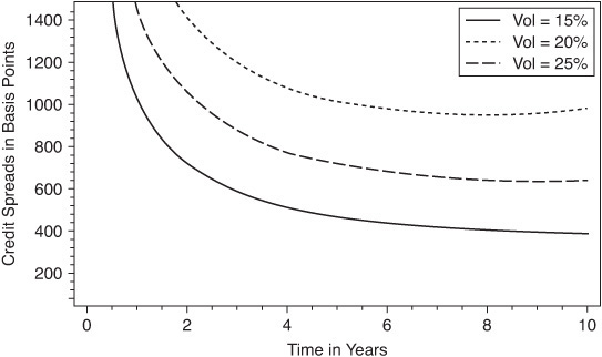
Giesecke and Goldberg calibrate the I² model from market data and further analyze its empirical properties. In particular, the I² model output is compared empirically with a traditional first-passage model. Two main conclusions can be drawn. The I² model reacts more quickly because it takes direct account of the entire history of public information rather than just current values. Furthermore, the I² model predicts positive short spreads for firms in distress. The traditional first-passage model always predicts that short spreads are zero.

Dependent Defaults

Since incomplete-information models are based on the structural approach, we can model cyclical default correlation through firm-value correlation.

Contagious default correlation arises very naturally with incomplete information. Consider the I² model. With defaults of firms arriving over time, we learn about the unobserved default barriers of the surviving firms.¹⁸ This means that we update the distribution we put on a firm’s default barrier with the information we extract from the unanticipated defaults of counterparty firms and reassess firms’ default probabilities. The situation in which we do not directly observe firm values is very similar.¹⁹ In both scenarios, the “contagious” jumps in credit-spreads we observe in credit markets are implied by informational asymmetries.

Credit Premium

The credit-risk premium is the mapping between the actual probability and the market-implied probability. To understand the structure of the premium, we examine the dynamics of firm value and corporate liabilities in the I² model. We argued earlier that thanks to the unpredictability of default, prices of credit-sensitive claims including firm equity and debt drop precipitously at default. Empirical observation shows that equity drops to near zero. This makes sense because equity holders have no stake in the firm after default. The value of the bonds is diminished by bankruptcy costs, which is described by some fractional recovery R.

Consequently, firm value, which is equal to the sum of equity and debt values, also drops at default. This is shown in Exhibit 45–10. Therefore, there are two sources of uncertainty related to firm value:

EXHIBIT 45–10
Firm Value in the Incomplete-Information Model

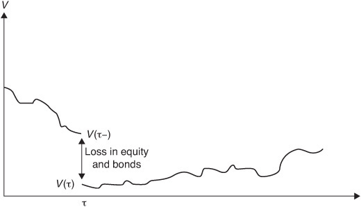
• The first is the diffusive uncertainty.

• The second is the uncertainty associated with the downward jump at default.

Giesecke and Goldberg show that in the I² model the credit-risk premium can be decomposed into two components, which correspond to the two sources of uncertainty:²⁰

• The diffusive risk premium α compensates investors for the diffusive uncertainty in firm value. As in the traditional structural models, it is realized as a change to the drift term in firm-value dynamics.

• The default event risk premium β is not present in the traditional structural models. It compensates investors for the jump uncertainty in firm value and is realized as a change to the default probability. Driessen²¹ empirically confirms that this event risk premium is a significant factor in corporate bond returns.

Giesecke and Goldberg demonstrate that the assumption of no arbitrage is realized in the mathematical relationships among α, β, the recovery rate assumed by the market, and the coefficients of the price processes of traded securities. The price processes depend explicitly on the leverage ratio, so the premia α and β do as well. As Giesecke and Goldberg discuss,²² this violates an important condition for the Modigliani and Miller theorem.²³ The I² model therefore is not consistent with the Modigliani-Miller theorem. It provides a new way to measure the deviation of real markets from the idealized markets in which the Modigliani-Miller theorem holds.

The structure of the incomplete-information risk premium is analogous to the risk premium in reduced-form models considered in El Karoui and Martellini²⁴ and Jarrow, Lando, and Yu.²⁵ The diffusive premium related to the firm-value process corresponds to a premium for diffusive risk in the default intensity process. The event risk premium is analogous to the default event risk premium in intensity-based models. However, in the incomplete-information setting it is defined in the general reduced-form context where an intensity need not exist.

Calibration

There is a lively debate in the literature concerning which data should be used to calibrate credit. Jarrow²⁶ points to a division between structural and reduced-form modelers on this issue. Traditionally, structural models are fit to equity markets and reduced-form models are fit to bond markets. Jarrow argues that the equity and bond data can be used in aggregate to calibrate a credit model, and he gives a recipe for doing this in a reduced-form setting.

Giesecke and Goldberg²⁷ apply reasoning similar to that of Jarrow to calibrate the I² model. The estimation procedure makes use of historical default rates in conjunction with data from equity, bond, and credit default swap markets. Huang and Huang²⁸ give empirical evidence that structural models yield more plausible results if calibrated to both kinds of data. Importantly, the physical and market-implied probabilities are fit simultaneously. The output of the calibration includes estimates of the risk premium, market-implied recovery, model security prices, and physical probabilities of default.

One issue addressed in Giesecke and Goldberg²⁹ is the relationship between model and actual capital structures. In the classical setting, equity is a European option, with strike price and date equal to the face value and maturity of a zero bond. This model fits market data only to the extent that firm debt can be represented adequately as a zero bond. Giesecke and Goldberg make use of the flexibility imparted by incomplete information to give a more realistic picture of equity. Specifically, equity is a down-and-out call with a stochastic strike price. This approach sidesteps the intractable problem of describing a complex capital structure in terms of a single face value and maturity date.

KEY POINTS

• Credit-risk is the distribution of financial losses owing to unexpected changes in the credit quality of the counterparty in a financial agreement.

• Estimating probability of default requires the specification of a (1) model of investor uncertainty, (2) model of the available information and its evolution over time, and (3) model definition of the default event.

• Because default probabilities alone are not sufficient to price credit-sensitive securities, it is necessary to have a (1) model for the risk-free interest rate, (2) model of recovery on default, and (3) model of the premium investors require as compensation for bearing systematic credit-risk.

• The credit premium maps actual default probabilities to market-implied probabilities that are embedded in market prices.

• In order to price securities that are sensitive to the credit-risk of multiple issuers and measure aggregated portfolio credit-risk, a model that links defaults of different entities must be specified.

• The three main quantitative approaches to analyzing credit are the structural approach, the reduce-form approach, and the incomplete-information approach.

• The basis of the structural approach is the Black-Scholes-Merton framework, in which corporate liabilities are contingent claims on the assets of a firm. The market value of the firm is the fundamental source of uncertainty driving credit-risk. The structural approach makes explicit assumptions about the dynamics of a firm’s assets, its capital structure, and its debt and share holders. A firm defaults if its assets are insufficient according to some measure. In this situation, a corporate liability can be characterized as an option on the firm’s assets.

• First-passage time structural models generalize the classical model such that a default can occur not only at maturity of the debt contract, but also at any point of time.

• Credit-spreads of different issuers are correlated through time and must be incorporated into a credit-risk model. Two patterns are found in time series of spreads: (1) spreads vary smoothly with general macroeconomic factors in a correlated fashion, and (2) there are jumps in spreads that are common to several firms or even entire markets.

• Reduced-form models assume that default occurs without warning. That is, this approach is silent about why a firm defaults. Instead, the dynamics of default are given exogenously through a default rate, or intensity. In this approach, prices of credit-sensitive securities can be calculated as if they were default-free using an interest rate that is the risk-free rate adjusted by the intensity. Default intensity is the rate at which defaults occur.

• The incomplete-information approach combines the best features of the structural and reduced-form models while at the same time avoiding the shortcomings of the two models. More specifically, it combines the economic and intuitive appeal of the structural approach and the tractability and empirical fit of the reduced-form approach.