
Useful Facts and Formulas
C.1 Greek Alphabet
| Alpha | A | α |
| Beta | B | β |
| Gamma | γ | |
| Delta | Δ | δ |
| Epsilon | E | ε |
| Zeta | Z | ζ |
| Eta | E | η |
| Theta | Θ | θ |
| Iota | I | ι |
| Kappa | K | κ |
| Lambda | Λ | Λ |
| Mu | M | μ |
| Nu | N | ν |
| Xi | Ξ | ξ |
| Omicron | Π | ο |
| Pi | Π | π |
| Rho | Ρ | Ρ |
| Sigma | Σ | σ |
| Tau | Τ | τ |
| Upsilon | Υ | υ |
| Phi | Φ | φ |
| Chi | Χ | χ |
| Psi | Χ | ψ |
| Omega | Ω | ω |
C.2 Powers of 10 Unit Prefixes
| PREFIX | SYMBOL | MULTIPLYING FACTOR |
| tera | T | × 1012 |
| giga | G | × 109 |
| mega | M | × 106 |
| kilo | K | × 103 |
| centi | c | × 10-2 |
| milli | m | × 10-3 |
| micro | μ | × 10-6 |
| nano | n | × 10-9 |
| pico | p | × 10-12 |
C.3 Linear Functions (y = mx + b)
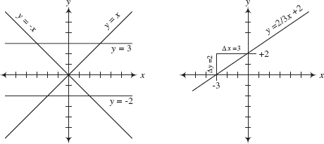
The equation y = mx + b represents the equation of a line. The slope of the line (Δy/Δx) is equal to m, while the vertical shift, or point where the line crosses the y axis, is equal to b.
FIGURE C.1
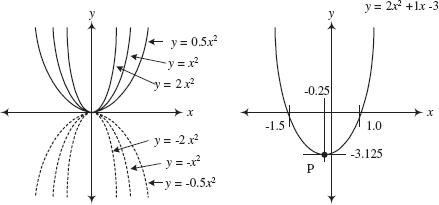
The equation y = ax2 + bx + c traces out a parabola in the xy plane. The narrowness of the parabola is influenced by a, the horizontal shift is given by –b/2a, and the vertical shift is given by –b2/a + c. To determine the roots of the equation (points where the parabola crosses the x axis), use
FIGURE C.2
C.5 Exponents and Logarithms
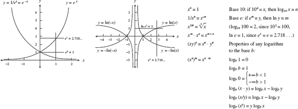
FIGURE C.3
C.6 Trigonometry
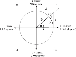
The angle θ subtended by an arc S of a circle of radius R is equal to the ratio θ = S/R, where θ is in radians. 1 radian = 180°/π = 57.296°, while 1° = π/180° = 0.17453 radians. If R is rotated counterclockwise from the positive x axis, θ is positive in sign. If R is rotated clockwise from the positive x axis, θ is negative in sign. The trigonometric functions of the angle θ are defined as specific ratios between the sides of the triangles shown in the figure and are expressed as
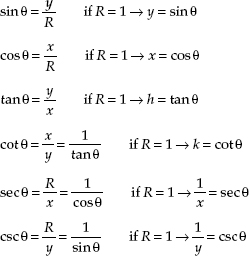
FIGURE C.4
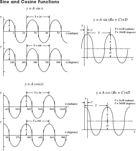
The graph of y = A sin θ is shown to the far left. To alter the vertical, horizontal, period, and phase of this function, alter the equation to the form y = A sin (Bx + C) + D. A is amplitude, 2π/B is the period (T), C is the phase shift, and D is the vertical shift. In electronics, a voltage can be expressed as
V0 is the peak voltage, Vdc is the dc offset, Φ is the phase shift, and ω is the angular frequency (rad/s), which is related to the conventional frequency (cycles/s) by
The graph of y = A cos x is shifted in phase by π/2 radians (or 90°) with respect to the graph y = A sin x. The following relations show how the sine and cosine functions are related:
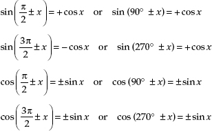
FIGURE C.5
C.7 Complex Numbers
Complex numbers are covered in detail in Chap. 2.
C.8 Differential Calculus
Say you have a function f(x). This function may represent a line, parabola, exponential curve, trigonometric curve, etc. Now pretend that you take a point and move it along the curve of f(x). At the same time, you envision a tangent line touching the curve at the point. As the point moves along the curve, the slope of the tangent line changes (“teeter-totters”)—provided the curve is not a line. Now, the slope of the tangent line has great significance in real-life situations. For example, if you graph a curve of the position of an object versus time, the slope at a particular time along the curve represents the instantaneous velocity of the object. Likewise, if you have an electrical charge versus time graph, the slope at time t represents the instantaneous current-flow. Now, the trick to finding the slope of a tangent line for any point along a curve involves using differential calculus. What differential calculus does is this: If you have a function, say, y = x2—through the tricks of differential calculus—you can find another function, which is called the derivative of y (usually expressed as y′ or dy/dx), that tells you the slope at every point along the curve of y. For y = x2, the derivative is dy/dx = 2x. If you are interested in the slope of y at x = 2, you plug 2 into dy/dx to give you a slope of 4. But how do you find the derivative of y = x2? Better yet, how do you find the derivative of any given function? The following provides the basic theory.
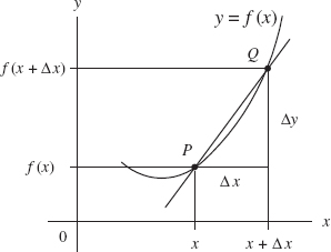
To find the derivative of a function y = f(x), you let P(x,y) be a point of the graph of y = f(x) and let Q(x + Δx, y + Δy) be another point of the graph. The slope of the line between P and Q is then simply
Now you substitute the function into the preceding equation. For example, if f(x) = x2, then f(x + Δx) = (x + Δx)2, and the whole expression equals [(x + Δx)2 – x2]/Δx. Next, you hold x fixed and let Δx approach zero. If the slope approaches a value that depends only on x, you call this the slope of the curve at point P. The slope of the curve at P is itself a function of x, defined at every value of x at which the limit exists. You denote the slope by f′(x) (“f prime”), or dy/dx (“dydx”), or df/dx (“dfdx”), and call any one of these terms (your choice) the derivative of f(x):
For the function f(x) = x2, after carrying out the limit, you would get f′(x) = dy/dx = 2x as the derivative.
FIGURE C.6
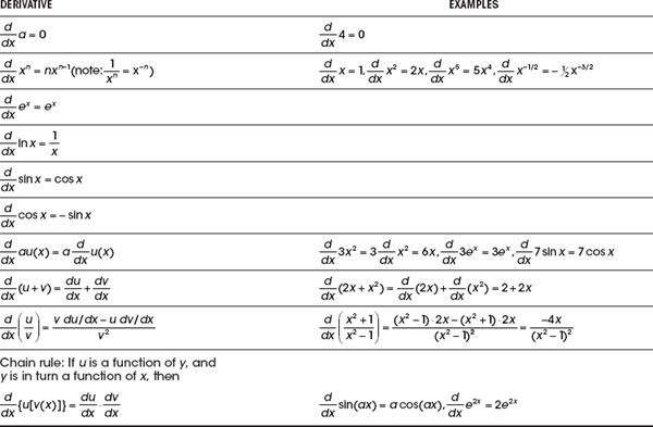
Now, in practice, if you need to find the derivative of a function, you do not bother using the preceding equation. To do so would be very time-consuming and might require a number of nasty mathematical tricks, especially if you are trying to find the derivative of a complex function such as 2ex sin (3x + 2). Instead, what you do is memorize a few simple rules and memorize a few simple derivatives. The table below shows some of the rules and simple derivatives that will come in handy for many applications. In the table, a and n are constants, while u and v are functions.
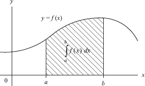
In differential calculus, our goal was to find the derivative of a function. In integral calculus, our goal is to find the functions of a derivative. In reality, calling one thing a derivative and another thing a function is somewhat confusing because a derivative is usually a function in itself. To avoid possible complications, we simply call anything that’s written as y = f(x) a function, call anything that’s written as dy/dx = df(x)/dx a derivative, and call anything that’s written as ∫ dy = ∫ f(x)dx an antiderivative or integral. In the last case, the “∫” is called the integral sign, the function f(x) is called the integrand, and dx is called the variable of integration. To integrate a function is to find all the functions that have it as a derivative—to find all of the given function’s antiderivatives. But, the term integration has a second, less technical meaning—to give the sum total of. In this meaning, integration represents a mathematical process that enables us to calculate the area of a region that has curved boundaries (see graph in Fig. C.7).
If we’re given an equation dy/dx = f(x) and wish to find y, we must integrate (antidifferentiate). In this case, we first rearrange the equation into the form dy = f(x)dx. Next, we integrate both sides:
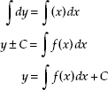
Again, ∫ is an integral sign, the function f(x) is the integrand, and C is the constant of integration. We guessed that ∫ dy = y ± C, since if we were to take the derivative of any function of the form y ± C (y + 2, y – 54, etc.) we’d get y as the answer—we worked backward. Since C could be positive or negative, it’s arbitrary to give it a sign. This way, we simply add C to the left. In this form, we call the integral an indefinite integral.
Example: Given dy/dx = 2, find y.
Example: Given dy/dx = 2, find y.

In real-life situations, it’s typically undesirable to have a constant in our answers, since we’re looking for a definite result. To get rid of the constant, we apply boundary conditions. For example, if we take our last example dy/dx = 2, we say we’re only interested in values of dy/dx from, say, 1 to 5—whatever range is appropriate for the situation. In that case, we take the definite integral
Without getting too technical, F represents the definite integral without the constant sign, while the (a) and (b) terms mean to place the boundaries points into the x term of F. If we consider our example dy/dx = 2 with boundary condition 1 to 5, we’d get:
We call this a definite integral. At this point, it’s worth introducing a graphical approach to visualizing integration. If we consider dy/dx = 2, and graph dy/dx versus x, we get a straight horizontal line at dy/dx = 2 for all values of x. By summing up the area under the curve, we get the integral. So incorporating the boundary conditions the area is (5 – 1) × 2 = 8.
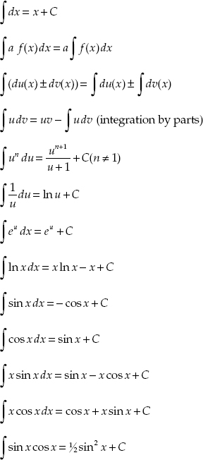
Now, if we attempt to integrate more complex functions, we’ll have a hard time guessing what the functions of the derivative are. Instead, we must apply some special tricks along the way. These tricks stem from a basic idea called the fundamental theorem of calculus, and they get fairly involved. Presenting the theory in such a short space isn’t going to do. However, in practice, you typically never use the fundamental theorem of calculus to find integrals of functions. Instead, you memorize a few fundamental integrals and learn a few tricks. The following list highlights some of the most common integrals and solutions. A mathematical handbook will provide a more extensive list. In the list, a u represents a function of x, while v represents another function of x.
FIGURE C.7
..................Content has been hidden....................
You can't read the all page of ebook, please click here login for view all page.