Chapter 6
Theory of the Wheel Shimmy Phenomenon
Chapter Outline
6.2. The Simple Trailing Wheel System with Yaw Degree of Freedom
6.1 Introduction
As an application of the theory developed in the previous chapter, we will study the self-excited oscillatory motion of a wheel about (an almost) vertical steering axis. This type of unstable motion is usually designated as the wheel shimmy oscillation. Shimmy is a violent and possibly dangerous vibration that may occur with front wheels of an automobile and with aircraft landing gears. Wobble of the front wheel of a motorcycle is an oscillatory unstable mode similar to shimmy. This steering vibration will be discussed in Chapter 11.
To investigate the shimmy phenomenon, the boundary of stability is established for system models of different degrees of complexity and we will examine the effect of employing different tire models. The linear stability analysis is extended to nonlinear systems which enables us to determine the limit of the shimmy amplitude (limit cycle) and the magnitude of initial disturbance or unbalance to initiate the self-excited oscillation. Much of the contents of the present chapter is based on the work of Von Schlippe and Dietrich (1941), Pacejka (1966,1981) and Besselink (2000).
Fromm, cf. Becker, Fromm and Maruhn (1931), is one of the first investigators who developed a theory for the shimmy motion of automobiles. Besides his advanced theoretical work, as a result of which the gyroscopic coupling between the angular motions about the longitudinal axis and about the steering axis was found to be the main factor causing shimmy, he has carried out and described, together with his co-workers Becker and Maruhn, some tests on a system with a rigid front axle. Also, Den Hartog (1940) and Rocard (1949) have treated this ‘gyroscopic’ shimmy for systems with live axles. The phenomenon was experimentally examined by Olley (1947).
Another kind of shimmy is closely related to tire and suspension lateral compliance and has been observed to occur with aircraft landing gears and automobiles equipped with independent front wheel suspensions. Many of the authors mentioned in connection with the development of non-steady-state out-of-plane tire models in Chapter 5 have used their model in connection with the analysis of the shimmy problem.
6.2 The Simple Trailing Wheel System with Yaw Degree of Freedom
First, the simplest system that can generate shimmy is discussed. Consider the trailing wheel system depicted in Figure 6.1. The vertical swivel axis moves along the ![]() axis with speed V. The motion variable is the yaw angle ψ of the wheel plane about the swivel axis. This axis intersects the road plane at a distance e (mechanical trail or caster length) in front of the contact center. The system is provided with a rotation damper with viscous damping coefficient k and possibly with a torsional spring with stiffness cψ. The moment of inertia about the swivel axis is denoted with I. This quantity varies with caster length e. However, we may consider a constant value of I if caster is accomplished by inclining the swivel axis about the wheel spin axis. If the caster angle remains relatively small, the camber angle that arises through steering may be neglected and the equations assuming a vertical axis will hold with good approximation.
axis with speed V. The motion variable is the yaw angle ψ of the wheel plane about the swivel axis. This axis intersects the road plane at a distance e (mechanical trail or caster length) in front of the contact center. The system is provided with a rotation damper with viscous damping coefficient k and possibly with a torsional spring with stiffness cψ. The moment of inertia about the swivel axis is denoted with I. This quantity varies with caster length e. However, we may consider a constant value of I if caster is accomplished by inclining the swivel axis about the wheel spin axis. If the caster angle remains relatively small, the camber angle that arises through steering may be neglected and the equations assuming a vertical axis will hold with good approximation.
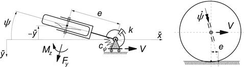
FIGURE 6.1 Simple trailing wheel system that is capable of showing shimmy. Two ways of realizing the mechanical caster length e of the contact center with respect to the steering axis (kingpin) have been indicated.
The tire will be considered massless and the contact line is approximated by a straight line tangent to the actual contact line at the leading edge (straight tangent approximation) for which the Eqns (5.125–5.127) hold or by a single point, Eqns (5.130–5.132), with and without the effect of tread width. The results will be compared with those obtained when using the almost exact Von Schlippe tire model. We have the equations:
![]() (6.1)
(6.1)
![]() (6.2)
(6.2)
![]() (6.3)
(6.3)
![]() (6.4)
(6.4)
![]() (6.5)
(6.5)
![]() (6.6)
(6.6)
![]() (6.7)
(6.7)
![]() (6.8)
(6.8)
![]() (6.9)
(6.9)
where a = 0 when the single contact point tire model is considered. To reduce the number of governing system parameters we will introduce the following nondimensional quantities (in bold letters) with the reference length ao representing the actual or the nominal half contact length:
 (6.10)
which includes the nondimensional pneumatic trail t = t/ao. After elimination of the time and all the variables except ψ and v1 in Eqns (6.1–6.9) and using the conversions (6.10) we obtain the nondimensional differential equations:
 (6.11)
The system is linear and of the third order. It is assumed that the tire deflection relaxation length σ = 3a or, with a = ao, nondimensionally: σ = 3. In the case of the single contact point tire model a must be taken equal to zero and σ must be given the value of σ + a = 4a. In the nondimensional notation σ takes the value of σ + a = σ + 1 = 4. For the pneumatic trail we assume t = 0.5a or t = 0.5.
The characteristic equation of system (6.11) becomes
![]() (6.12)
(6.12)
or
![]() (6.13)
(6.13)
In general, we may write
![]() (6.14)
(6.14)
According to the criterion of Hurwitz the conditions for stability of the motion of the third-order system read as follows:
• all coefficients ai of the characteristic equation must be positive:
![]() (6.15)
(6.15)
• the Hurwitz determinants Hn−1, Hn−3, etc. must be positive, which yields for the third order (n = 3) system:
![]() (6.16)
(6.16)
The first two coefficients of Eqn (6.13) are always positive. For the remaining coefficients, the conditions for stability become
![]() (6.17)
(6.17)
![]() (6.18)
(6.18)
while according to (6.16):
![]() (6.19)
(6.19)
It can be easily seen that, if the last two conditions are satisfied, the first one is satisfied automatically. If the condition an = a3 > 0 is the first to be violated then the motion turns into a monotonous unstable motion (divergent instability, that is, without oscillations). Consequently, if e < −(t + cψ) meaning that the steering axis lies a distance −e behind the contact center that is larger than t + cψ/CFα, the wheel swings around over 180 degrees to the new stable situation. If Hn−1 = H2 is the first to become negative, the motion becomes oscillatorily unstable. The boundaries of the two unstable areas are: a3 = 0 and H2 = 0.
In the case of vanishing damping (k = κ∗ = 0) condition (6.19) reduces to
![]() (6.20)
(6.20)
Apparently, in the (e, V) parameter plane the boundaries of (6.19) reduce to two parallel lines at e = σ + a and e = −t. When the caster lies in between these two values, the yaw angle performs an oscillation with exponentially increasing amplitude at any speed of travel. Apparently, when the damping is zero, the speed and the torsional stiffness do not influence the extent of the unstable area. They will, however, change the degree of instability and the natural frequency (eigenvalues).
If we have damping, the limit situation may be considered where the speed V tends to zero. The condition for stability then becomes
![]() (6.21)
(6.21)
which shows that the values for e become complex if σ cψ + κ∗ > ¼(t − a)2 + ta. This implies that in that case the unstable area becomes detached from the e axis.
In Figure 6.2 the unstable areas have been shown for different values of the viscous steer damping k and with steer stiffness cψ = 0. Damping reduces the size of the unstable area and pushes the extreme right-hand edge to lower values of speed. The curves resulting from the application of the straight tangent and the single contact point tire model approximations have been displayed together with the shaded curves representing the boundaries according to the almost exact Von Schlippe approximation. For a more detailed study of the situation at small values of V (< ca. 2), where at very low damping alternative stable and unstable ranges appear to arise when the exact theory is applied, we refer to Stepan (1997).
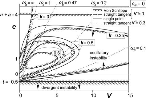
FIGURE 6.2 Areas of instability for the trailing wheel system of Figure 6.1 without steer stiffness at different levels of viscous steer damping. Consequences of using different tire models can be observed.
Appreciable deviations appear to occur at low values of speed V where the path frequency ωs is relatively high and thus the wavelength λ relatively short. This is in accordance with findings in Figure 5.23–5.27 where the frequency response functions according to various approximations have been compared. The straight tangent approximation shows a tendency to predict a shimmy instability that is somewhat too strong. On the other hand, the single point contact model turns out to be too stable: for k = 0.6 the unstable area vanishes all together. When employing the straight tangent approximation we at least appear to be on the safe side. For the case k = 0.5, a curve has been added in Figure 6.2 to show the effect of artificially introducing a proper value of κ∗ to improve the performance of the straight tangent model. The value κ∗ = CMφ = 0.6aCMα that corresponds to κ∗ = 0.3 indeed produces a better result. This is in accordance with the curve added in the Nyquist diagram of Figure 5.27 for CMφ = 0.6aCMα that shows an improved aligning torque frequency response.
The nondimensional path frequencies shown in the figure occur on the boundaries computed for the system with straight tangent approximation. Here the motion shows an undamped oscillation. Then, the solution of (6.13) contains a pair of purely imaginary roots. By replacing p by iωs in the characteristic equation and then separating the imaginary and the real terms we get two equations which can be reduced to one by eliminating the total damping coefficient kV + κ∗.
The resulting relationship between V and e has been shown for a number of values of ωs. At path frequency ωs = 1/√{σ(1 + t)} = 0.47 a special case arises where the frequency curve reduces to a straight line originating from (0,−t). By using one of the two equations, an expression for the nondimensional path frequency may be obtained:
![]() (6.22)
(6.22)
Figure 6.3 presents the diagram indicating the influence of damping due to tread width κ∗. This type of damping is especially effective at low speed. This is understandable because we have seen that the equivalent viscous damping coefficient decreases inversely proportionally with the forward velocity. The boundaries now have a chance to become closed at the left-hand side, cf. Eqn (6.21).
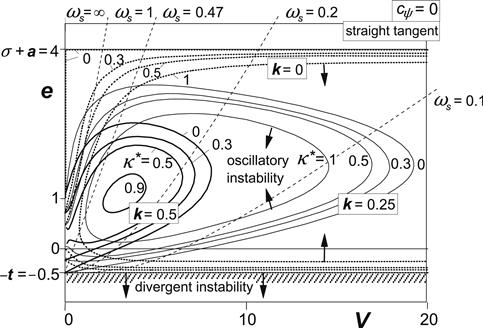
FIGURE 6.3 Areas of instability for the trailing wheel system of Figure 6.1 without steer stiffness. Influence of tread width damping at different levels of viscous steer damping.
As Figure 6.4 depicts, the steer torsional stiffness reduces the unstable shimmy area in size especially when sufficient damping is provided. At vanishing damping, the area of oscillatory instability appears to remain limited by the horizontal lines obtained from (6.20). The area of divergent instability is reduced through the restoring action of the torsional spring about the steering axis. Its upper boundary shifts downwards according to the negative trail −e = t + cψ.
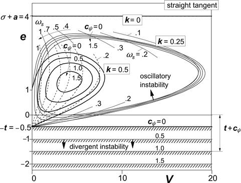
FIGURE 6.4 Influence of steer stiffness cψ on shimmy instability and on divergent instability at different levels of steer damping without tread width damping.
The influence of tire inertia has not been indicated in the diagrams. As may be expected from the diagram of Figure 5.38, which shows that the phase lag of the moment response is reduced through the action of the gyroscopic couple Mz,gyr especially at higher speeds, the area becomes limited at the right-hand side even in the absence of damping. Exercise 6.1 given below addresses this problem.
If the moment of inertia about the steering axis cannot be considered as a constant but rather as a function of the trail e, e.g., replace I by Iz + me2, then, considering the nondimensionalization defined by (6.10), the curves of the various diagrams must be reinterpreted: at a constant k the actual damping coefficient k is not a constant along the curve but increases with increasing e while at a given V the actual speed V diminishes at increasing e.
Example
Consider the system with parameters:
![]()
Speed of travel:
![]()
Shimmy wavelength:
![]()
so that at
![]()
and at
![]()
Shimmy frequency:
![]()
at V = 5.6 we have V = 33 m/s and according to the stability graph of Figure 6.3 (cψ = 0) we have at this speed and caster e = 0 a nondimensional path frequency ωs ≈ 0.12 so that ωs ≈ 0.85 rad/m, λ ≈ 7.3 m, ω ≈28 rad/s, and n ≈ 4.5 Hz. This would be the case at the boundary of stability where k ≈ 0.25 with κ∗ = 0.3. At about the same point in the diagram of Figure 6.4 we would have with a nondimensional steer stiffness cψ = 1 and damping coefficient k = 0.25 a nondimensional path frequency ωs ≈ 0.2 which yields ωs ≈ 1.4 rad/m, a wavelength λ ≈4.4 m and a frequency n ≈ 7.5 Hz.
Exercise 6.1. Influence of the Tire Inertia on the Stability Boundary
Consider the wheel system of Figure 6.1. Derive the stability conditions for this system with the inclusion of the effect of tire inertia approximated by the introduction of Mz,gyr (5.178). In nondimensional form, the gyroscopic couple becomes
![]() (6.23)
(6.23)
with
![]() (6.24)
(6.24)
cf. Eqns (5.59, 5.60) and (5.179).
Determine how the stability boundaries for the system without damping (κ∗ = k = cψ = 0) are changed due to the inclusion of the gyroscopic couple. Consider the following parameter values
![]()
Draw in the (e, V) diagram the boundaries for Cgyr = 0 and sketch the new stability boundary by calculating at least the boundary values for V at e = −t, e = 0 and e = 1 and, moreover, the boundary on the e-axis. Indicate where the system is stable.
6.3 Systems with Yaw and Lateral Degrees of Freedom
The additional degree of freedom that allows the kingpin to move sideways leads to a system which is of the fifth order. Figure 6.5 depicts the system with lateral compliance of the wheel suspension possibly associated with a torsional (camber) compliance with (virtual) axis of rotation assumed to be located at a height h above the ground (right-hand diagram). The inertia of the system (m, Iz) may be represented by two point masses mA and mB and a residual moment of inertia I∗ about the vertical axis. The two mass points are connected by a massless rod with length e, and are located on the wheel axis and the steer axis, respectively. Lateral damping will not be considered.
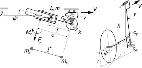
FIGURE 6.5 Lateral compliance introduced in the system.
The following set of equations hold for the dynamics of the system of Figure 6.5 assuming a vertical steering axis and adopting the straight tangent tire model, Eqns (5.125–5.127, 6.7):
![]() (6.25)
(6.25)
![]() (6.26)
(6.26)
![]() (6.2)
(6.2)
![]() (6.3)
(6.3)
![]() (6.4)
(6.4)
![]() (6.5)
(6.5)
![]() (6.6)
(6.6)
![]() (6.27)
(6.27)
![]() (6.8)
(6.8)
where the slip angle α is obtained from
![]() (6.28)
(6.28)
Before further studying the fifth-order system, let us try to reduce the system to a lower order while retaining the lateral compliance.
6.3.1 Yaw and Lateral Degrees of Freedom with Rigid Wheel/Tire (Third Order)
It can be shown that the lateral compliance of the wheel suspension has an effect that is similar to the effect of tire lateral compliance. The basic effect of lateral compliance of the suspension may be isolated by considering the wheel and tire as a rigid disk. As a result, slip angle α = 0 and a nonholonomic constraint equation arises that reduces the order of the system to three. Through this first-order differential equation, the condition that the wheel is unable to perform lateral slip is obeyed. We obtain the constraint equation from (6.28) with wheel slip angle α forced to be equal to zero:
![]() (6.29)
(6.29)
In addition, we assume that for the rigid disk the aligning torque and the contact length vanish:
![]() (6.30)
(6.30)
After elimination of Fy from the Eqns (6.25, 6.26) and expressing ![]() in terms of ψ and its derivative we find a third-order differential equation. Its characteristic equation with variable s reads as
in terms of ψ and its derivative we find a third-order differential equation. Its characteristic equation with variable s reads as
![]() (6.31)
(6.31)
The trivial condition against (divergent) instability that results from the last term of (6.31) which must remain positive becomes
![]() (6.32)
(6.32)
The condition for stability H2 > 0, cf. (6.16), reads as
![]() (6.33)
(6.33)
For the undamped case (k = 0) this reduces to the simple condition for stability, if e > 0:
![]() (6.34)
(6.34)
Apparently, a negative residual moment of inertia (I∗ < 0) will ensure stability. When f defines the location of the center of gravity behind the steer axis and i∗ denotes the radius of inertia of the combination (mA, mB, I∗), a negative residual moment of inertia would occur if i∗2 < f(e − f). For such a system, an increase of the lateral stiffness strengthens the stability.
If, on the other hand, I∗ > 0 a sufficiently large steer stiffness is needed to stabilize the system. It is surprising that a larger lateral stiffness may then cause the system to become unstable again.
The conclusion that the freely swiveling wheel system (that is, cψ = k = 0) is stable if the residual moment of inertia I∗ < 0 entails that when caster is realized by inclining the steering axis backwards (like in Figure 6.1 right-hand diagram) we have the situation that mA = 0 so that I∗ = I which is always positive. Consequently, for such a freely swiveling system equipped with a rigid thin tire the motion is always oscillatorily unstable.
6.3.2 The Fifth-Order System
The gyroscopic coupling terms that arise due to the angular camber velocity of the wheel system about the longitudinal axis located at a height h above the ground will be added to the Eqns (6.25, 6.26). For this, the coefficient βgyr is introduced:
![]() (6.35)
(6.35)
where Ip denotes the polar moment of inertia of the wheel. Furthermore, the ratio of distances with respect to the camber torsion center is introduced:
![]() (6.36)
(6.36)
Moreover, to fully account for the effects of the angular displacement about the longitudinal axis, which also arises when steering around an inclined kingpin (to provide caster), one may include the camber force in Eqn (6.2), and the small (negative) stiffness effects resulting from the lateral shift of the normal force Fz. Because of the fact that these effects are relatively small and appear to partly compensate each other, we will neglect the extra terms.
The differential equations that result when returning to the set Iz and m that replaces the equivalent set mA, mB, and I∗, and eliminating all variables except y, ψ and α′ read as
![]() (6.37)
(6.37)
![]() (6.38)
(6.38)
![]() (6.39)
(6.39)
In the equations, the lateral suspension damping, ky, has been included. In the further analysis, this quantity will be left out of consideration. To study the pure gyroscopic coupling effect, the ratio ζh will be taken equal to unity which would represent the case that the center of gravity and the lateral spring are located at ground level. For the special case that the center of gravity lies on the (inclined) steer axis, distance f = 0, the system description is considerably simplified. Our analysis will mainly be limited to this configuration. Besselink (2000) has carried out an elaborate study on the system of Figure 6.5 with the mass center located behind the (vertical) steering axis (f > 0), even behind the wheel center (f > e). For the complete results of this for aircraft shimmy important analysis we refer to the original publication. One typical result, however, where f = e will be discussed here.
The complete set of nondimensional quantities, extended and slightly changed with respect to the set defined by Eqn (6.10), reads as
 (6.40)
Here, s denotes the nondimensional Laplace variable. The nondimensional differential equations follow easily from the original Eqns (6.37–6.39). For the stability analysis, we need the characteristic equation which reads in nondimensional form:
![]() (6.41)
(6.41)
The coefficients of (6.41) with f = ky = 0 are
![]()
![]()
![]()
![]()
![]()
![]() (6.42)
(6.42)
The influence of a number of nondimensional parameters will be investigated by changing their values. The other parameters will be kept fixed. The values of the fixed set of parameters are
![]() (6.43)
(6.43)
For the fifth-order system the Hurwitz conditions for stability read as:
• all coefficients ai of the characteristic equation must be positive:
![]() (6.44)
(6.44)
• the Hurwitz determinants Hn−3 and Hn−1 must be positive, which yields:
 (6.45)
It turns out that for the case without damping and gyroscopic coupling terms (k = κ∗ = βgyr = 0), a relatively simple set of analytical expressions can be derived for the conditions of stability. It can be proven that when a5 > 0, H2 > 0, H4 > 0 the other conditions are satisfied as well. Consequently, the governing conditions for stability of the system without damping and gyroscopic coupling read as:
![]() (6.46)
(6.46)
![]() (6.47)
(6.47)
![]() (6.48)
(6.48)
We may ascertain that for the special case of a rigid wheel where CFα →∞ and a, σ, t → 0 the condition (6.46) corresponds with (6.32) and the condition
![]() (6.49)
(6.49)
that results from (6.48) corresponds with condition (6.34) if we realize that in the configuration studied here we have: mA = 0 and I∗ = Iz.
For the case with an elastic tire with stability conditions (6.46–6.48) we will present stability diagrams and show the effects of changing the stiffnesses. In addition, but then necessarily starting out from Eqns (6.42, 6.44, 6.45), the influence of the steer and tread damping and that of the gyroscopic coupling terms will be assessed.
First, let us consider the system with lateral suspension compliance but without steer torsional stiffness, cψ = 0, that is, a freely swiveling wheel possibly damped (governed by the combined coefficient k + κ∗/V) and subjected to the action of the gyroscopic couple (that arises when the lateral deflection is connected with camber distortion as governed by a nonzero coefficient βgyr). From the above conditions it can be shown that for the simple system without damping and camber compliance stability may be achieved only at the academic case of large caster e > a + σ when the lateral stiffness of the wheel suspension is sufficiently large:
![]() (6.50)
(6.50)
The minimum stiffness where stability may occur is
![]() (6.51)
(6.51)
with iz representing the radius of inertia:
![]() (6.52)
(6.52)
The value of the caster length ec where stability commences (at cy,crit) is
![]() (6.53)
(6.53)
Consequently, it may be concluded that with respect to the third-order system of Figure 6.2 the introduction of lateral suspension compliance shifts the upper boundary of the area of instability to values of caster length e larger than a + σ. At the same time, a new area of instability emerges from above. When the lateral stiffness becomes lower than the critical value (6.51) the stable area vanishes altogether at e = ec.
The case with steer and tread damping shows ranges of stability that vary with speed of travel V. In Figure 6.6 areas of instability have been depicted for different values of the lateral stiffness. The upper left inset illustrates the case without damping. At vanishing lateral stiffness a narrow range of stability appears to remain in the negative trail range with a magnitude smaller than the pneumatic trail t.
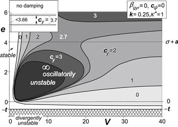
FIGURE 6.6 Influence of lateral suspension compliance with nondimensional stiffness cy on stability. Gyroscopic couple and steer stiffness not regarded. No-dimensional parameters: f = 0, m = 0.5, t = 0.5, σ = 3.
When a finite height h of the longitudinal torsion axis is considered, parameter βgyr defined by (6.35) obtains a value larger than zero. For βgyr = 0.2 the diagram of Figure 6.7 arises. An important phenomenon appears to occur that is essential for this two degree of freedom system (not counting the ‘half’ degree of freedom stemming from the flexible tire). A new area of instability appears to show up at higher values of speed. The area increases in size when the lateral (camber) stiffness decreases. At the same time, the original area of oscillatory instability shrinks and ultimately vanishes. Around zero caster stable motions appear to become possible for all values of speed when a (near) optimum lateral stiffness is chosen. The high-speed shimmy mode exhibits a considerably higher frequency than the one occurring in the lower speed range of instability. This is illustrated by the nondimensional frequencies indicated for the case cy = 2 at e = 0.5. The corresponding nondimensional wavelength λ = λ/a is obtained by using the formula: λ = 2π V/ω. In Table 6.1 the nondimensional frequencies ω, wavelengths λ, and path frequencies 1/λ = a/λ have been presented as computed for the four different values of nondimensional velocities where the transition from stable to unstable or vice versa occurs. Also, the mode of vibration is quite different for this ‘gyroscopic’ shimmy exhibiting a considerably larger lateral motion amplitude of the wheel contact center with respect to the yaw angle amplitude than in the original ‘lateral (tire) compliance’ shimmy mode. To illustrate this, the table shows the ratio of amplitudes of the lateral displacement of the contact center (cf. Figure 6.5) and the yaw angle multiplied with half the contact length: aψ. For the two lower values of speed, the lateral displacement appears to lag behind the yaw angle with about 135° while for the two higher speeds the phase lag amounts to about 90°.
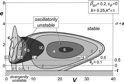
FIGURE 6.7 Influence of lateral (camber) suspension compliance with gyroscopic coupling. Steer stiffness is equal to zero. At increasing compliance 1/cy, a new area of oscillatory instability shows up while the original area shrinks. Frequencies have been indicated for the case cy = 2 at e = 0.5.
TABLE 6.1 Nondimensional Frequencies, Wavelengths and Ratio of Amplitudes of Lateral Displacement at Contact Center and Yaw Angle ψ Times Half-Contact Length a for Speeds at Stability Boundaries as Indicated in Figure 6.7 at Trail e = 0.5
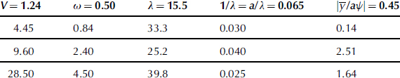
Figure 6.8 depicts the special case of vanishing damping for a number of values of the lateral stiffness. At caster near or equal to zero limited ranges of speed with stable motions appear to occur. These speed ranges correspond with the stable ranges in between the unstable areas of Figure 6.7 (if applicable). For the indicated points A and B and for a number of neighboring points the eigenvalues and eigen-vectors have been assessed and shown in Figures 6.22, 6.23 in Section 6.4.1 where the energy flow is studied.
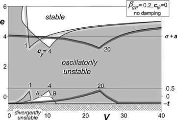
FIGURE 6.8 Influence of lateral (camber) suspension compliance with gyroscopic coupling. Steer stiffness is equal to zero. Steer and tread damping equal to zero. Eigenvalues and eigen-vectors of points A and B are analyzed in Figures 6.22, 6.23.
The system will now be provided with torsional steer stiffness cψ. For the undamped case, the conditions (6.46–6.48) hold to ensure stability. It can be observed that except for the condition (6.46) cψ appears in combination with cy in the factor cψ − cy/m. We may introduce an effective yaw stiffness and an effective lateral stiffness:
![]() (6.54)
(6.54)
and establish a single diagram for the ranges of stability for the two effective stiffnesses as presented in Figure 6.10. The way in which the boundaries are formed may be clarified by the diagram of Figure 6.9. The parabola represents the variation of the second Hurwitz determinant H2 divided by m2 V, cf. Eqn (6.47), as a function of the caster length e. This same term also appears in the expression for the fourth Hurwitz determinant H4 according to (6.48). For both cases ![]() and
and ![]() the straight line originating from the point (σ + a, 0) at a slope
the straight line originating from the point (σ + a, 0) at a slope ![]() and
and ![]() , respectively, have been depicted. The points of intersection with the parabola correspond to values of e where H4 = 0. Depending on the signs of factor e + t and of H2 and a5 the ranges of stability can be found. Five typical cases A–E have been indicated. They correspond to similar cases indicated in Figure 6.10. Case D at small negative e lies inside the small stable triangle of Figure 6.10. Here
, respectively, have been depicted. The points of intersection with the parabola correspond to values of e where H4 = 0. Depending on the signs of factor e + t and of H2 and a5 the ranges of stability can be found. Five typical cases A–E have been indicated. They correspond to similar cases indicated in Figure 6.10. Case D at small negative e lies inside the small stable triangle of Figure 6.10. Here ![]() > 0, e + t > 0 and H2/m2 V >
> 0, e + t > 0 and H2/m2 V > ![]() (σ + a − e). Case C shows a range of e where H4 > 0 but at the same time H2 < 0 so that instability prevails. For larger negative values of the caster stability arises because e + t changes sign while a5 remains positive. Also for larger values of
(σ + a − e). Case C shows a range of e where H4 > 0 but at the same time H2 < 0 so that instability prevails. For larger negative values of the caster stability arises because e + t changes sign while a5 remains positive. Also for larger values of ![]() a stable area appears to show up for e < −t. For cases like D and E, stability occurs for large values of the mechanical trail e (not very realistic for our present assumption that f = 0 which means: c.g. on (inclined) steering axis). In a similar large range of e stability occurs for large effective lateral stiffness, e.g., case A. This case has already been referred to previously when discussing the situation without steer stiffness, cf. Figure 6.6 upper left inset, Eqn (6.50). Case B shows instability for all values of e. As has been indicated in Figure 6.10, we can establish the abscissa cψ by shifting the vertical axis to the left over a distance cy/m. At the left of the shifted axis the steer stiffness must be considered equal to zero so that
a stable area appears to show up for e < −t. For cases like D and E, stability occurs for large values of the mechanical trail e (not very realistic for our present assumption that f = 0 which means: c.g. on (inclined) steering axis). In a similar large range of e stability occurs for large effective lateral stiffness, e.g., case A. This case has already been referred to previously when discussing the situation without steer stiffness, cf. Figure 6.6 upper left inset, Eqn (6.50). Case B shows instability for all values of e. As has been indicated in Figure 6.10, we can establish the abscissa cψ by shifting the vertical axis to the left over a distance cy/m. At the left of the shifted axis the steer stiffness must be considered equal to zero so that ![]() . The stability boundary a5 = 0 shifts to the left together with the cψ = 0 axis.
. The stability boundary a5 = 0 shifts to the left together with the cψ = 0 axis.
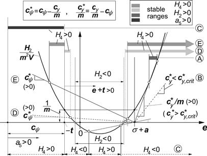
FIGURE 6.9 Establishing the ranges of stability using the conditions (6.46–6.48) which hold for the fifth-order system without damping and gyroscopic coupling. The cases A–E correspond to those indicated in the stability diagram of Figure 6.10.
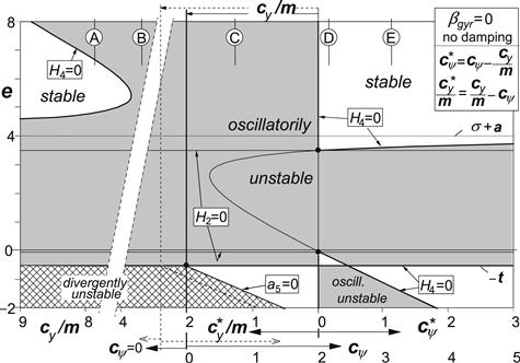
FIGURE 6.10 Basic stability diagram according to conditions (6.46–6.48) for the fifth-order system without damping and gyroscopic coupling. The cases A–E correspond to those indicated in the stability diagram of Figure 6.9. The diagram holds in general, the case with cy/m = 2 is an example, note: m = 0.5.
In Figure 6.11 the diagram of Figure 6.10 is repeated but only for the version with cψ as abscissa and for one fixed value of cy. Figures 6.12 and 6.13 clearly show the influence of damping. The stable areas increase in size, while the unstable area tends to split itself into two parts, the higher stiffness part of which (cψ > ∼cy/m) appears to vanish at sufficient damping. Also in the low yaw stiffness range the instability is suppressed especially in the lower range of speed. For a caster length close to zero it appears possible to achieve stability through adapting the steer stiffness (making it a bit larger than cy/m, cf. Case D of Figure 6.10) and/or by supplying sufficient damping.
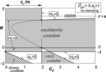
FIGURE 6.11 Stability diagram according to Figure 6.10 with steer stiffness along abscissa, at a fixed value of the lateral stiffness, without damping or gyroscopic coupling.
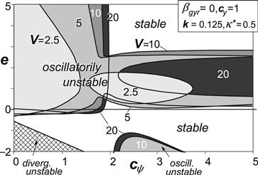
FIGURE 6.12 Same as Figure 6.11 but with some damping. Areas of instability at different levels of speed.
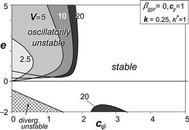
FIGURE 6.13 Same as Figure 6.12 but with more damping.
The more complex situation where gyroscopic coupling is included has been considered in Figures 6.14–6.16. For vanishing steer stiffness, cψ → 0, the situation of Figures 6.8, 6.7 is reached again. In Figure 6.14 where the damping is zero, the curve at low speed resembles the graph of Figure 6.11. As was observed to occur in the zero yaw stiffness case, we see that in the lower yaw stiffness range (cψ < ∼cy/m) an optimum value of the speed appears to exist where the unstable e range becomes smallest or vanishes altogether (at sufficient damping). In the higher stiffness range, increasing the speed promotes shimmy except in the negative e range where the opposite may occur. In this same range of yaw stiffness an increase of the stiffness appears to lower the tendency to shimmy.
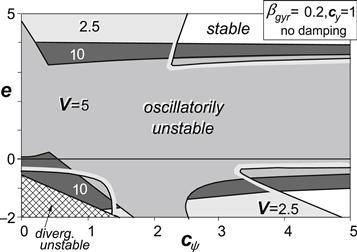
FIGURE 6.14 Diagram for the case of Figure 6.11 but with gyroscopic coupling. Areas of instability at different levels of speed.
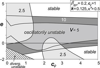
FIGURE 6.15 Same as Figure 6.14 but with some damping.
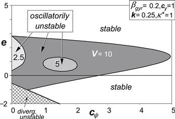
FIGURE 6.16 Same as Figure 6.15 but with more damping.
Besselink (2000) has analyzed the more general and for aircraft landing gears more realistic configuration where the center of gravity of the swiveling part is located behind the steering axis. Notably, the case where f = e and the peculiar case with f > e which may be beneficial to suppress shimmy. For the configuration that f = e and damping and gyroscopic coupling are disregarded, the following conditions for stability hold:
![]() (6.55)
(6.55)
![]() (6.56)
(6.56)
![]() 6.57)
6.57)
with the two parabolic functions of e:
![]() (6.58)
(6.58)
![]() (6.59)
(6.59)
Figure 6.17 depicts the boundaries of stability according to the above functions. The ordinates of two characteristic points have already been given in the figure. For the three other points, we have the e values:
![]() (6.60)
(6.60)
![]() (6.61)
(6.61)
![]() (6.62)
(6.62)
The appearance of the stability diagram is quite different with respect to that of Figure 6.11 where f = 0. Still, an area of instability exists in between the levels of the trail: −t < e < σ + a. Like in the f = 0 case (clearly visible in Figure 6.12), we have two different ranges of instability: area 1 and area 2 where different modes of unstable oscillations occur. In the range of the caster length −t < e < σ + a these areas correspond to the lower and the higher yaw stiffness regions.
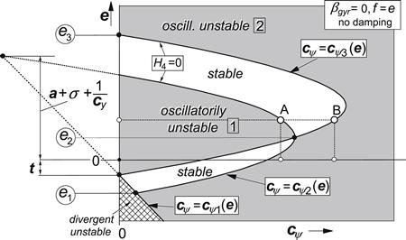
FIGURE 6.17 Basic stability diagram for the case f = e (c.g. distance e behind steer axis). Steer and tread damping are equal to zero. Gyroscopic coupling is disregarded. The functions cψi(e) are defined by Eqns (6.55, 6.58, 6.59). Eigenvalues and eigen-vectors of points A and B are analyzed in Figures 6.18, 6.19. (From: Besselink 2000).
For the points A and B which lie on the boundaries of the lower and the higher stiffness instability areas, respectively, the modes of vibration have been analyzed. The conditions for stability (6.55–6.57) of the undamped system without gyros are independent of the speed. When changing the speed of travel the damping of the mode that is just on a boundary of instability remains equal to zero. The other mode shows a positive damping which changes with speed as does the frequency of this stable mode. In Figures 6.18 and 6.19 (from Besselink 2000), the damping, frequency, amplitude ratio, and phase lead of the lateral displacement of the contact center ![]() with respect to the yaw angle ψ have been presented for the two modes of vibration – in Figure 6.18 for case A and in Figure 6.19 for case B of Figure 6.17. Using a reference tire radius rref the quantities
with respect to the yaw angle ψ have been presented for the two modes of vibration – in Figure 6.18 for case A and in Figure 6.19 for case B of Figure 6.17. Using a reference tire radius rref the quantities ![]() and
and ![]() have been defined as follows:
have been defined as follows: ![]() = y/rref [−],
= y/rref [−], ![]() = V/rref [1/sec]. From the graphs can be observed that the lower yaw stiffness case A shows a mode on the verge of instability (mode 1) that has a lower frequency and a larger amplitude ratio |
= V/rref [1/sec]. From the graphs can be observed that the lower yaw stiffness case A shows a mode on the verge of instability (mode 1) that has a lower frequency and a larger amplitude ratio |![]() /ψ| than mode 2 in case B. Evidently, case B exhibits a more pronounced yaw oscillation, whereas the motion performed by mode 1 of case A comes closer to a lateral translational oscillation. The next section discusses the mode shapes of these periodic motions in relation with the energy flow into the unstable system.
/ψ| than mode 2 in case B. Evidently, case B exhibits a more pronounced yaw oscillation, whereas the motion performed by mode 1 of case A comes closer to a lateral translational oscillation. The next section discusses the mode shapes of these periodic motions in relation with the energy flow into the unstable system.
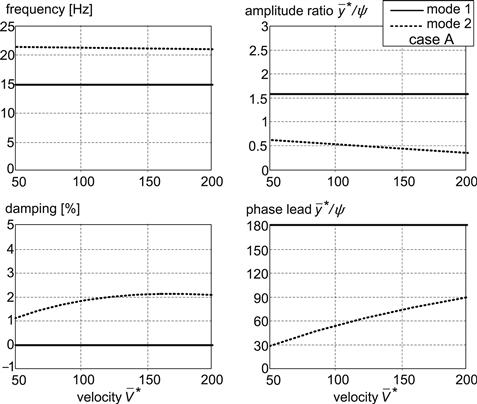
FIGURE 6.18 Natural frequencies, damping and mode shapes for case A of Figure 6.17.
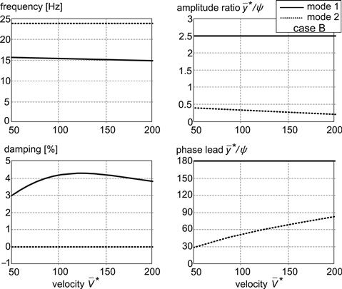
FIGURE 6.19 Natural frequencies, damping and mode shapes for case B of Figure 6.17.
Besselink has analyzed the effects of changing a number of parameters of a realistic two-wheel, single axle main landing gear model configuration (of civil aircraft, also see Van der Valk 1993). Degrees of freedom represent axle yaw angle, strut lateral deflection, axle roll angle, and tire lateral deflection (straight tangent). This makes the total order of the system equal to seven. Important conclusions regarding the improvement of an existing system aiming at avoidance of shimmy have been drawn. Two mutually different configurations have been suggested as possible solutions to the problem, with the c.g. position f assumed to remain equal to the trail e.
• large positive trail (e > 0):
‘An increase of the mechanical trail and a reduction of the lateral stiffness are required to improve stability at high forward velocity. Increasing the yaw stiffness will generally improve the shimmy stability of a gear with a positive mechanical trail provided that some structural damping is present. A limited reduction of the roll stiffness improves the stability at high forward velocities. The yaw moment of inertia should be kept as small as possible in case of a large positive mechanical trail’.
• small negative trail (e < 0):
‘For a landing gear with a negative trail an upper boundary exists for the yaw stiffness. The actual value of this stiffness may be quite low: for the baseline configuration, the yaw stiffness would have to be reduced almost by a factor 3 to obtain a stable configuration with a negative trail. A relatively small increase in track width relaxes this requirement considerably. If the absolute value of the negative trail equals the pneumatic trail, there exists no lower limit for the yaw stiffness to maintain stability. The effect of increasing the lateral stiffness is quite similar to increasing the track width and improves the shimmy stability in case of negative trail’.
In comparison with the baseline configuration, the proposed modifications result in a major gain in stability. This illustrates that it may be possible to design a stable conventional landing gear, provided that the combination of parameter values is selected correctly.
For detailed information also on the results of simulations with a multi-body complex model in comparison with full-scale experiments on a landing aircraft exhibiting shimmy we refer to the original work of Besselink (2000).
6.4 Shimmy and Energy Flow
To sustain the unstable shimmy oscillation, energy must be transmitted ‘from the road to the wheel’. We realize that, ultimately, the power can only originate from the vehicle's propulsion system. The relation between unstable modes and the self-excitation energy generated through the road to tire side force and aligning moment is discussed in detail in Subsection 6.4.1. The transition of driving energy (or the vehicle forward motion kinetic energy) to self-excitation energy is analyzed in Subsection 6.4.2. Obviously, besides, for the supply of self-excitation energy, the driving energy is needed to compensate for the energy that is dissipated through partial sliding in the contact patch.
6.4.1 Unstable Modes and the Energy Circle
To start out with the problem matter let us consider the simple trailing wheel system of Figure 6.1 with the yaw angle ψ representing the only degree of freedom of the wheel plane. If the mechanical trail is equal to zero it is only the aligning torque that exerts work when the wheel plane is rotated about the steering axis. If the yaw angle varies harmonically
![]() (6.63)
(6.63)
The moment response becomes for small path frequency ωs approximately:
![]() (6.64)
(6.64)
where the phase angle follows, for instance, from transfer functions (5.110) or (5.113) or Table 5.1 (below Figure 5.27):
![]() (6.65)
(6.65)
The negative value of which corresponds to the fact that the moment lags behind the yaw angle. The energy transmitted during one cycle can be found as follows (θ = ωss):
![]() (6.66)
(6.66)
Apparently, because of the negative phase angle the work done by the aligning torque is positive which means that energy is fed into the system. As a result, the undamped wheel system will show unstable oscillations which is in agreement with our earlier findings. It is of interest to note that in contrast to the above result that holds for a tire, a rotary viscous damper (with a positive phase angle of 90°) shows a negative energy flow which means that energy is being dissipated.
If we would consider a finite caster length e, more self-excitation will arise due to the contribution of the side force that also responds to the yaw angle with phase lag. At the same time, however, a part of Fy will now respond to the slip angle and, consequently, damps the oscillation. The slip angle arises as a result of the lateral slip speed which is equal to the yaw rate times the caster length. Finally, at e = σ + a, the moment and the side force are exactly in phase with the yaw angle (cf. situation depicted in Figure 5.6) and the stability boundary is reached. At e = −t the moment about the steer axis vanishes if the simplified straight tangent or single contact point model is used. This also implies that the boundary of oscillatory instability is attained.
We will now turn to the much more complicated system with lateral compliance of the suspension included. The two components of the periodic oscillatory motion of the wheel that occurs on the boundary of (oscillatory) instability may be described as follows:
![]() (6.67)
(6.67)
![]() (6.68)
(6.68)
The quantity η represents the amplitude ratio, ξ; indicates the phase lead of the lateral motion with respect to the yaw motion and θ equals ωt or ωss. The energy W that flows from the road to the wheel during one cycle is equal to the work executed by the side force and the aligning torque that act on the moving wheel plane. Hence, we have
![]() (6.69)
(6.69)
when W > 0 energy flows into the system and if the system is considered to be undamped (k = κ∗ = 0) the conclusion must be that the motion is unstable. Ultimately, the energy must originate from the power delivered by the vehicle propulsion system. How this transfer of energy is realized will be treated in the next section.
To calculate the work done, the force and moment are to be expressed in terms of the wheel motion variables (6.67, 6.68). For this, a tire model is needed and we will follow the theory developed by Besselink (2000) and take the straight tangent approximation of the stretched string model, which is governed by the Eqns (6.2, 6.4, 6.6, 6.7). For the periodic response of the transient slip angle α′ to the input motion (6.67, 6.68) the following expression is obtained:
![]() (6.70)
(6.70)
with the expressions (6.2, 6.4) for the force and the moment the integral (6.69) becomes
![]() (6.71)
(6.71)
On the boundary of stability W = 0 and for a given path frequency ωs or wavelength λ = 2π/ωs a relationship between η and ξ; results from (6.71). To establish the functional relationship it is helpful to switch to Cartesian coordinates:
![]() (6.72)
(6.72)
The expression for the energy now reads as
![]() (6.73)
(6.73)
Apparently, for a given value of W this represents the description of a circle. For W = 0 and after the introduction of the wavelength λ as parameter the function takes the form
![]() (6.74)
(6.74)
When the mode shape of the motion of the wheel plane defined by η and ξ; or by xp and yp is such that (6.74) is satisfied, the motion finds itself on the boundary of stability. The center of Besselink's energy circle is located at
![]() (6.75)
(6.75)
From (6.74) it can be ascertained that independent of λ the circles will always pass through the two points on the xp axis: xp = −(σ + a) and xp = t. We have now sufficient information to construct the circles with λ as parameter. In Figure 6.20, these circles have been depicted together with circles that arise when different tire models are used. As expected, the circles for the more exact tire models deviate more from those resulting from the straight tangent tire model when the wavelength becomes smaller. These circles that arise also for other massless models of the tire can be easily proven when considering the fact that at a given wavelength we have a certain amplitude and phase relationship of the force Fy and the moment ![]() with respect to the two input motion variables
with respect to the two input motion variables ![]() and ψ. That the circles pass through the point (−σ −a, 0) follows from the earlier finding that the response of all ‘thin’ tire models when the wheel is swiveled around a vertical axis that is positioned a distance σ + a in front of the wheel axle (cf. Figure 5.6) are equal and correspond to the steady-state response.
and ψ. That the circles pass through the point (−σ −a, 0) follows from the earlier finding that the response of all ‘thin’ tire models when the wheel is swiveled around a vertical axis that is positioned a distance σ + a in front of the wheel axle (cf. Figure 5.6) are equal and correspond to the steady-state response.
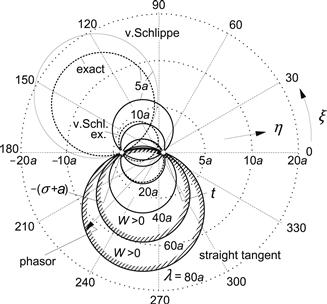
FIGURE 6.20 Mode shape plot (amplitude ratio η, phase ξ;) with Besselink's zero energy circles for different wavelengths and tire model approximations, indicating mode shapes for which shimmy begins to show up (instability occurs if at a particular value of the motion wavelength λ the phasor end point gets inside the corresponding circle). At smaller wavelengths the circle belonging to the straight tangent approximation begins to appreciably deviate from the exact or Von Schlippe representation.
When parameters of the system are changed and the mode shape is changed so that the end point of the phasor with length η and phase angle ξ; moves from outside the circle to the inside, the system becomes oscillatory unstable. It becomes clear that depending on the wavelength a whole range of possible mode shapes of the wheel plane motion is susceptible to forming unstable shimmy oscillations.
As an example, the situation that arises with the cases A and B of Figures 6.17–6.19 has been depicted in Figure 6.21. In case A mode 1 is on the verge of becoming unstable. The mode shape corresponds to the motion indicated in Figure 5.6 and remains unchanged when the speed is varied. The circles, however, change in size and position when the speed is changed which correspond to a change in wavelength. Mode 2 appears to remain outside the circles indicating that this particular mode is stable. In case B mode 1 is stable and mode 2 sits on the boundary of stability. This is demonstrated in the right-hand diagram where the end point of the phasor of mode 2 remains located on the (changing) circles when the speed is changed.
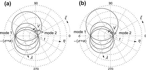
FIGURE 6.21 Zero energy circles for the cases A and B of Figure 6.17, indicating the mode shape of mode 1 at the boundary of stability in case A and the same for mode 2 in case B.
As a second example we apply this theory to the configuration with f = 0 with the gyroscopic coupling included. In Figure 6.8 the cases A and B have been indicated at a trail e = 0. Because of the gyroscopic action the condition for stability is speed dependent, although damping is assumed equal to zero. This makes it possible to actually see that the zero energy circle is penetrated or exited when the speed is increased.
In Figures 6.22 and 6.23 the phasors (here considered as complex quantities) have been indicated for a number of values of the nondimensional speed V. The nondimensional wavelength and eigenvalue of the mode considered change with speed as have been indicated in the respective diagrams. Cases A and B (with respectively mode 1 and 2 on the boundary of stability) have been marked. When the speed is increased from 6 to 14, two boundaries of stability (A and B) are passed in between which according to Figure 6.8 a stable range of speed exists. In Figure 6.22 we see that in accordance with this the phasor of mode 1 first lies inside the circle (belonging to V = 6 with frequency ω = 0.66 and corresponding wavelength λ = 57a) then crosses the circle at V = 9.05 (A) and finally ends up at a speed V = 14 outside the circle meaning that this mode is now stable. At the same time, following mode 2 in Figure 6.23, we observe that first the mode point lies outside the circle at V = 6 (now for the different frequency ω = 2.99 and wavelength λ = 12.6a), crosses the circle at V = 11.2 (B) and moves to the inside of the circle into the unstable domain. From the eigenvalues s the change in damping and frequency can be observed. The mode shapes are quite different for the two modes. Mode 1 shows a relatively small lateral displacement ![]() with respect to the yaw angle multiplied with half the contact length aψ. At first
with respect to the yaw angle multiplied with half the contact length aψ. At first ![]() slightly lags behind ψ which turns into a lead at higher speeds. Mode 2 shows a higher frequency and smaller wavelength while
slightly lags behind ψ which turns into a lead at higher speeds. Mode 2 shows a higher frequency and smaller wavelength while ![]() is relatively large and lags behind ψ.
is relatively large and lags behind ψ.
Exercise 6.2. Zero Energy Circle Applied to the Simple Trailing Wheel System
Consider the third-order system of Figure 6.1 described by the Eqns (6.1–6.9) but without damping: k = κ∗ = 0. Establish the reduced expression for the work W from the general formula (6.69). Show that the stability condition H2 > 0 corresponds to W < 0 which means that the mode shape point lies outside the zero energy circle.
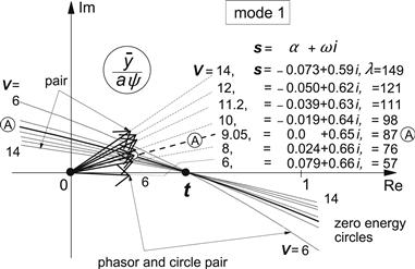
FIGURE 6.22 System of Figure 6.8 with gyroscopic coupling making stability speed dependent. Circle segments and phasors of mode shapes of mode 1 for a series of speed values covering the range in which points A and B of Figure 6.8 are located. At increasing speed the phasor crosses the circle at V = 9.05 into the stable domain.
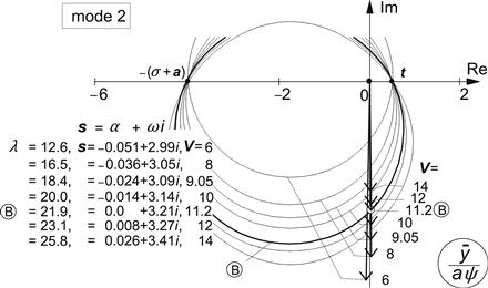
FIGURE 6.23 Circles and phasors of mode shapes of mode 2 for same series of speed values as in Figure 6.22. At increasing speed, the phasor crosses the circle at V = 11.2 toward its inside which means: entering the unstable domain.
6.4.2 Transformation of Forward Motion Energy into Shimmy Energy
The only source that is available to sustain the self-excited shimmy oscillations is the vehicle propulsion unit. The tire side force has a longitudinal component that when integrated over one shimmy cycle must be responsible for an average drag force that is balanced by (a part of) the vehicle driving force.
In the previous section, we have seen that the work done by the side force and the aligning torque is fed into the system to generate the shimmy oscillation. The link that apparently exists between self-excitation energy and driving energy will be examined in the present section. For this analysis, dynamic effects may be left out of consideration. The wheel is considered to roll freely (without braking or driving torques).
During a short span of traveled distance ds of the wheel center, the wheel plane moves sideways over a distance d![]() and rotates about the vertical axis over the increment of the yaw angle dψ. At the same time, the tire lateral deflection is changed and, when sliding in the contact patch is considered, some elements will slide over the ground. Consequently, we expect that the supplied driving energy dE is equal to the sum of the changes of (self-)excitation energy dW, tire potential energy dU and tire dissipation energy dD.
and rotates about the vertical axis over the increment of the yaw angle dψ. At the same time, the tire lateral deflection is changed and, when sliding in the contact patch is considered, some elements will slide over the ground. Consequently, we expect that the supplied driving energy dE is equal to the sum of the changes of (self-)excitation energy dW, tire potential energy dU and tire dissipation energy dD.
In Figure 6.24 the tire is shown in a deflected situation. We have the pulling force Fd acting in forward ![]() direction from vehicle to the wheel axle and furthermore the lateral force Fe and yaw moment Me from rim to tire. These forces and moment are in equilibrium with the side force Fy and aligning torque Mz which act from road to tire. A linear situation is considered with small angles and a vanishing length of the sliding zone. For the sake of simplicity, we consider an approximation of the contact line according to the straight tangent concept.
direction from vehicle to the wheel axle and furthermore the lateral force Fe and yaw moment Me from rim to tire. These forces and moment are in equilibrium with the side force Fy and aligning torque Mz which act from road to tire. A linear situation is considered with small angles and a vanishing length of the sliding zone. For the sake of simplicity, we consider an approximation of the contact line according to the straight tangent concept.
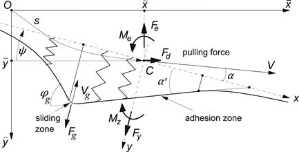
FIGURE 6.24 On the balance of driving, self-excitation, and dissipation energy.
Energy is lost due to dissipation in the sliding zone at the trailing edge of the contact zone. To calculate the dissipated energy, we need to know the frictional force and the sliding velocity distance. For the bare string model, we have the concentrated force Fg that acts at the rear edge and that is needed to maintain the kink in the deformation of the string. This force is equal to the difference of the slopes of the string deflection just behind and in front of the rear edge times the string tension force S = ccσ2. For the straight tangent string deformation with transient slip angle or deformation gradient ![]() the slope difference is equal to φg = 2(σ + a) α′/s. The force becomes: Fg = 2ccσ(σ + a) α′. The average sliding speed Vg over the vanishing sliding range is equal to half the difference in slope of the string in front and just passed the kink times the forward speed V. This multiplied with the time needed to travel the distance ds gives the sliding distance sg. We find for the associated dissipation energy:
the slope difference is equal to φg = 2(σ + a) α′/s. The force becomes: Fg = 2ccσ(σ + a) α′. The average sliding speed Vg over the vanishing sliding range is equal to half the difference in slope of the string in front and just passed the kink times the forward speed V. This multiplied with the time needed to travel the distance ds gives the sliding distance sg. We find for the associated dissipation energy:
![]() (6.76)
(6.76)
The same result appears to hold for the brush model. When considering the theory of Chapter 3, we find for small slip angle α′ a length of the sliding zone at the trailing edge: 2aθ α′ and a slope of the contact line in this short sliding zone with respect to the wheel plane βg = 1/θ. The average sliding speed becomes: Vg = V(βg + α′ ) which makes the sliding distance equal to sg = (βg + α′ )ds. The average side force acting in the sliding range appears to be: Fg = CFαθ α′2. This results in the dissipated energy (considering that βg is of finite magnitude and thus much larger than α′):
![]() (6.77)
(6.77)
which obviously is the same expression as found for the string model, Eqn (6.76).
At steady-state side slipping conditions with constant yaw angle ![]() we obviously have a drag force Fd = Fyψ. The dissipation energy after a distance traveled s equals
we obviously have a drag force Fd = Fyψ. The dissipation energy after a distance traveled s equals ![]() which is a result that was to be expected.
which is a result that was to be expected.
The increment of the work W done by the side force and aligning torque acting on the sideways moving and yawing wheel plane (considered in the previous subsection) is
![]() (6.78)
(6.78)
The change in tire deflection (note that the tire almost completely adheres to the ground) arises through successively moving the wheel plane sideways over the distances d ![]() and ψ ds and rotating over the yaw angle dψ and finally rolling forward in the direction of the wheel plane over the distance ds. These contributions correspond with the successive four terms in the expression for the change in potential energy:
and ψ ds and rotating over the yaw angle dψ and finally rolling forward in the direction of the wheel plane over the distance ds. These contributions correspond with the successive four terms in the expression for the change in potential energy:
![]() (6.79)
(6.79)
The increase in driving energy is
![]() (6.80)
(6.80)
In total we must have the balance of energies:
![]() (6.81)
(6.81)
which after inspection indeed appears to be satisfied considering the expressions of the three energy components (6.76–6.79).
Integration over one cycle of the periodic oscillation will show that U = 0 so that for the energy consumption over one cycle remains:
![]() (6.82)
(6.82)
At steady-state side slip with slip angle α = ψ the excitation energy W = 0 and the driving energy becomes
![]() (6.83)
(6.83)
The result presented through Eqn (6.81) demonstrates that the propulsion energy is partly used to compensate the energy lost by dissipation in the contact patch and partly to provide the energy to sustain the unstable shimmy oscillations.
6.5 Nonlinear Shimmy Oscillations
Nonlinear shimmy behavior may be investigated by using analytical and computer simulation methods. The present section first gives a brief description of the analytical method employed by Pacejka (1966) that is based on the theory of the harmonic balance of Krylov and Bogoljubov (1947). The procedure that is given by Magnus (1955) permits a relatively simple treatment of the oscillatory behavior of weakly nonlinear systems. Further on in the section, results obtained through computer simulation will be discussed.
Due to the degressive nature of the tire force and moment characteristics, the system which was found to be oscillatory unstable near the undisturbed rectilinear motion (result of linear analysis) will increase in amplitude until a periodic motion is approached which is designated as the limit cycle. The maximum value of the steer angle reached during this periodic motion is referred to as the limit amplitude. For weakly nonlinear systems this oscillation can be approximated by a harmonic motion. At the limit cycle, a balance is reached between the self-excitation energy and the dissipated energy.
In the analytical procedure, an equivalent linear set of equations is established in which the coefficient of the term that replaces the original nonlinear term is a function of the amplitude and the frequency of the oscillation. For example, the moment exerted by the tire side force and the aligning torque about the steering axis,![]() , may be replaced by the equivalent total aligning stiffness multiplied with the transient slip angle:
, may be replaced by the equivalent total aligning stiffness multiplied with the transient slip angle: ![]() . If dry friction is considered in the steering system, the frictional couple
. If dry friction is considered in the steering system, the frictional couple ![]() may be replaced by the equivalent viscous damping couple
may be replaced by the equivalent viscous damping couple ![]() . The equivalent coefficients C∗ and k∗ are functions of the amplitudes of
. The equivalent coefficients C∗ and k∗ are functions of the amplitudes of ![]() and
and ![]() (or of ωψ), respectively. The functions are determined by considering a harmonic variation of
(or of ωψ), respectively. The functions are determined by considering a harmonic variation of ![]() and ψ and then taking the first harmonic of the Fourier series of the periodic response of the corresponding original nonlinear terms.
and ψ and then taking the first harmonic of the Fourier series of the periodic response of the corresponding original nonlinear terms.
We have with ![]() sin τ and ψ = ψo sin θ:
sin τ and ψ = ψo sin θ:
 (6.84)
and
![]() (6.85)
(6.85)
As expected, the function of the equivalent total aligning stiffness C∗(![]() ) starts for vanishing amplitude at the value CFα e + CMα at a slope equal to zero and then gradually decays to zero with the amplitude
) starts for vanishing amplitude at the value CFα e + CMα at a slope equal to zero and then gradually decays to zero with the amplitude ![]() tending to infinity. The equivalent damping coefficient k∗(
tending to infinity. The equivalent damping coefficient k∗(![]() ) (6.85) appears to vary inversely proportionally with the steer angle amplitude, which means that it begins at very large damping levels and decreases sharply with increasing swivel amplitude according to a hyperbola. If clearance in the wheel bearing about the steer axis would be considered (in series with the steer damper) the matter becomes more complex and an equivalent steer stiffness
) (6.85) appears to vary inversely proportionally with the steer angle amplitude, which means that it begins at very large damping levels and decreases sharply with increasing swivel amplitude according to a hyperbola. If clearance in the wheel bearing about the steer axis would be considered (in series with the steer damper) the matter becomes more complex and an equivalent steer stiffness ![]() must be introduced. If the total angle of play is denoted by 2δ the equivalent coefficients k∗ and
must be introduced. If the total angle of play is denoted by 2δ the equivalent coefficients k∗ and ![]() are found to be expressed by the functions
are found to be expressed by the functions
![]() (6.86)
(6.86)
and
![]() (6.87)
(6.87)
If ψo < δ the oscillation takes place inside the free space of the clearance and the equivalent damping and stiffness become equal to zero. Obviously, the clearance alleviates the initial strong damping effect of the dry friction.
If not all nonlinearities are considered, we may, e.g., replace k∗ by k and ![]() by zero or cψ.
by zero or cψ.
For the third-order system of Section 6.2, the nonlinear version of Eqn (6.11) is replaced by equivalent linear differential equations containing the coefficients C∗, ![]() , and k∗. The damping due to tread width is kept linear. The characteristic equation, which is similar to (6.13), becomes
, and k∗. The damping due to tread width is kept linear. The characteristic equation, which is similar to (6.13), becomes
![]() (6.88)
(6.88)
with nondimensional quantities according to (6.10): C∗, ![]() , and k∗ being treated like CMα, cδ, and k, respectively. When the shimmy motion has been fully developed and the limit cycle is attained, the solution of the equivalent linear system represents a harmonic oscillation with path frequency ωs and amplitudes
, and k∗ being treated like CMα, cδ, and k, respectively. When the shimmy motion has been fully developed and the limit cycle is attained, the solution of the equivalent linear system represents a harmonic oscillation with path frequency ωs and amplitudes ![]() and ψo. The amplitudes are obtained by using the condition that at this sustained oscillation the Hurwitz determinant Hn−1 = 0. Consequently, we have for our third-order system at the limit cycle: H2 = 0. Hence, the equation that is essential for finding the magnitude of the limit cycle reads as
and ψo. The amplitudes are obtained by using the condition that at this sustained oscillation the Hurwitz determinant Hn−1 = 0. Consequently, we have for our third-order system at the limit cycle: H2 = 0. Hence, the equation that is essential for finding the magnitude of the limit cycle reads as
![]() (6.89)
(6.89)
The frequency of the periodic oscillation that occurs when the relation (6.89) is satisfied can easily be found when in (6.88) p is replaced by iωs. We obtain
![]() (6.90)
(6.90)
Moreover, we need the ratio of the amplitudes ![]() and ψo. From the second equation of (6.11), which is not changed in the linearization process, we get with
and ψo. From the second equation of (6.11), which is not changed in the linearization process, we get with ![]()
![]() (6.91)
(6.91)
Equations (6.89–6.91) provide sufficient information to compute the amplitude and the frequency of the limit cycle.
The stability of the limit cycle of the weakly nonlinear system may be assessed by taking the derivative of the Hurwitz determinant with respect to the amplitude. If dH2/dψo > 0, the limit cycle is stable and attracts the trajectories; if negative, the limit cycle is unstable and the oscillations deviate more and more from this periodic solution. In the original publication, more information can be found on the analytic assessment of the solutions.
For the four different cases investigated, Figure 6.25 shows the basic motion properties. Figure 6.26 gives for the three nonlinear cases the variation of the limit amplitudes with damping parameter. The left-hand diagram shows that, with just nonlinear tire behavior, in the range of the damping coefficient below the critical value as obtained in the linear analysis, the motion is unstable and the shimmy oscillation develops after a minute disturbance. The degressive shape of the tire force and moment characteristics causes an increase in self-excitation energy that is less than the increase of the dissipation energy from the viscous damper. When the limit amplitude is reached, the two energies become equal to each other. If through some external disturbance the amplitude has become larger than the limit amplitude, the dissipation energy exceeds the self-excitation energy and the oscillation reduces in amplitude until the limit cycle is reached again but now from the other side.
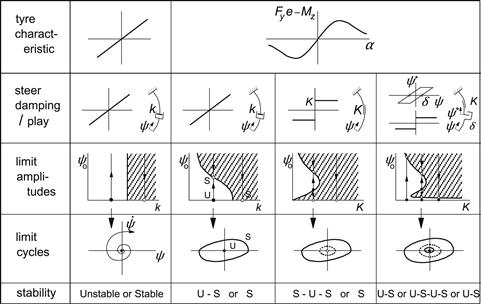
FIGURE 6.25 Linear and nonlinear systems considered and their autonomous motion properties in terms of stability and possible limit cycles.
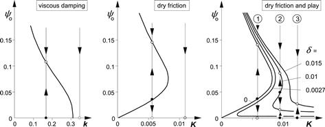
FIGURE 6.26 Limit amplitudes as a function of damping for increasing number of nonlinear elements: nonlinear tire, dry friction, and play (V = 6.66, σ = 3, e = 0, κ∗ = 0).
If dry friction is considered instead of the viscous damping, we observe that the center position is stable. In fact, the system may find its rest position away from the center (at a small steer angle) if the dry frictional torque is sufficiently large. We now need a finite external disturbance (running over an asymmetric obstacle) to overcome the dry friction. If that has happened, the motion develops itself further and the stable limit cycle is reached. If the initial conditions are chosen correctly we may spend a while near the unstable limit cycle before either the rest position or the large stable limit cycle is approached.Figure 6.27 shows for this case the solutions in the three-dimensional state space. The unstable limit cycle appears to lie on a tube-shaped surface which is here the separatrix in the solution space. We see that when the initial conditions are taken outside the tube, the stable limit cycle is reached. When the starting condition is inside the tube, one of the indicated possible rest positions will be ultimately attained.
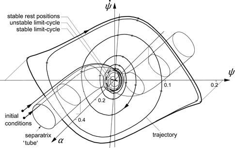
FIGURE 6.27 Solutions in the three-dimensional state space. System with nonlinear tire and dry friction (V = 6.66, σ = 3, e = 0, κ∗ = k = δ = 0, K = 0.0035). Line piece for possible rest positions, unstable and stable limit cycle. Tube-shaped separatrix separating space of trajectories leading to a rest position from the space of solution curves leading to the stable limit cycle.
The introduction of play about the steering axis, with δ being half the clearance space, appears indeed to be able to relax the action of the dry friction. For small play and enough dry friction (case 2 in Figure 6.26) the small stable limit cycle is reached automatically. An additional disturbance may cause the motion to get over the ‘nose’ and reach the large stable limit cycle. The plot of Figure 6.28 shows for this case the three limit cycles and trajectories as projected on the ![]() plane. If the play is larger or the damping less, the large limit cycle is reached without an external disturbance.
plane. If the play is larger or the damping less, the large limit cycle is reached without an external disturbance.
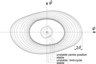
FIGURE 6.28 Limit cycles and trajectories for the system with nonlinear tire, dry friction, and play in the wheel bearings (Case 2 of Figure 6.26).
It is of interest to see how the limit amplitudes ψo vary with the speed of travel V. Figure 6.29 depicts two cases: viscous damping and dry friction. The area inside which the amplitude increases due to instability may be designated as the area of self-excitation. The diagrams show the courses of the limit amplitude for the two configurations with linear damping (K = δ = 0) with unstable ranges of speed indicated in Figure 6.3.
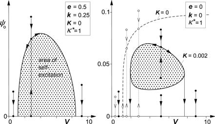
FIGURE 6.29 Boundary of area of self-excitation representing the course of limit amplitudes of steer angle ψ as a function of speed for system with nonlinear tire and viscous damping (left and right) and dry friction (right) (σ = 3, cf. Figure 6.3).
The right-hand diagram also gives the (smaller) area of self-excitation when dry friction is added. When the damping is linear, shimmy arises when the critical speed is exceeded. The amplitude grows as the vehicle speeds up. In the left-hand diagram, a maximum is reached beyond which the amplitude decreases and finally, at the higher boundary of stability, the oscillation dies out. With dry friction, the stable limit cycle cannot be reached automatically. A sufficiently strong external disturbance may get the shimmy started.
Another way of initiating the shimmy in the case of dry friction may be the application of wheel unbalance. Beyond a certain speed, the imposed unbalance couple may have become large enough to overcome the dry friction. Then, when the forcing frequency is not too much apart from the shimmy natural frequency, the amplitude rises quickly and a state of synchronous motion may arise as depicted in Figure 6.30. In that state, the system oscillates with a single frequency which corresponds to the wheel speed of revolution. When from that point onwards the vehicle speed is increased or decreased, the synchronous oscillation may persist until the difference between the two frequencies becomes too large (in other words, until the difference between free shimmy wavelength and wheel circumference is too great, that is, the system is detuned too much). Then, the unbalance torque is no longer able to drag the free shimmy motion along. The picture of the oscillation is now changed considerably. We have a motion with a beat character that consists of oscillations with two frequencies: one is the unbalance forcing frequency and the other will be close to the free shimmy frequency at the current speed. The shaded areas shown in the diagram indicate the speed ranges where these combination vibrations show up. The upper and lower boundaries of these areas represent the limits in between which the amplitude of the motion varies. When at decreasing speed the point at the vertical tangent to the area of self-excitation is reached, the shimmy oscillation disappears. At increasing speed, the combination oscillations may pass to a forced vibration with a single frequency. This occurs when the degree of self-excitation has become too low. A similar phenomenon of synchronous motions and combined oscillations has been treated by Stoker (1950, p.166). He uses an approximate analytical method to investigate the second-order nonlinear system of Van der Pol that is provided with a forcing member.
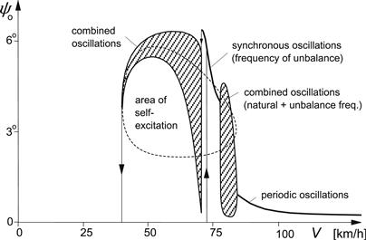
FIGURE 6.30 The response of the tenth-order system, representing a light truck with nonlinear tire and dry friction, to wheel unbalance moment. The area of self-excitation of the autonomous system has been indicated. At nearly 75 km/h violent shimmy develops. Then a range of speed with the so-called synchronous oscillations occurs. When the system is detuned too much, combined oscillations (beats) show up.
The diagram of Figure 6.30 represents the result of a computer simulation study with a relatively complex model of the 10th order. The model is developed to investigate the violent shimmy vibration generated by a light military truck equipped with independent trailing arm front-wheel suspensions. For details, we refer to the original publication, Pacejka (1966). The model features degrees of freedom represented by the following motion variables: lateral displacement and roll of the chassis, lateral and camber deflection of the suspension, steer angle of the front wheel (same left/right), rotation of the steering wheel, and lateral tire deflection. The degree of freedom of the steering wheel has been suppressed in the depicted case by clamping the steering system in the node that appears to occur in the free motion with the front wheels and the steering wheel moving in counter phase. The other lower frequency mode with front wheels and steering wheel moving in phase occurs at lower values of speed and partly overlaps the range of the counter-phase mode. It is expected that the in-phase mode is easily suppressed by loosely holding the steering wheel. This was more or less confirmed by experiments on a small mechanical wheel suspension/steering system model. The full-scale truck only showed shimmy with counter oscillating front wheels and steering wheel.
Finally, Figure 6.31 presents the results of measurements performed on the truck moving over a landing strip. The front wheels were provided with unbalance weights. Shimmy appeared to start at a speed of ca. 75 km/h. Synchronous oscillations were seen to occur as can be concluded by considering the frequencies that appear to coincide in the small range of speed just below the speed of initiation of 75 km/h. Further downwards, the frequencies get separated and follow independent courses. This strengthens the impression that here the motion may be able to sustain itself. Afterwards, another test was conducted with only one wheel provided with an unbalance weight. The weight was attached to a cable that made it possible to remove the unbalance during the test run. After having the unbalance detached at the instant that the shimmy was fully developed, the shimmy remained to manifest itself with about the same intensity. This constituted the proof that we dealt with a self-sustained oscillation. The correspondence between the diagrams of Figures 6.30 and 6.31 is striking. Also, the frequency of the autonomous vibration of the model (along the upper boundary of the area of self-excitation shown in Figure 6.30) was close to that according to the test results. The model frequency appears to vary from 6.1 Hz at the low end of the speed (40–45 km/h) to 7 Hz at the initiation velocity of 70–75 km/h.

FIGURE 6.31 Front wheel steer oscillation amplitude as a response to wheel unbalance as measured on a light truck. The speed is gradually reduced after violent shimmy was developed at ca. 75 km/h. After a short range of speed exhibiting synchronous oscillations (single frequency), combined vibrations occur with two distinct frequencies.