
Chapter 5
Non-Steady-State Out-of-Plane String-Based Tire Models
Chapter Outline
5.2. Review of Earlier Research
5.3. The Stretched String Model
5.4. Approximations and Other Models
Von Schlippe’s Straight Connection Model
Smiley’s and Roger’s Approximations
Straight Tangent Approximation
Approximations of Tread Width Moment Response
5.4.3. Enhanced String Model with Tread Elements
Non-Steady-State Behavior at Vanishing Sliding Range (Linear Analysis)
5.1 Introduction
The transient and oscillatory dynamic behavior of the tire will be discussed in this and two ensuing chapters. The present chapter is devoted to the model development of the tire as an integral component. The stretched string model is chosen as the basis for the physical description of the out-of-plane (anti-symmetric) behavior. This model exhibits a finite contact length that allows the study of short path wavelength phenomena. The model is relatively simple in structure and integrates the carcass compliance and contact patch slip properties. For the moment response to yaw variations, the finite width of the contact patch needs to be introduced which is accomplished by connecting to the string the brush model featuring only fore-and-aft tread element compliance. In the more advanced string model, the added tread elements are allowed to also deflect sideways. The behavior of this more complex model is expected to be more realistic. This becomes especially apparent in the treatment of the side force response to a constant slip angle when the wheel runs over an undulated road surface. The inertia of the tire is of importance when running at higher speeds (gyroscopic couple) and when the frequency of lateral and yaw excitation can no longer be considered small. Several approximations of the kinematic and dynamic model will be discussed. In Chapter 6, the theory will be applied in the analysis of the wheel shimmy phenomenon. In Chapter 7, the model will be simplified to the single-point contact model that restricts the application to longer wavelength situations but enables the extension of the application to longitudinal and combined transient slip situations. Chapter 9 treats the more complex model that includes an approximate representation of the effect of the finite contact length, the compliance of the carcass, and the inertia of the belt. This more versatile model is able to consider both out-of-plane and in-plane tire dynamic behavior that can be extended to the nonlinear slip range also at relatively short wavelengths. Moreover, rolling-over road unevennesses will be included in Chapter 10.
5.2 Review of Earlier Research
In the theories describing the horizontal non-steady-state behavior of tires, one can identify two trends of theoretical development. One group of authors assumes a bending stiffness of the carcass and the other bases its theory on the string concept.
In principle, the string theory is simpler than the beam theory, since with the string model the deflection of the foremost point alone determines the path of the tread for given wheel movements, whereas with the beam model the slope at the foremost point also has to be taken into account as an additional variable. The latter leads to an increase in the order of the system by one.
Von Schlippe (1941) presented his well-known theory of the kinematics of a rolling tire and introduced the concept of the stretched string model. For the first time, a finite contact length was considered. In the same paper, Dietr applied this theory to the shimmy problem. Later on, two papers of Von Schlippe and Dietrich (1942,1943) were published in which the effect of the width of the contact area is also considered. Two rigidly connected coaxial wheels, both approximated by a one-dimensional string model, are considered. The strings and their elastic supports are also supposed to be elastic in the circumferential direction.
Segel (1966) derived the frequency response characteristics for the one-dimensional string model. These appear to be similar to response curves which arise in Saito's approximate theory for the beam model (1962). For the same string model, Sharp and Jones (1980) developed a digital simulation technique which is capable of generating the exact response of the model. Earlier, Pacejka (1966) employed an analog computer and tape recorder (as a memory device) for the simulation according to the excellent von Schlippe approximation in which the contact line is approximated by a straight line connecting the two end points.
Smiley (1958) gave a summary theory resembling the one-dimensional theory of von Schlippe (1941). He has correlated various known theories with several systematic approximations to his summary theory.
Pacejka (1966) derived the non-steady-state response of the string model of finite width provided with tread elements. The important gyroscopic effect due to tire inertia has been introduced and the nonlinear behavior of the tire due to partial sliding has been discussed. Applications of the tire theory to the shimmy motion of automobiles were presented. In Pacejka (1972), the effect of mass of the tire has been investigated with the aid of an exact analysis of the behavior of a rolling stretched string tire model provided with mass. This complicated and cumbersome theory not suitable for dynamic vehicle studies was then followed by an approximate more convenient theory (Pacejka, 1973a), taking into account the inertial forces only up to the first harmonic of its distribution along the tire circumference. An outline of the theory together with experimental results will be given in the present chapter.
Rogers derived empirical differential equations (1971) which later were given a theoretical basis (1972). As a result of Rogers' research, shimmy response of tires in the low frequency range (mass effect not included!) can be described satisfactorily up to rather high reduced frequencies (i.e. short wavelengths) by using simple second-order differential equations.
Sperling (1977) conducted an extensive comparative study of different kinematic models of rolling elastic wheels. Recently, Besselink (2000) investigated and compared a number of interesting earlier models (Von Schlippe, Moreland, Smiley, Rogers, Kluiters, Keldysh, Pacejka) in terms of frequency response functions and step responses to side slip, path curvature (turn slip), and yaw angle, and judged their performances also in connection with the shimmy phenomenon.
Sekula et al. (1976) derived transfer functions from random slip angle input test data in the range of 0.05–4.0 Hz. From this information, cornering force responses were deduced for both radial and bias-ply tires to slip angle step inputs. Ho and Hall (1973) conducted an impressive experimental investigation using relatively small aircraft tires tested on a 120-inch research road wheel up to an oscillating yaw frequency of 3 Hz. A critical correlation study with theoretical results revealed that reasonable or good fit of the experimental frequency response plots can be achieved by using the theoretical functions (5.32, 5.92, 5.93) presented hereafter. It should be pointed out that in testing small-scale tires, certain similarity rules, cf. Pacejka (1974), should be obeyed.
Full-scale experimental tire frequency response tests have been carried out by several researchers, e.g., by Meier-Dörnberg, up to a yaw frequency of 20 Hz. Some of the latter investigations have been reported on by Strackerjan (1976). This researcher developed a dynamic tire model based on a somewhat different modeling philosophy compared to the model described by Pacejka (1973a) and discussed hereafter. Both types of models show good agreement with measured behavior. The straightforward approach employed by Strackerjan is similar to the method followed in Chapter 9.
In 1977, Fritz reported on an extensive experimental investigation concerning the radial force and the lateral force and aligning torque response to vertical axle oscilla at different constant yaw (side slip) angles of the wheel. Also, the mean values of the side force and of the moment have been determined. Earlier, Metcalf (1963) conducted small-scale tire experiments and Pacejka (1981) produced theoretical results in terms of mean cornering stiffness using a taught string tire model provided with elastic tread elements. Laerman (1986) conducted extensive tests on both car and truck tires and compared results with a theoretical model in terms of average side force and aligning torque and frequency response characteristics. The model includes tire mass (based on Strackerjan 1976) and allows sliding of tread elements with respect to the ground. Similar experiments on car tires have been carried out by Takahashi and Pacejka (1987). They developed a relatively simple mathematical model suitable for vehicle dynamics studies, including cornering on uneven roads (cf. Chapter 8).
In 2000 Maurice published experimental data up to over 60 Hz and a dynamic and short wavelength nonlinear model development that will be dealt with in Chapter 9. The model is connected with the in-plane dynamic model of Zegelaar (1998, cf. Chapter 9) and forms a versatile combined slip model that works with the Magic Formula steady-state functions presented in Chapter 4.
Another aspect of tire behavior is the non-steady-state response to wheel camber variations. Segel and Wilson (1976) found for a specific motorcycle tire that after a step change in camber angle about 20 percent of the ultimately attained side force responds instantaneously to this input. The remainder responds in a way similar to the response of the side force to a step change in slip angle, although with a larger relaxation length. Higuchi (1997) conducted comprehensive research on the nonlinear response to camber based on the string model and experimentally assessed responses to stepwise changes of the camber angle. In Chapter 7, the response to camber changes will be discussed.
The next section treats the essentials of the theory of lateral and yaw tire non-steady-state and dynamic behavior on the basis of the stretched string model.
5.3 The Stretched String Model
The tire model, depicted in Figure 5.1, consists of an (assumedly endless) string which is kept under a certain pretension by a uniform radial force distribution (comparable with inflation pressure in real tires). In the axial direction, the string is elastically supported with respect to the wheel-center-plane but is prevented from moving in the circumferential direction. The string contacts the horizontal smooth road over a finite length. It is assumed that the remaining free portion of the string maintains its circular shape (in side view).
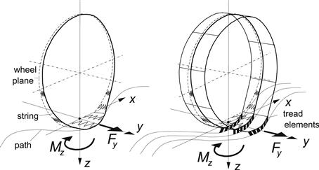
FIGURE 5.1 Tire model with single stretched string and model extended with more parallel strings provided with tread elements which are flexible in the longitudinal direction.
The model may be extended with a number of parallel strings keeping a constant mutual distance. As a result of this extension, a finite contact width arises. The strings are thought to be provided with a large number of elastic tread elements which, for reasons of simplification, are assumed to be flexible in the circumferential direction only. From the above assumptions, it follows that longitudinal deformations which arise at both sides of the wheel-center-plane when the wheel axle is subjected to a yaw rate are supposed to be taken up by the tread elements only.
For the theory to be linear, we must restrict ourselves to small lateral deformations and assume complete adhesion in the contact area. The wheel-center-plane is subjected to motions in the lateral direction (lateral displacement ![]() ) and about the axis normal to the road (yaw angle ψ). These motions constitute the input to the system. The excitation frequency is denoted by ω (=2πn). With V representing the assumed constant speed of travel, we obtain for the spatial or path frequency ωs = ω/V and the wavelength of the path of contact points λ = V/n = 2π/ωs. The distance traveled becomes s = Vt.
) and about the axis normal to the road (yaw angle ψ). These motions constitute the input to the system. The excitation frequency is denoted by ω (=2πn). With V representing the assumed constant speed of travel, we obtain for the spatial or path frequency ωs = ω/V and the wavelength of the path of contact points λ = V/n = 2π/ωs. The distance traveled becomes s = Vt.
Alternative input quantities may be considered which are not related to the position of the wheel with respect to the road but to its rate of change characterized by the slip angle ![]() and the path curvature or turn slip φ = −dψ/ds. The force Fy and the moment Mz which act from the ground on the tire in the y-direction and about the z-axis respectively form the response to the imposed wheel plane motion.
and the path curvature or turn slip φ = −dψ/ds. The force Fy and the moment Mz which act from the ground on the tire in the y-direction and about the z-axis respectively form the response to the imposed wheel plane motion.
5.3.1 Model Development
To obtain an expression for the lateral deflection v of the string, we consider the lateral equilibrium of an element of the tread band shown in Figure 5.2. The element is of full tread width and contains elements of the parallel strings with the rubber in between. In the lateral direction (y), the equilibrium of forces acting on the element of length dx and width 2b results in the following equation:
![]() (5.1)
(5.1)
where cc denotes the lateral carcass stiffness per unit length, S1 the circumferential (in the x-direction) component of the total tension force acting on the set of strings, and D the shear force in the cross section of the tread band acting on the rubber matrix. The shear force is assumed to be a linear function of the shear angle according to formula
![]() (5.2)
(5.2)

FIGURE 5.2 Lateral equilibrium of deflected tread band element.
With the introduction of the effective total tension S = S1 + S2, we deduce from Eqn (5.1)
![]() (5.3)
(5.3)
In the part of the tire not making contact with the road, the contact pressure vanishes so that qy = 0 and
![]() (5.4)
(5.4)
The lateral behavior of the model with several parallel strings and of the model with a single string will be identical if parameter S is the same. In Figure 5.3, a top view of the single string model is depicted. The length σ, designated as the relaxation length, has been indicated in the figure. The relaxation length equals:
![]() (5.5)
(5.5)
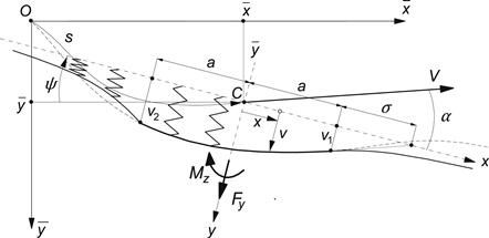
FIGURE 5.3 Top view of the single string model and its position with respect to the fixed frame.
With this quantity introduced, Eqn (5.4) for the free portion of the string becomes
![]() (5.6)
(5.6)
If we consider the circumference of the tire to be much longer than the contact length, we may assume that the deflection v2 at the trailing edge has a negligible effect on the deflection v1 at the leading edge. The deflections of the free string near the contact region may then be considered to be the result of the deflections of the string at the leading edge and at the trailing edge respectively and not of a combination of both. The deflections in these respective regions now read approximately:
![]() (5.7)
(5.7)
which constitute the solution of Eqn (5.6) considering the simplifying boundary condition that for large |x| the deflection tends to zero. At the edges x = ±a where v = v1 and v = v2 respectively, we have, for the slope,
 (5.8)
(5.8)
Because we do not consider the possibility of sliding in the contact zone, a kink may show up in the shape of the deflected string at the transition points from the free range to the contact zone. It seems a logical assumption that through the rolling process, the string forms a continuously varying slope around the leading edge while at the rear, because of the absence of bending stiffness, a discontinuity in slope may occur. An elegant proof of this statement follows by considering the observation that in vanishing regions of sliding at the transition points, cf. Figure 5.4, the directions of sliding speed of a point of the string with respect to the road and the friction force exerted by the road on the string that is needed to maintain a possible kink are compatible with each other at the trailing edge but incompatible at the leading edge. Therefore, it must be concluded that a kink may only arise at the trailing edge of the contact line. Consequently, the equation for the slope at the leading edge (first of (5.8)) can be rewritten as
![]() (5.9)
(5.9)
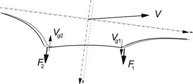
FIGURE 5.4 Two successive positions of the string model. Vanishing regions of sliding at the leading and trailing edges and the compatibility of sliding speed Vg and frictional forces F required to maintain a possible kink which apparently can only exist at the trailing edge (2).
This equation constitutes an important relationship for the development of the ultimate expression for the deflection of the string as we will see a little later.
In Chapter 2, we have derived the general differential equations for the longitudinal and lateral sliding velocity of a rolling body which is subjected to lateral slip and spin. These equations (2.58, 2.59) become, if the sliding speed equals zero as is our assumption here,
![]() (5.10)
(5.10)
![]() (5.11)
(5.11)
In these equations, s denotes the distance traveled by the wheel center (or better: the contact center) and x and y the coordinates the considered particle would have with respect to the moving axes system (C, x, y) in the horizontally undeformed state.
These partial differential equations will be solved by using Laplace transformation. The transforms will be written in capitals. The transformation will not be conducted with respect to time but with respect to the distance traveled s = Vt where the speed V is assumed to be a constant. The Laplace transform of a variable quantity, generally indicated by q, is defined through
![]() (5.12)
(5.12)
where p is the Laplace variable.
With initial conditions u(x, 0) = v(x, 0) = 0 at s = 0, we obtain, from (5.10, 5.11) the transformed equations,
![]() (5.13)
(5.13)
![]() (5.14)
(5.14)
The solutions of these ordinary first-order differential equations read
![]() (5.15)
(5.15)
![]() (5.16)
(5.16)
In Eqns (5.15, 5.16), the coefficients Cu and Cv are constants of integration. They are functions of p and depend on the tire construction, which is the structure of the model. For our string model with tread elements which can be deformed in the longitudinal direction only, we have the boundary conditions at the leading edge x = a:
![]() (5.17)
(5.17)
and
![]() (5.18)
(5.18)
with the latter Eqn (5.18) corresponding to Eqn (5.9).
The constant Cu now obviously becomes
![]() (5.19)
(5.19)
For the determination of Cv, we have to differentiate Eqn (5.16) with respect to x:
![]() (5.20)
(5.20)
With (5.18), we obtain
![]() (5.21)
(5.21)
which with (5.16) yields for the deflection at the leading edge
![]() (5.22)
(5.22)
and for the deflection in the contact zone
 (5.23)
The terms containing ep(x−a) point to a retardation behavior, which corresponds to delay terms in the original expressions. Note that a memory effect exists due to the fact that the nonsliding contact points retain information about their location with respect to the inertial system of axes ![]() as long as they are in the contact zone.
as long as they are in the contact zone.
Eqn (5.22) transformed back yields the first-order differential equation for the deflection of the string at the leading edge:
![]() (5.24)
(5.24)
This equation which is of fundamental importance for the transient behavior of the tire model (note the presence of the relaxation length σ in the left-hand member) might have been found more easily by considering a simple trailing wheel system with trail equal to σ and swivel axis located in the wheel plane a distance σ + a in front of the wheel axis, cf. Figure 5.3. The equation may also be found immediately from Eqn (5.14) by taking x = a and considering condition (5.9). Eqn (5.16) may also be transformed back which produces the delay terms mentioned before. However, we prefer to maintain the expression in the transformed state since we would like to obtain the result, that is: the force and moment response, in the form of transfer functions.
The Force and Moment Transfer Functions
For the calculation of the lateral force Fy and the moment ![]() due to lateral deflections acting on the string two methods may be employed. According to the first method used by von Schlippe and Dietrich (1941) and by Segel (1966), the internal (lateral) forces acting on the string are integrated along the length of the string extending from minus to plus infinity taking into account the circular shape of the string from side view. The latter is important for the moment acting about the vertical axis. A correct result for the moment is obtained if not only the lateral forces acting on the string are taken into account but also the radial forces (the air pressure) which arise due to the string tension and which act along lines out of the center plane due to the lateral deflection of the string. Surprisingly, a simpler configuration where the string lies in horizontal plane (without considering the circular shape) appears to produce the same result. This is proven by considering the second method.
due to lateral deflections acting on the string two methods may be employed. According to the first method used by von Schlippe and Dietrich (1941) and by Segel (1966), the internal (lateral) forces acting on the string are integrated along the length of the string extending from minus to plus infinity taking into account the circular shape of the string from side view. The latter is important for the moment acting about the vertical axis. A correct result for the moment is obtained if not only the lateral forces acting on the string are taken into account but also the radial forces (the air pressure) which arise due to the string tension and which act along lines out of the center plane due to the lateral deflection of the string. Surprisingly, a simpler configuration where the string lies in horizontal plane (without considering the circular shape) appears to produce the same result. This is proven by considering the second method.
The second method which has been used by Temple (cf. Hadekel 1952) is much simpler and leads to the same correct result. The equilibrium of only that portion of the string is considered which makes contact with the road surface. On this piece of string, the internal lateral forces, the string tension force, and the external forces, constituting the force Fy and the moment ![]() , are acting (cf. Figure 5.5).
, are acting (cf. Figure 5.5).
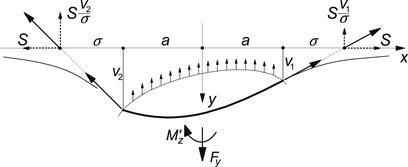
FIGURE 5.5 Equilibrium of forces in the contact region.
According to Temple's method, we obtain, for the lateral force,
![]() (5.25)
(5.25)
and, for the moment due to lateral deformations,
![]() (5.26)
(5.26)
with v1 and v2 denoting the deflections at x = a and −a respectively and S = σ2cc according to Eqn (5.5). For a first application of the theory, we refer to Exercise 5.1.
The moment ![]() due to longitudinal deformations which in our model are performed by only the tread elements is derived from the deflection u distributed over the contact area. With
due to longitudinal deformations which in our model are performed by only the tread elements is derived from the deflection u distributed over the contact area. With ![]() denoting the longitudinal stiffness of the elements per unit area, we obtain
denoting the longitudinal stiffness of the elements per unit area, we obtain
![]() (5.27)
(5.27)
By adding up both contributions, the total moment is formed:
![]() (5.28)
(5.28)
The Laplace transforms of Fy, ![]() , and
, and ![]() are now readily obtained using Eqns (5.23) and (5.15) with (5.19) and the transformed versions of Eqns (5.25), (5.26), and (5.27). In general, the transformed responses may be written as
are now readily obtained using Eqns (5.23) and (5.15) with (5.19) and the transformed versions of Eqns (5.25), (5.26), and (5.27). In general, the transformed responses may be written as
![]() (5.29)
(5.29)
etc. The coefficients of the transformed input variables constitute the transfer functions. The formulas, for convenience written in vectorial form, for the responses to α, φ, and ψ read (since ![]() expressions for the response to
expressions for the response to ![]() have been omitted)
have been omitted)
 (5.30)
 (5.31)
and furthermore
![]() (5.32)
(5.32)
in which the parameter
![]() (5.33)
(5.33)
has been introduced.
The transfer functions of the responses to ![]() and ψ are obtained by considering the relations between the transformed quantities
and ψ are obtained by considering the relations between the transformed quantities
![]() (5.34)
(5.34)
![]() (5.35)
(5.35)
and inserting these into (5.29). We find in general, for the transfer function conversion,
![]() (5.36)
(5.36)
![]() (5.37)
(5.37)
By transforming back the expressions such as (5.23, 5.29), the deflection, the force, and the moment can be found as a function of distance traveled s for a given variation of α and φ or of ![]() and ψ.
and ψ.
An interesting observation may be made when considering the situation depicted in Figure 5.6. Here a yaw oscillation of the wheel plane is considered around an imaginary vertical steering axis located at a distance σ + a in front of the wheel center. When yaw takes place about this particular point, the contact line remains straight and is positioned on the line along which the steering axis moves. Consequently, the response of the model to such a yaw motion is equal to the steady-state response. That is, for the force Fy and the moment ![]() , the transfer functions become equal to the cornering stiffness CFα and minus the aligning stiffness CMα respectively. As we realize that the angular motion about the σ + a point is composed of the yaw angle and the lateral displacement
, the transfer functions become equal to the cornering stiffness CFα and minus the aligning stiffness CMα respectively. As we realize that the angular motion about the σ + a point is composed of the yaw angle and the lateral displacement ![]() and furthermore that the response to
and furthermore that the response to ![]() is equal to the response to −α, we find, e.g., for the transfer function of Fy to ψσ+a,
is equal to the response to −α, we find, e.g., for the transfer function of Fy to ψσ+a,
![]() (5.38)
(5.38)
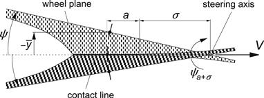
FIGURE 5.6 Steady-state response that occurs when swivelling about the σ + a point.
With the aid of (5.37), the fundamental relationship between the responses to α and φ can be assessed. We have, in general,
![]() (5.39)
(5.39)
where for the responses to Fy and ![]() we have the steady-state response functions denoted by Hψss:
we have the steady-state response functions denoted by Hψss:
![]() (5.40)
(5.40)
and
![]() (5.41)
(5.41)
The important conclusion is that we may suffice with establishing a single pair of transfer functions, e.g. Hα for Fy and ![]() , and derive from that the other functions by using the relations (5.36, 5.37, 5.39) together with (5.40, 5.41). Since in practice the frequency response functions are often assessed experimentally by performing yaw oscillation tests, we give below the conversion formulas to be derived from the transfer functions Hψ. Later on, we will address the problem of first subtracting
, and derive from that the other functions by using the relations (5.36, 5.37, 5.39) together with (5.40, 5.41). Since in practice the frequency response functions are often assessed experimentally by performing yaw oscillation tests, we give below the conversion formulas to be derived from the transfer functions Hψ. Later on, we will address the problem of first subtracting ![]() from the measured total moment Mz to retrieve
from the measured total moment Mz to retrieve ![]() for which the conversion is valid:
for which the conversion is valid:
![]() (5.42)
(5.42)
![]() (5.43)
(5.43)
![]() (5.44)
(5.44)
Strictly speaking, the above conversion formulas only hold exactly for our model. The actual tire may behave differently especially regarding the effect of the moment ![]() that in reality may slightly rotate the contact patch about the vertical axis and thus affects the slip angle seen by the contact patch. As a consequence, the observation depicted in Figure 5.6 may not be entirely true for the real tire.
that in reality may slightly rotate the contact patch about the vertical axis and thus affects the slip angle seen by the contact patch. As a consequence, the observation depicted in Figure 5.6 may not be entirely true for the real tire.
In the following, first the step response functions will be assessed and after that the frequency response functions.
5.3.2 Step and Steady-State Response of the String Model
An important characteristic aspect of transient tire behavior is the response of the lateral force to a stepwise variation of the slip angle α. The initial condition at s = 0 reads: v(x) = 0; for s > 0, the slip angle becomes α = αo. From Eqn (5.23), we obtain, for small slip angles by inverse transformation for the lateral deflection of the string in the contact region,
![]() (5.45)
(5.45)
while for the old points which are still on the straight contact line, the simple expression holds:
![]() (5.46)
(5.46)
Expression (5.45) is composed of a part (a − x)αo which is the lateral displacement of the wheel plane during the distance rolled a − x and an exponential part. The point which at the distance rolled s considered is located at coordinate x was the point at the leading edge when the wheel was rolled a distance a − x ago that is at s − a + x. At that instant, we had a deflection at the leading edge v1(s−a+x). The new v = v(s) equals the old v1 = v1(s−a+x) plus the subsequent lateral displacement of the wheel (a − x)αo. Obviously, the exponential part of (5.45) is the v1 at the distance rolled s − a + x. This can easily be verified by solving Eqn (5.24) for v1.
Finally, with (5.25) the expression for the force can be calculated for the two intervals, with and without the old contact points:
![]() (5.47)
(5.47)
![]() (5.48)
(5.48)
For the aligning torque, we obtain, by using (5.26),
![]() (5.49)
(5.49)
![]() (5.50)
(5.50)
where the quantities ![]() designate the unit step response functions. These functions correspond to the integral of the inverse Laplace transforms of the transfer functions (5.30, 5.31) given above.
designate the unit step response functions. These functions correspond to the integral of the inverse Laplace transforms of the transfer functions (5.30, 5.31) given above.
The graph of Figure 5.7 shows the resulting variation of Fy and ![]() vs traveled distance s. As has been indicated, the curves are composed of a parabola (of the second and third degree respectively) and an exponential function. The step responses have been presented as a ratio to their respective steady-state values.
vs traveled distance s. As has been indicated, the curves are composed of a parabola (of the second and third degree respectively) and an exponential function. The step responses have been presented as a ratio to their respective steady-state values.
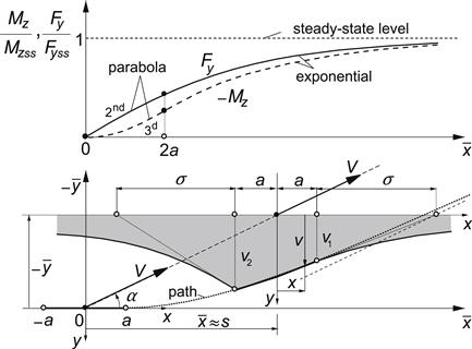
FIGURE 5.7 The response of the lateral force Fy and the aligning torque Mz to a step input of the slip angle α, calculated for a relaxation length σ = 3a.
The steady-state values of Fy and ![]() (or Mz) are directly obtained from (5.25) and (5.26) by considering the shape of the deflected string at steady-state side slip (Figure 5.8), i.e. a straight contact line at an angle α with the wheel plane and a deflection at the leading edge v1 = σα through which the condition to avoid a kink in the string at that point is obeyed, or from Eqns (5.48, 5.50) by letting s approach infinity. We have
(or Mz) are directly obtained from (5.25) and (5.26) by considering the shape of the deflected string at steady-state side slip (Figure 5.8), i.e. a straight contact line at an angle α with the wheel plane and a deflection at the leading edge v1 = σα through which the condition to avoid a kink in the string at that point is obeyed, or from Eqns (5.48, 5.50) by letting s approach infinity. We have
![]() (5.51)
(5.51)
![]() (5.52)
(5.52)
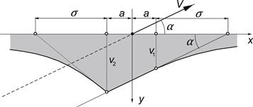
FIGURE 5.8 Steady-state deflection of a side slipping string tire model (complete adhesion).
with the cornering and aligning stiffnesses
![]() (5.53)
(5.53)
![]() (5.54)
(5.54)
and the pneumatic trail
![]() (5.55)
(5.55)
The variation of these quantities and of the pneumatic trail t = CMα/CFα and also of the relaxation length with wheel load Fz, the latter being assumed to vary proportionally with a2, turns out to be quite unrealistic when compared with experimental evidence. A variation much closer to reality would be obtained if tread elements were attached to the string. For more details, also concerning the nonlinear characteristics and the nonsteady analysis of that enhanced but much more complicated model, we refer to Section 5.4.3.
The unit step response functions ![]() to the other input variable φ and the associated variables
to the other input variable φ and the associated variables ![]() and ψ are of interest as well. They can be derived by integration of the unit impulse response functions Π(s), which are found by inverse transformation of the transfer functions (5.30, 5.31, 5.36, 5.37). Alternatively, the other step response functions may be directly established by considering the associated string deflections similar to (5.45, 5.46) or from the unit step responses to the slip angle, corresponding to the coefficients of α0 shown in (5.47–5.50), by making use of the following relationships analogous to Eqns (5.39, 5.36, 5.37):
and ψ are of interest as well. They can be derived by integration of the unit impulse response functions Π(s), which are found by inverse transformation of the transfer functions (5.30, 5.31, 5.36, 5.37). Alternatively, the other step response functions may be directly established by considering the associated string deflections similar to (5.45, 5.46) or from the unit step responses to the slip angle, corresponding to the coefficients of α0 shown in (5.47–5.50), by making use of the following relationships analogous to Eqns (5.39, 5.36, 5.37):
![]() (5.56)
(5.56)
![]() (5.57)
(5.57)
![]() (5.58)
(5.58)
Figure 5.9 illustrates the manner in which the deflection of the string model reacts to a step change of each of the four wheel motion variables (slip angle, lateral displacement of the wheel plane, turn slip, and yaw angle). Figure 5.10 presents the associated responses of the side force and the aligning torque. The responses have been divided by either the ultimate steady-state value of the transient response or the initial value, if relevant. For the moment response to turn slip and lateral displacement, both the initial and the final values vanish and a different reference value had to be chosen to make them nondimensional. The various steady-state coefficients and the lateral and torsional stiffnesses read in terms of the model parameters:
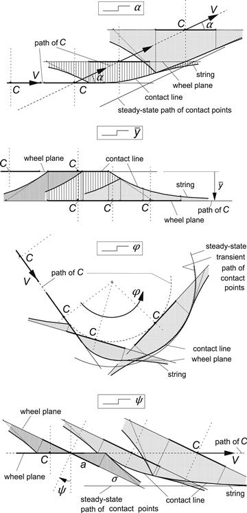
FIGURE 5.9 Transient response of string deflection to step change in motion variables.
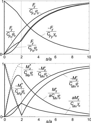
FIGURE 5.10 Unit step response of side force Fy, aligning torque ![]() and tread width moment
and tread width moment ![]() to slip angle α, lateral displacement
to slip angle α, lateral displacement ![]() , turn slip φ, and yaw angle ψ. Computed for string model with relaxation length σ = 3a.
, turn slip φ, and yaw angle ψ. Computed for string model with relaxation length σ = 3a.
Lateral stiffness of the standing tire:
![]() (5.59)
(5.59)
Cornering or lateral slip stiffness
![]() (5.60)
(5.60)
Aligning stiffness
![]() (5.61)
(5.61)
Torsional stiffness of (thin) standing tire
![]() (5.62)
(5.62)
Turn slip stiffness for the force
![]() (5.63)
(5.63)
Note that the steady-state response of ![]() to φ equals zero. The responses to side slip have already been presented in Figure 5.7. It now appears that the response of the side force Fy to turn slip φ is identical to the response of the aligning torque due to lateral deflections
to φ equals zero. The responses to side slip have already been presented in Figure 5.7. It now appears that the response of the side force Fy to turn slip φ is identical to the response of the aligning torque due to lateral deflections ![]() to α. This reciprocity property is also reflected by the equality of the slip stiffnesses given by (5.61, 5.63). It furthermore appears that the responses of Fy to ψ and φ and of
to α. This reciprocity property is also reflected by the equality of the slip stiffnesses given by (5.61, 5.63). It furthermore appears that the responses of Fy to ψ and φ and of ![]() to α tend to approach the steady-state condition at the same rate. This will be supported by the later finding that the corresponding frequency responses at low frequencies (large wavelengths) are similar. The frequency responses at short wavelengths are mainly governed by the step response behavior shortly after the step change has commenced. As appears from the graphs, at distances rolled smaller than the contact length large differences in transient behavior occur. As expected, the initial responses of Fy to
to α tend to approach the steady-state condition at the same rate. This will be supported by the later finding that the corresponding frequency responses at low frequencies (large wavelengths) are similar. The frequency responses at short wavelengths are mainly governed by the step response behavior shortly after the step change has commenced. As appears from the graphs, at distances rolled smaller than the contact length large differences in transient behavior occur. As expected, the initial responses of Fy to ![]() and of
and of ![]() to ψ are immediate and associated with the respective stiffnesses (5.59, 5.62).
to ψ are immediate and associated with the respective stiffnesses (5.59, 5.62).
The response of the moment ![]() due to tread width modeled with the brush model that deflects only in the longitudinal direction may be derived by considering the Laplace transform of the longitudinal deflection u according to Eqn (5.15) with (5.19). Through inverse transformation or simply by inspection of the development of this deflection while the element moves through the contact range, the following expressions are obtained:
due to tread width modeled with the brush model that deflects only in the longitudinal direction may be derived by considering the Laplace transform of the longitudinal deflection u according to Eqn (5.15) with (5.19). Through inverse transformation or simply by inspection of the development of this deflection while the element moves through the contact range, the following expressions are obtained:
![]() (5.64)
(5.64)
![]() (5.65)
(5.65)
By using Eqn (5.27), the following expressions for the step response of ![]() to φ result:
to φ result:
![]() (5.66a)
(5.66a)
![]() (5.66b)
(5.66b)
The graphical representation of these formulas is given in Figure 5.10. The slip stiffness and stiffness coefficients employed read
Turn slip stiffness for the moment, cf. (5.66b):
![]() (5.67a)
(5.67a)
Torsional stiffness of standing tire due to tread width, cf. (5.32) with p → ∞:
![]() (5.67b)
(5.67b)
Note that the steady-state response of ![]() to φ equals zero.
to φ equals zero.
As a result of a step change in turn slip, longitudinal slip at both sides of the contact patch occurs. The transient response extends only over a distance rolled equal to the contact length, at the end of which the steady-state response has been reached. As indicated in the graph, the approach curve has a parabolic shape. The response to a step change in yaw angle is immediate (like that of ![]() ) after which a decline occurs which for
) after which a decline occurs which for ![]() is linear (derivative of response to φ).
is linear (derivative of response to φ).
In Figures 5.11 and 5.12, experimentally obtained responses to small step changes of the input have been presented. The diagrams show very well the exponential nature of the force response to side slip. Especially the aircraft tire exhibits the ‘delayed’ response of the aligning torque to side slip as predicted by the theory (Figure 5.10). Figure 5.12 shows a similar delay in the responses of Fy to turn slip also found in the theoretical results. The peculiar response of the moment to yaw and turn slip is clearly formed by the sum of the responses of ![]() and of
and of ![]() , although their ratio differs from the assumption adopted in Figure 5.10.
, although their ratio differs from the assumption adopted in Figure 5.10.
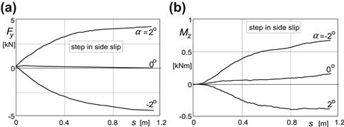
FIGURE 5.11 Step response of side force Fy and aligning torque Mz to slip angle α as measured on an aircraft tire with vertical load Fz = 35 kN.
(From Besselink 2000; test data is provided by Michelin Aircraft Tire Corporation).
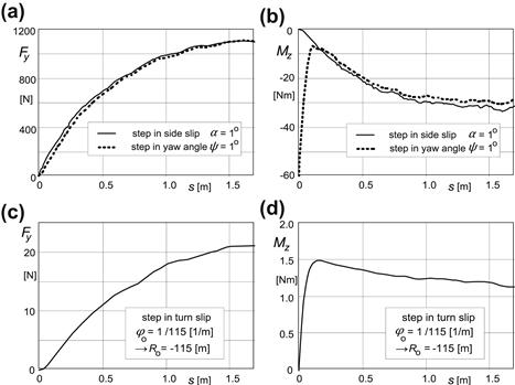
FIGURE 5.12 Step response of side force Fy and aligning torque Mz to slip angle α, yaw angle ψ, and turn slip φ (α = 0) as measured on a passenger car tire at load Fz = 4 kN. Tests were conducted on the flat plank machine of TU-Delft, cf. Figure 12.6 (Higuchi 1997, p. 44).
The response to a small step change in turn slip φo = −1/Ro has been obtained by integration of the response to a small turn slip impulse = − step yaw angle ψo (while α remains zero) and division by Ro ψo:
![]() (5.68a)
(5.68a)
![]() (5.68b)
(5.68b)
For ψo = −0.5° = −1/115 rad and by choosing Ro = 115 m, we divide by unity. For more details, we refer to Pacejka (2004).
Graphs of step response functions may serve to compare the performance of different models and approximations with each other. This will be done in Section 5.4. First we will discuss the frequency response functions.
5.3.3 Frequency Response Functions of the String Model
The frequency response functions for the force and the moment constitute the response to sinusoidal motions of the wheel and can be easily obtained by replacing in the transfer functions (5.30, 5.31, 5.32) the Laplace variable p byiωs. The path frequency ωs (rad/m) is equal to 2π/λ, where λ denotes the wavelength of the sinusoidal motion of the wheel. Figure 5.13 illustrates the manner in which the string deflection varies with traveled distance when the model is subjected to a yaw oscillation with different wavelengths.
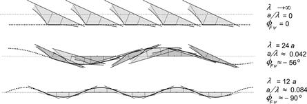
FIGURE 5.13 The string model at steady-state side slip and subjected to yaw oscillations with two different wavelengths λ.
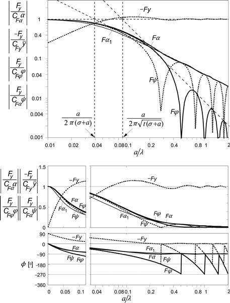
FIGURE 5.14 String model frequency response functions for the side force with respect to various motion input variables. The nondimensional path frequency is equal to half the contact length divided by the wavelength of the motion: a/λ = ωs/2π. For the response to α a first-order approximation with the same cutoff frequency, ωs = 1/(σ + a), has been added (Fα1). Three ways of presentation have been used: log–log, lin–log, and lin–lin. The model parameter σ = 3a, which leads to t = 0.77a.
The frequency response functions such as HF,ψ(iωs) are the complex ratios of output, e.g. Fy, and input, e.g. ψ. In Figures 5.14 and 5.15, the various frequency response functions have been plotted as a function of the nondimensional path frequency a/λ = ½ωsa/π. The functions are represented by their absolute value |H| and the phase angle ϕ of the output with respect to the input (if negative then output lags behind input), e.g.
![]() (5.69)
(5.69)
If the variables are considered as real quantities, one gets α = |α| cos(ωss) and, for its response, Fy = |Fy| cos(ωss + ϕ). In the figure, the absolute values have been made nondimensional by showing the ratio to their values at ωs = 0, the steady-state condition. Three different ways of presentation have been used, each with its own advantage.
The force response to slip angle very much resembles a first-order system behavior, as can be seen in the upper graph with a log–log scale. The cutoff frequency that is found by considering the steady-state response and the asymptotic behavior at large path frequencies appears to be equal to
![]() (5.70)
(5.70)
However, the phase lag at frequencies tending to zero is not equal to ωs(σ + a), as one would expect for a first-order system, but somewhat smaller. Analysis reveals that the phase lag tends to
![]() (5.71)
(5.71)
with the relaxation length for the side force with respect to the slip angle
![]() (5.72)
(5.72)
which with (5.55) becomes equal to 3.23a if σ = 3a. The phase lag does approach 90° for frequencies going to infinity. The first-order approximation with the same cutoff frequency has been added in the graph for comparison. The corresponding frequency response function reads
![]() (5.73)
(5.73)
The frequency response of the force to yaw shows a wavy curve for the amplitude at higher frequencies (at wavelengths smaller than ca. two times the contact length). The decline of the peaks occurs according to the same asymptote as found for the slip angle response. Consequently, the same cutoff frequency applies:
![]() (5.74)
(5.74)
When analyzing the behavior at small frequencies, it appears that here the phase lag does tend to
![]() (5.75)
(5.75)
with the relaxation length for the side force with respect to the yaw angle:
![]() (5.76)
(5.76)
Further analysis reveals that, when developing the frequency response function HF,ψ in a series up to the second degree in iωs,
![]() (5.77)
(5.77)
and subsequently employing the fundamental relationship (5.42) between α and φ responses, the frequency response function HF,α up to the first degree in iωs becomes
![]() (5.78)
(5.78)
which shows that
![]() (5.79)
(5.79)
which is an important result in view of assessing σFα from yaw oscillation measurement data and checking the correspondence with (5.72).
The aligning torque (![]() , Figure 5.15) shows a response to the slip angle which is closer to a second-order system with a phase lag tending to a variation around 180° and a 2:1 asymptotic slope of the amplitude with a cutoff frequency equal to
, Figure 5.15) shows a response to the slip angle which is closer to a second-order system with a phase lag tending to a variation around 180° and a 2:1 asymptotic slope of the amplitude with a cutoff frequency equal to
![]() (5.80)
(5.80)
where t denotes the pneumatic trail, cf. (5.55). Again, the response of Fy to φ turns out to be the same as the response of ![]() to α. As the graph of Figure 5.15 shows, the amplitude of
to α. As the graph of Figure 5.15 shows, the amplitude of ![]() as a response to yaw oscillations ψ exhibits a clear dip at (with parameter σ = 3a) a wavelength λ = ∼12a. This condition corresponds to the situation depicted in Figure 5.13 (third case) and is referred to as the meandering phenomenon or as kinematic shimmy which occurs in practice when the wheel is allowed to swivel freely about the vertical axis through the wheel center and the system is slowly moved forward. The nearly symmetric string deformation explains why the amplitude of the aligning torque almost vanishes at this wavelength. At higher frequencies, the amplitude remains finite and approaches at ωs → ∞ the same value as it had at ωs = 0 that is:
as a response to yaw oscillations ψ exhibits a clear dip at (with parameter σ = 3a) a wavelength λ = ∼12a. This condition corresponds to the situation depicted in Figure 5.13 (third case) and is referred to as the meandering phenomenon or as kinematic shimmy which occurs in practice when the wheel is allowed to swivel freely about the vertical axis through the wheel center and the system is slowly moved forward. The nearly symmetric string deformation explains why the amplitude of the aligning torque almost vanishes at this wavelength. At higher frequencies, the amplitude remains finite and approaches at ωs → ∞ the same value as it had at ωs = 0 that is: ![]() . The phase angle approaches −360°. It is interesting that analysis at frequencies approaching zero shows that the phase lag both for the response of
. The phase angle approaches −360°. It is interesting that analysis at frequencies approaching zero shows that the phase lag both for the response of ![]() to α and to ψ (and thus also for Fy to φ) approaches the value ωs (σ + a) that also appeared to be true for the response of Fy to ψ. So we have
to α and to ψ (and thus also for Fy to φ) approaches the value ωs (σ + a) that also appeared to be true for the response of Fy to ψ. So we have
![]() (5.81)
(5.81)
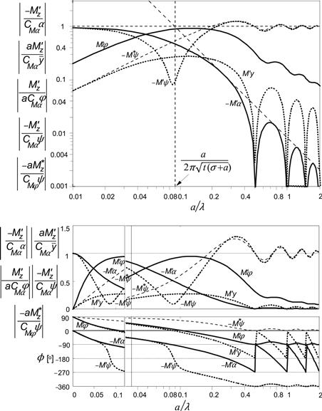
FIGURE 5.15 String model frequency response functions for the aligning torque with respect to various motion input variables. Same conditions as in Figure 5.14. The response functions of the moment due to tread width ![]() have been added.
have been added.
Expressions equivalent to (5.70, 5.72, 5.74, 5.79–5.81) appear to hold for the enhanced model with tread elements attached to the string, cf. Section 5.4.3.
The torque due to tread width ![]() shows a response to yaw angle ψ that increases in amplitude with path frequency and starts out with a phase lead of 90° with respect to ψ. At low frequencies, the moment acts like the torque of a viscous rotary damper with damping rate inversely proportional with the speed of travel V. We find, with Eqn (5.67),
shows a response to yaw angle ψ that increases in amplitude with path frequency and starts out with a phase lead of 90° with respect to ψ. At low frequencies, the moment acts like the torque of a viscous rotary damper with damping rate inversely proportional with the speed of travel V. We find, with Eqn (5.67),
![]() (5.82)
(5.82)
At high frequencies ωs → ∞, that is at vanishing wavelength λ → 0 where the tire is standing still, the tire acts like a torsional spring and the moment ![]() approaches
approaches ![]() , cf. (5.68). The cutoff frequency appears to become
, cf. (5.68). The cutoff frequency appears to become
![]() (5.83)
(5.83)
The total moment about the vertical axis is obtained by adding the components due to lateral and longitudinal deformations:
![]() (5.84)
(5.84)
For the standing tire, one finds from a yaw test the total torsional stiffness CMψ which relates to the aligning stiffness and the stiffness due to tread width as follows:
![]() (5.85)
(5.85)
Obviously, this relationship offers a possibility to assess the turn slip stiffness for the moment CMφ.
Due to the action of ![]() , the phase lag of
, the phase lag of ![]() will be reduced. This appears to be important for the stabilization of wheel shimmy oscillations (cf. Chapter 6). The total moment and its components can best be presented in a Nyquist plot where the moment components and the resulting total moment appear as vectors in a polar diagram. Figure 5.16 depicts the vector diagram at a low value of the path frequency ωs.
will be reduced. This appears to be important for the stabilization of wheel shimmy oscillations (cf. Chapter 6). The total moment and its components can best be presented in a Nyquist plot where the moment components and the resulting total moment appear as vectors in a polar diagram. Figure 5.16 depicts the vector diagram at a low value of the path frequency ωs.
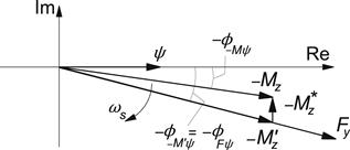
FIGURE 5.16 Complex representation of side force and moment response to yaw oscillations ψ.
By considering the various phase angles at low frequencies, we may be able to extract the moment response due to tread width from the total (measured) response and find the response of the moment for a ‘thin’ tire. Since at low frequencies the moment vector ![]() tends to point upward, we find, while considering (5.75, 5.81) and (5.82),
tends to point upward, we find, while considering (5.75, 5.81) and (5.82),
![]() (5.86)
(5.86)
With known σFψ and ϕ−Mψ to be determined from the measurement at low frequency, the moment turn slip stiffness CMφ = κ∗ may be assessed in this way.
In the diagrams of Figures 5.17 and 5.18, the nondimensional frequency response functions HF,ψ(iωs)/CFα and −HM,ψ(iωs)/CMα with its components ![]() and
and ![]() have been presented as a function of the nondimensional path frequency a/λ. The parameter values are σ = 3a and CMφ = aCMα.
have been presented as a function of the nondimensional path frequency a/λ. The parameter values are σ = 3a and CMφ = aCMα.
The diagram of Figure 5.17 clearly shows the increase in phase lag and decrease of the amplitude of Fy with decreasing wavelength λ. The wavy behavior and the associated jumps from 180° to 0 of the phase angle displayed in Figure 5.14 become clear when viewing the loops that appear to occur when the wavelength becomes smaller than about two times the contact length.
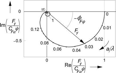
FIGURE 5.17 Nyquist plot of the nondimensional frequency response function of the side force Fy with respect to the wheel yaw angle ψ. Parameter: σ = 3a.
The aligning torque vector, Figure 5.18, for the ‘thin’ tire turns over 360° before from a wavelength of about the contact length the loops begin to show up. At about λ = 12a, the curve gets closest to the origin. This corresponds to the frequency where the dip occurs in Figure 5.15 and is illustrated as the last case of Figure 5.13.

FIGURE 5.18 Nyquist plot of the nondimensional frequency response function of the aligning moment Mz with respect to the wheel yaw angle ψ. The contributing components ![]() due to lateral deformations and
due to lateral deformations and ![]() due to tread width and associated longitudinal deformations. Parameters: σ = 3a and CMφ = aCMα .
due to tread width and associated longitudinal deformations. Parameters: σ = 3a and CMφ = aCMα .
For values of ![]() ∗ sufficiently large, the total moment curve does not circle around the origin anymore. The curve stretches more to the right and ends where the wheel does not roll anymore and the tire acts as a torsional spring with stiffness expressed by (5.85). In reality, the tire will exhibit some damping due to hysteresis. That will result in an end point located somewhat above the horizontal axis.
∗ sufficiently large, the total moment curve does not circle around the origin anymore. The curve stretches more to the right and ends where the wheel does not roll anymore and the tire acts as a torsional spring with stiffness expressed by (5.85). In reality, the tire will exhibit some damping due to hysteresis. That will result in an end point located somewhat above the horizontal axis.
The calculated behavior of the linear tire model has unmistakable points of agreement with results found experimentally at low values of the yaw frequency. At higher frequencies and higher speeds of rolling, the influence of the tire inertia and especially the gyroscopic couple due to tire lateral deformation rates is no longer negligible. In Section 5.5 and Chapter 9, these matters will be addressed.
Exercise 5.1. String Model at Steady Turn Slip
Consider the single stretched string tire model running along a circular path with radius R anti-clockwise (φ = 1/R) and without side slip (α = 0) as depicted in Figure 5.19.
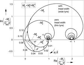
FIGURE 5.19 The string tire model in steady turning state (Ex. 5.1).
Derive the expression for the lateral force Fy acting upon the model under these steady-state circumstances. First find the expression for the lateral deflection v(x) using Eqn (2.61) which leads to a quadratic approximation of the contact line. Then use Eqn (5.25) for the calculation of the side force.
Now consider in addition some side slip and determine the value of α required to neutralize the side force generated by the path curvature 1/R. Make a sketch of the resulting string deformation and wheel-plane orientation with respect to the circular path for the following values of radius and relaxation length: R = 6a and σ = 2a.
5.4 Approximations and Other Models
In the present section, approximations to the exact theory will be treated to make the theory more accessible to applications. Subsection 5.4.2 discusses a number of other models known in the literature. After that in Subsection 5.4.3, a more complex model showing tread elements flexible also in the lateral direction will be treated to provide a reference model that is closer in performance to the real tire.
5.4.1 Approximate Models
In the literature, several simpler models have been proposed. Not all of these are based on the string model but many are. Figure 5.20 depicts a number of approximated contact lines as proposed by several authors. The most well-known and accurate approximation is that of Von Schlippe (1941) who approximated the contact line by forming a straight connection between the leading and trailing edges of the exact contact line. Kluiters (1969) gave a further approximation by introducing a Padé filter to approximately determine the location of the trailing edge. Smiley (1957) proposes an alternative approximation by considering a straight contact line that touches the exact contact line in its center in a more or less approximate way. Pacejka (1966) considered a linear or quadratic approximation of the contact line touching the exact one at the leading edge; the first and simplest approximation is referred to as the straight tangent approximation. A further simplification, completely disregarding the influence of the length of the contact line, results in the first-order approximation referred to as the point contact approximation.
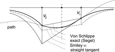
FIGURE 5.20 Several approximative shapes of the contact line of the string model.
In the sequel, we will discuss Von Schlippe's and Smiley's second-order approximation as well as the straight tangent and point contact approximations. The performance of these models will be shown in comparison with the exact ‘bare’ string model and with the enhanced model with laterally compliant tread elements. Figures 5.21–5.27 give the results in terms of step response, frequency response Bode plots, and Nyquist diagrams.
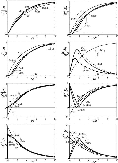
FIGURE 5.21 Step responses of side force and aligning torque to several inputs for exact and approximate models: ex.: exact ‘bare’ string model; vSch.: Von Schlippe; Sm2: Smiley second order; s.t.: straight tangent; a0: point contact; ex.tr.el.: exact with tread elements.
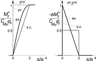
FIGURE 5.22 Step response of the moment due to tread width to turn slip (path curvature) and yaw angle for exact and approximations: ex.: exact (brush model); s.c.: straight connection (linear interpolation); 2nd: second-order approximation; 1st: first-order approximation.
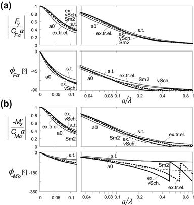
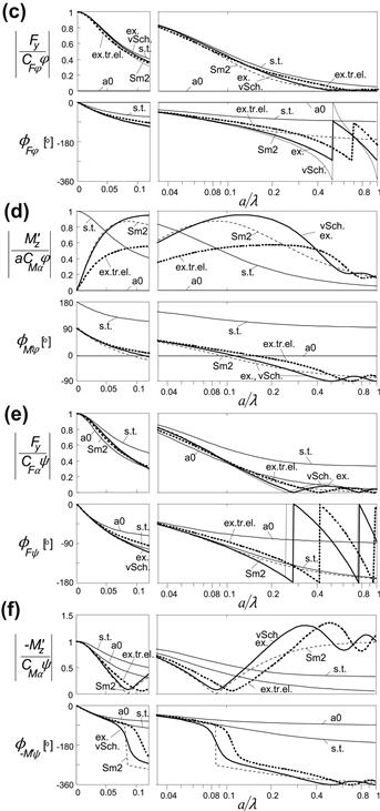
FIGURE 5.23 a,b,c,d,e,f. Frequency response functions of side force and aligning torque to several inputs for exact and approximate models: ex.: exact ‘bare’ string model; vSch.: Von Schlippe; Sm2: Smiley second order; s.t.: straight tangent; a0: point contact; ex.tr.el.: exact with tread elements.
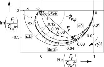
FIGURE 5.24 Nyquist plot of the frequency response function of the side force Fy with respect to the wheel yaw angle ψ. Parameter: σ = 3a. ex.: exact ‘bare’ string model; vSch.: Von Schlippe; Sm2: Smiley second order; s.t.: straight tangent; a0: point contact; ex.tr.el.: exact with tread elements.
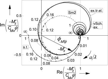
FIGURE 5.25 Nyquist plot of the frequency response function of the aligning torque − ![]() with respect to the wheel yaw angle ψ. Curve a0 is hidden by Sm2. Same conditions as in Figure 5.24.
with respect to the wheel yaw angle ψ. Curve a0 is hidden by Sm2. Same conditions as in Figure 5.24.
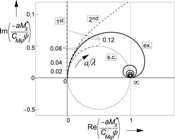
FIGURE 5.26 Nyquist plot of the frequency response function of the torque due to tread width ![]() with respect to the wheel yaw angle ψ. ex.: exact (brush); s.c.: straight connection (linear interpolation); 2nd: second-order app.; 1st: first-order approx.
with respect to the wheel yaw angle ψ. ex.: exact (brush); s.c.: straight connection (linear interpolation); 2nd: second-order app.; 1st: first-order approx.
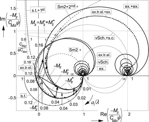
FIGURE 5.27 Nyquist plot of the nondimensional frequency response function of the aligning moment Mz with respect to the wheel yaw angle ψ. Contributing components ![]() due to lateral deformations and
due to lateral deformations and ![]() due to tread width and associated longitudinal deformations. Parameters: σ = 3a and CMφ = aCMα. Exact and approximate models: ex.: exact ‘bare’ string model; vSch.: Von Schlippe; Sm2: Smiley second order; s.t.: straight tangent; a0: point contact (hidden by Sm2); ex.tr.el.: exact with tread elements; ex.: exact (brush ); s.c.: straight connection (linear interpolation); 2nd : second-order approximation; 1st : first-order approx. (also CMφ = 0.6aCMα).
due to tread width and associated longitudinal deformations. Parameters: σ = 3a and CMφ = aCMα. Exact and approximate models: ex.: exact ‘bare’ string model; vSch.: Von Schlippe; Sm2: Smiley second order; s.t.: straight tangent; a0: point contact (hidden by Sm2); ex.tr.el.: exact with tread elements; ex.: exact (brush ); s.c.: straight connection (linear interpolation); 2nd : second-order approximation; 1st : first-order approx. (also CMφ = 0.6aCMα).
For some of the other approximate models (Rogers 1972, Kluiters 1969, Keldysh 1945 and Moreland 1954), only the governing equations will be provided with some comments on their behavior. For more information, we refer to the original publications or to the extensive comparative study of Besselink (2000).
The simplest models – straight tangent and point contact – can easily be extended into the nonlinear regime. In Chapter 6, this will be demonstrated for the straight tangent model in connection with the nonlinear analysis of the shimmy phenomenon. In Chapter 7, the nonlinear single-point contact model will be fully exploited. These models only show an acceptable accuracy for wheel oscillations at wavelengths which are relatively large with respect to the contact length. Chapter 9 is especially devoted to the development of a model that can operate at smaller wavelengths and nonlinear (combined slip) conditions which requires the inclusion of the effect of the length of the contact zone.
Von Schlippe's Straight Connection Model
This model which shows results that can hardly be distinguished from the exact ones only requires the string deflections at the leading and trailing edges v1 and v2. We find, for the Laplace transforms of these deflections as derived from the expressions (5.22, 5.23) in vectorial form,
![]() (5.87)
(5.87)
![]() (5.88)
(5.88)
where the exponential function refers to the retardation effect over a distance equal to the contact length. The transfer functions to the alternative set of input variables (y, ψ) may be obtained by using the conversion formulas (5.36, 5.37).
The responses to a step change in slip angle become, cf. (5.45, 5.46),
![]() (5.89)
(5.89)
![]() (5.90)
(5.90)
![]() (5.91)
(5.91)
Responses to step changes of other input variables may be determined by using the conversion formulas (5.56–5.58).
The side force and the aligning torque are obtained as follows:
![]() (5.92)
(5.92)
![]() (5.93)
(5.93)
The first equation shows that the force is obtained by multiplying the average lateral deflection with the lateral stiffness, cf. (5.59) with (5.60), and the moment by multiplying the slope of the connection line with the torsional stiffness of the ‘thin’ tire (5.62) or (5.61). It may be noted that due to the adopted straight contact line, the turn slip stiffness for the force becomes slightly less than the exact one (5.63):
![]() (5.94)
(5.94)
The various diagrams show that only in some particular cases, a (small) difference between ‘exact’ and ‘Von Schlippe’ can be observed. The model can be easily used in vehicle simulation studies by remembering the ![]() coordinates of the leading edge with respect to the global axis system (cf. Figure 5.3) and use these coordinates again after the wheel is rolled a distance 2a further when the trailing edge has assumed this location.
coordinates of the leading edge with respect to the global axis system (cf. Figure 5.3) and use these coordinates again after the wheel is rolled a distance 2a further when the trailing edge has assumed this location.
Smiley's and Roger's Approximations
Assuming in Figure 5.3 that the wheel moves along the ![]() axis with only small deviations in the lateral direction and in yaw, the lateral coordinate
axis with only small deviations in the lateral direction and in yaw, the lateral coordinate ![]() of the leading edge follows from Eqn (5.24). After realizing that
of the leading edge follows from Eqn (5.24). After realizing that
![]() (5.95)
(5.95)
the differential equation for ![]() becomes
becomes
![]() (5.96)
(5.96)
The problem Smiley has addressed is the assessment of the location of the center of the contact line. The lateral coordinate ![]() of this point may be approximated by using a Taylor series. Starting out from the position of the center contact point, the slope and the curvature etc. of the path of contact points, the relationship between the lateral coordinate of the foremost contact point and that of the center point can be written as follows:
of this point may be approximated by using a Taylor series. Starting out from the position of the center contact point, the slope and the curvature etc. of the path of contact points, the relationship between the lateral coordinate of the foremost contact point and that of the center point can be written as follows:
![]() (5.97)
(5.97)
Its derivative becomes
![]() (5.98)
(5.98)
After substitution of these series in Eqn (5.96), the following generic formula is obtained:
![]() (5.99)
(5.99)
The side force and the aligning torque can be found by multiplying the lateral deflection ![]() and the torsion angle
and the torsion angle ![]() with the respective stiffnesses CFy and
with the respective stiffnesses CFy and ![]() , cf. Eqns (5.59, 5.62). We obtain
, cf. Eqns (5.59, 5.62). We obtain
![]() (5.100)
(5.100)
![]() (5.101)
(5.101)
Using the conversion formulas (5.36, 5.37), the transfer functions with respect to α and φ can be obtained. For the order n of (5.99) equal to 2, the model becomes of the second order and one finds the following transfer functions in vector form:
 (5.102)
and
 (5.103)
It may be noted that the side force turn slip stiffness for this approximate model is somewhat larger than according to the exact expression. We have, for Smiley's model,
![]() (5.104)
(5.104)
The step responses of Figure 5.21 show reasonable to very good correspondence for the different inputs. Also, the frequency response functions, shown in Figure 5.23, indicate that the accuracy of this relatively simple Smiley2 approximation is quite good. The dip in the ![]() response to ψ is well represented and is located at the ‘meandering’ path frequency (zero of (5.103))
response to ψ is well represented and is located at the ‘meandering’ path frequency (zero of (5.103)) ![]() . The approximation may be considered to be acceptable for wavelengths larger than about 4 times the contact length (a/λ = 0.125). In his publication, Smiley recommends to use the order n = 3.
. The approximation may be considered to be acceptable for wavelengths larger than about 4 times the contact length (a/λ = 0.125). In his publication, Smiley recommends to use the order n = 3.
The initial empirically assessed formulas of Rogers (1972) are almost the same as the functions (5.102, 5.103); the terms ½a do not appear in his expressions but in the numerator of the moment response to turn slip (second element of 5.103) the empirically assessed term −ε is added. Also, a connection with Kluiters' approximation appears to exist.
Kluiters' Approximation
Kluiters (1969) (cf. Besselink 2000) adopted a Padé filter to approximate the position of the trailing edge. The transfer function of y2 with respect to y1 reads, if the order of the filter is taken equal to 2,
 (5.105)
with
![]() (5.106)
(5.106)
![]() (5.107)
(5.107)
We obtain, with (5.87),
 (5.108)
The deflection at the foremost point is, of course, governed by transfer function (5.87). The correspondence of this third-order model with Von Schlippe's model is very good for wavelengths larger than about 1.5 times the contact length. The accuracy is better than even Smiley's third-order approach. It turns out that when a first-order Padé filter is used, the formulas of Rogers without ε arise.
Straight Tangent Approximation
For this very simple approximation, the contact line is solely governed by the deflection v1 at the leading edge. The approximated shape of the deflected string corresponds to the steady-state deflection depicted in Figure 5.8 with deflection angle α′ = v1/σ. The side force and aligning torque are found by multiplying the deflection angle with the cornering stiffness and the aligning stiffness, respectively.
Using (5.87), we obtain, for the transfer functions,
![]() (5.109)
(5.109)
![]() (5.110)
(5.110)
The step responses equal the respective slip stiffnesses multiplied with the responses of v1/σ according to (5.89). As expected, the accuracy becomes much less and from the frequency response functions we may conclude that acceptable agreement is attained when the path frequency is limited to about a/λ = 0.04 or a wavelength larger than about 12 times the contact length. The response of the aligning torque to path curvature appears to be far off when compared with the exact responses. Since this particular response is the least important in realistic situations, the straight tangent model may still be acceptable. In the analysis of the shimmy phenomenon, this will be demonstrated to be true for speeds of travel which are not too low (where the wavelength becomes too short).
Figures 5.24 and 5.25 clearly show that at least up to a/λ = 0.04, the phase lag closely follows the exact variation with frequency. The amplitude, however, is too large, especially for the moment. A combination with a fictive ![]() (first-order approximation, see further on) with properly chosen parameter
(first-order approximation, see further on) with properly chosen parameter ![]() may help to reduce the amplitude of the moment to a more acceptable level also for nondimensional path frequencies higher than 0.04. Figure 5.27 shows a considerable improvement if we would choose CMφ = 0.6CMα.
may help to reduce the amplitude of the moment to a more acceptable level also for nondimensional path frequencies higher than 0.04. Figure 5.27 shows a considerable improvement if we would choose CMφ = 0.6CMα.
Differential Eqn (5.125), to be shown later on, governs the straight tangent approximation. Because we have a deflection shape equal to that occurring at steady-state side-slip motion, the extension of the model to nonlinear large slip conditions is easy to establish. We may employ the steady-state characteristics, e.g. Magic Formulas, and obtain
![]() (5.111)
(5.111)
with the deflection angle
![]() (5.112)
(5.112)
The amplitude of the self-excited shimmy oscillation appears to become limited due to the nonlinear, degressive, characteristics of the side force and the aligning torque versus slip angle.
Single-point Contact Model
This simplest approximation disregards the influence of the length of the contact line. The lateral deflection at the contact center at steady-state side slip should be taken equal to that of the exact model. This requires a model relaxation length σ0 equal to the sum of the string deflection relaxation length σ and half the contact length a. The corresponding transfer function for the deflection v0 becomes
![]() (5.113)
(5.113)
![]() (5.114)
(5.114)
Apparently, the response to turn slip vanishes. A deflection angle may still be defined: α′ = v0/σ0. As a result, response functions for the force and the moment are obtained:
![]() (5.115)
(5.115)
![]() (5.116)
(5.116)
This function corresponds to the frequency response function (5.73) that holds for a first-order system with the same cutoff frequency as the one for the exact model. With relaxation length σ0 = σ + a, the model produces a correct phase lag for the response to yaw oscillations at large wavelengths as was already assessed before, cf. (5.81). Except for the moment response to yaw, the amplitudes appear to become somewhat too small in the probably acceptable wavelength range λ > ∼24a. In the Nyquist plot of Figure 5.25, the curve for the moment response coincides with that of Smiley's approximation (not the frequency marks!). The response of the side force to turn slip may be artificially introduced by putting an ‘a’ instead of the ‘0’ in the input vector of (5.115). This would, however, require an additional first-order differential equation for the side force.
Differential Eqn (5.130) governs the single-point contact model.
Approximations of Tread Width Moment Response
The transfer function (5.32) for ![]() may be simplified by following the approach of Von Schlippe but now for the longitudinal deflections, that is: by assuming a linear interpolation of the longitudinal deflection u between the exact deflections at the leading and trailing edges. As the deflection at the first point is equal to zero, the linear interpolation would lead to an average deflection equal to half the deflection at the rear most point u2. The corresponding transfer function becomes
may be simplified by following the approach of Von Schlippe but now for the longitudinal deflections, that is: by assuming a linear interpolation of the longitudinal deflection u between the exact deflections at the leading and trailing edges. As the deflection at the first point is equal to zero, the linear interpolation would lead to an average deflection equal to half the deflection at the rear most point u2. The corresponding transfer function becomes
![]() (5.117)
(5.117)
Figures (5.22, 5.26) show the performance of this linear interpolation model together with the exact response and other approximated model responses. The approach may be used in connection with the Von Schlippe lateral deflection approximation where the location of the contact point at the leading edge is remembered over a distance rolled equal to the contact length when this information is used to calculate the deflection at the rear edge.
Expansion of the exact response function (5.32) in a series of powers of p yields when limiting to the second power (for the response to ψ):
![]() (5.118)
(5.118)
where ![]() . The first-order (only first term in 5.118) and the second-order (both terms) approximations show responses as presented in the figures. The first-order response has been indicated in combination with the straight tangent response for
. The first-order (only first term in 5.118) and the second-order (both terms) approximations show responses as presented in the figures. The first-order response has been indicated in combination with the straight tangent response for ![]() in Figure 5.27. The vectors for
in Figure 5.27. The vectors for ![]() point upward (vertically). The case of CMφ = 0.6aCMα generates a response which improves on the straight tangent bare string response. Especially compared with the enhanced model provided with tread elements, the agreement is satisfactory. To model the foot print, Chapter 9 uses a first-order differential equation with the relaxation length equal to a. This corresponds to the cutoff frequency of the exact model (5.83).
point upward (vertically). The case of CMφ = 0.6aCMα generates a response which improves on the straight tangent bare string response. Especially compared with the enhanced model provided with tread elements, the agreement is satisfactory. To model the foot print, Chapter 9 uses a first-order differential equation with the relaxation length equal to a. This corresponds to the cutoff frequency of the exact model (5.83).
Differential Equations
From the various approximate transfer functions, the governing differential equations can be easily established by replacing the Laplace variable p with the differentiation operator d/ds. This is not the case with the exact and the Von Schlippe transfer functions since these are of infinite order. We may expand these functions in series of powers of p and truncate at a certain power, after which p is replaced by d/ds. Truncation after the first degree of the series expansion of the exact functions (5.30–5.32) yields the differential equations written in terms of input variables α and φ (t denoting the pneumatic trail):
![]() (5.119)
(5.119)
![]() (5.120)
(5.120)
with coefficients according to (5.55, 5.59–5.63). When using the conversion formulas (5.34, 5.35), equations in terms of input variables ![]() and ψ are obtained:
and ψ are obtained:
![]() (5.121)
(5.121)
![]() (5.122)
(5.122)
From Eqn (5.118), we, finally, obtain the differential equations for ![]() :
:
![]() (5.123)
(5.123)
or, in terms of the yaw angle,
![]() (5.124)
(5.124)
The straight tangent approximation remains when the last term of the right-hand member of both Eqns (5.121, 5.122) is omitted. The same result is obtained when the single first-order differential Eqn (5.24) is used in combination with the deflection angle α′ (5.112) and the cornering and aligning stiffnesses. We have the following set of equations for the straight tangent approximation:
![]() (5.125)
(5.125)
![]() (5.126)
(5.126)
![]() (5.127)
(5.127)
or, in case of larger slip angles,
![]() (5.128)
(5.128)
The set may be used in combination with the first-order version of (5.124):
![]() (5.129)
(5.129)
or in the nonlinear case φ may be used as input in the steady-state model description extended with turn slip (cf. Section 4.3.3).
The single-point contact model with transfer functions (5.115, 5.116) is governed by the single first-order differential equation:
![]() (5.130)
(5.130)
with the relaxation length
![]() (5.131)
(5.131)
The ‘transient’ slip angle
![]() (5.132)
(5.132)
completes the description together with Eqns (5.127 or 5.128).
By considering only terms up to the first degree in p of the (transformed) Eqns (5.119–122), the following individual first-order differential equations can be defined which hold exactly for λ → ∞ (p → 0), if use is made of the notation for the individual relaxation lengths (5.72) and (5.81):
![]() (5.133)
(5.133)
![]() (5.134)
(5.134)
![]() (5.135)
(5.135)
![]() (5.136)
(5.136)
and, in terms of the alternative set of inputs,
![]() (5.137)
(5.137)
![]() (5.138)
(5.138)
![]() (5.139)
(5.139)
![]() (5.140)
(5.140)
where the respective individual relaxation lengths read (according to the exact bare string model)
![]() (5.72)
(5.72)
![]() (5.81)
(5.81)
If also the relaxation length for Fy with respect to α is taken equal to σ0 = σ + a, with respect to turn slip improved, the single contact point approximation arises.
Table 5.1 presents the values of the individual relaxation lengths as defined by Eqns (5.71, 5.75, etc.) and assessed numerically for the various models discussed above, with σ = 3a. For the corresponding enhanced model with tread elements, we refer to Section 5.4.3. For all models, σFψ = CFα/CFy has been kept the same.
TABLE 5.1 Individual Relaxation Lengths for the Various Models, Defined for ωs → 0
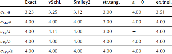
In practical cases, shimmy occurs at path frequencies below the meandering frequency, even below about half this value. This may correspond to a practical upper limit of a/λ = 0.04 or for the wavelength λ a lower limit of ca. 12.5 times the contact length (25a). It turns out that in this practical range, the agreement between the various models is good or reasonable.
5.4.2 Other Models
Two more models will be briefly discussed. These are the models of Keldysh, cf. Goncharenko et al. (1981) and Besselink (2000), and of Moreland (1954). The models are not based on the stretched string concept. They feature two degrees of freedom – the lateral deflection and the torsion deflection – and disregard the finite length of the contact zone. The single-point or straight tangent approximations of the string model have a single degree of freedom where the lateral and the angular deflections at the leading edge are linked through an algebraic relationship. The additional degree of freedom of Keldysh's and Moreland's single-point models with a nonholonomic constraint (first-order differential equation) raises the order of the description from one to two.
Keldysh's Model
This model is known to be used in the Russian aircraft industry and was published in 1945. Goncharenko employed the model for his research in shimmy of landing gears. In addition to lateral and torsional stiffnesses, damping has been included between contact patch and rim. The side force and aligning torque become expressed in terms of lateral deflection v and torsion angle β:
![]() (5.141)
(5.141)
![]() (5.142)
(5.142)
With the assumption of full adhesion, the following relation must hold regarding the direction of the path of the contact point of the rolling tire:
![]() (5.143)
(5.143)
Regarding the path curvature, a linear equation is introduced:
![]() (5.144)
(5.144)
Interesting is that Keldysh did take into account the wheel camber angle γ as an additional input variable. The transfer functions with respect to α, φ, ψ, and γ become
![]() (5.145)
(5.145)
and
![]() (5.146)
(5.146)
Surprisingly, it turns out that these transfer functions (except the one with respect to γ) correspond to the functions of Rogers (with ε = 0) (Eqns 5.102, 5.103 with ½a omitted) if, as Besselink indicated, the following equivalence conditions hold:
![]() (5.147)
(5.147)
Furthermore, comparison with the Von Schlippe approximation at steady-state shows that
![]() (5.148)
(5.148)
where, as before, CFγ designates the camber force stiffness.
Moreland's Model
This model, first published in 1954 in the paper “The story of shimmy,” used to be a popular tool in the U.S. for the analysis of aircraft shimmy. The structure is similar to that of Keldysh's model. The differences are that the damping coefficient kψ is omitted and, more important, turn slip and camber are not considered and instead of Eqn (5.144) the following relation is used:
![]() (5.149)
(5.149)
The transfer functions with respect to the slip angle that were established read
![]() (5.150)
(5.150)
![]() (5.151)
(5.151)
The fact that we are dealing here with a time constant τ gave rise to criticism and caused difficulties in attempts to fit experimental data. To make the model pure path dependent, τ should be made inversely proportional with speed V; this in addition to omitting the damping coefficient ky. It may be observed that when considering the relations (5.147), the substitution for τ
![]() (5.152)
(5.152)
leads to a transfer function with respect to α that is identical to the corresponding functions established by Keldysh and Rogers.
5.4.3 Enhanced String Model with Tread Elements
Although the string model with its simplicity and essential features served us well in gathering insight and establishing proper mathematical descriptions and useful approximations, the string model shows a behavior that in several views differs considerably from the properties of the real tire. The relaxation length σ for the tire deflection does not change with vertical load, and thus the relaxation length for the side force to yaw σFψ = σ + a does not vary sufficiently and does not approach zero when Fz → 0 as would occur with the real tire. The same discrepancy holds for the cornering stiffness. The pneumatic trail of the string model is often too large. When considering larger values of slip, that is, when sliding is allowed to occur in the contact zone, the calculated steady-state characteristics for the bare string model do not appear to be adequate as they exhibit a kink at the slip angle where the force has reached its maximum and the moment becomes equal to zero where full sliding commences. Also, when at side slip the lateral force distribution along the contact line is analyzed, it appears that a discontinuity occurs at the point of transition from adhesion to sliding. This is caused by the fact that in the range of adhesion the contact line (that is: the string) is straight and the external frictional forces are equal to the internal elastic forces and remain relatively small. From the transition point onward, the string slides over the ground and the side forces are governed by the vertical force distribution and the friction coefficient. Here the contact line gets curved to let the string tension force S contribute to the transmission of the ground forces to the tire. Finally, it can be easily assessed that the relaxation length of the bare string model does not change with increasing slip angle as is observed to occur in practice. These reasons lead to the desire to develop a model that shows a better behavior and when too complex may serve as a reference for understanding and for the development of simpler models. In the sequel, we will briefly discuss the development of the string model provided with elastic tread elements; for more information, cf. Pacejka (1966, 1981). The results concerning this model's transient and oscillatory out-of-plane behavior have already been included in the various graphs of the preceding section.
Steady-State Characteristics
Figure 5.28 depicts the structure of the model. The total deflection v is made up of the lateral deflection of the string (the carcass) vc and the lateral deflection of the tread element vp. Associated stiffnesses of carcass and tread elements are cc and cp both per unit length and the latter integrated over the tread width 2b. The string effective tension force is S, cf. Section 5.3.1. The following model constants are introduced:
![]() (5.153)
(5.153)
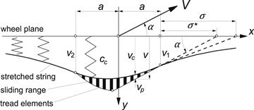
FIGURE 5.28 Enhanced string model provided with tread elements.
A parabolic vertical pressure distribution is assumed according to Eqn (3.4). At the trailing edge, a sliding range starts to build up when side slip increases. Also at the leading edge, sliding may occur when the tread element stiffness is relatively large. The bare string model does show a relatively short sliding range that grows and ultimately meets the rear sliding range at increasing side slip. We will assume that the tread element stiffness is sufficiently small to disregard front sliding.
The total deflection v at steady-state side slip in the range xt < x < a, where the tips of the elements adhere to the ground, follows the differential Eqn (5.11) with φ = 0:
![]() (5.154)
(5.154)
The deflection of the string outside the contact range is governed by the differential equation:
![]() (5.155)
(5.155)
and in the contact zone:
![]() (5.156)
(5.156)
To solve for the coordinate of the transition point xt and the five constants of integration in the solutions of Eqn (5.154) and of Eqn (5.156) for the two zones, adhesion and sliding, we need six boundary conditions. These concern zero tread element deflection at the leading edge and continuity of deflection and slope of the string and continuity of the element deflection at the transition point. The conditions read
![]() (5.157)
(5.157)
![]() (5.158)
(5.158)
![]() (5.159)
(5.159)
Once expressions for the deflection vp = v − vc and the transition point xt have been established, the force and moment can be assessed by integration along the contact length of qy over the sliding range and of cpvp over the adhesion range. The resulting formulas can be found in the original publication. We will restrict ourselves here with showing the characteristics for the values σ = 3.75a and cp/cc = 55. Figure 5.29 depicts the deflected model at a number of slip angles. In Figure 5.30, the force and moment characteristics have been presented with along the abscissa the quantity θcα. The composite model parameter θc is defined as
![]() (5.160)
(5.160)
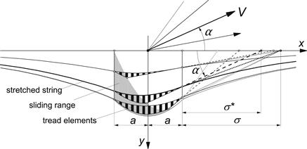
FIGURE 5.29 The enhanced string tire model at increasing slip angles showing growing sliding range and decreasing ‘intersection’ length σ∗.
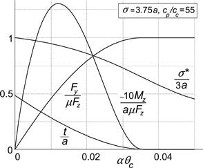
FIGURE 5.30 Steady-state side-slip characteristics of the string model with tread elements.
For transient tire analysis, the relaxation length for the leading edge, σ for the bare string model and σ∗ for the model with tread elements here defined as the distance between leading edge and the point of intersection of wheel plane and elongation of the straight contact line (Figures 5.8, 5.28, and 5.29), is of importance. We have
![]() (5.161)
(5.161)
The variation of this ‘intersection length’ σ∗ with slip angle has been plotted as well. The parameters have been chosen such that at α = 0, we have σ∗ = 3a.
The diagram also contains the curve for the pneumatic trail t = −Mz/Fy. At α = 0, the value of the pneumatic trail becomes t = 0.49a which is much more in accordance with experimental findings than what we had with the bare string model. The value 0.49a also supports the magnitude that had been found for the relaxation length for the force to side slip σFα = σ∗ + a − t = 3.51a as indicated in Table 5.1, cf. Eqn (5.72).
Expressions for the slip stiffnesses, the pneumatic trail and the relaxation length, and their relationship with vertical load will be presented in the subsequent subsection, where the linear model is discussed.
Non-Steady-State Behavior at Vanishing Sliding Range (Linear Analysis)
We will restrict ourselves to the derivation of the response to the slip angle α and use conversion formula (5.39), with σ replaced by σ∗ (5.171) to obtain the response functions to turn slip φ and (5.36, 5.37) for the responses to y and ψ. For the total deflection v, or transformed V, Eqns (5.11, 5.14) and thus (5.16) hold in general. With A representing the transformed α, we get
![]() (5.162)
(5.162)
With the Laplace transformed version of Eqn (5.156), the differential equation for Vc is obtained:
![]() (5.163)
(5.163)
with solution:
![]() (5.164)
(5.164)
The three integration constants can be determined by using the boundary conditions at the leading and trailing edges (5.157, 5.159):
![]() (5.165)
(5.165)
![]() (5.166)
(5.166)
with
![]() (5.167)
(5.167)
![]() (5.168)
(5.168)
Integration of Vp = V − Vc times the stiffness cp over the contact length yields the transformed expressions for the force Fy and, after multiplication with x, the moment ![]() . The following formulas are obtained for their transfer functions to the slip angle α:
. The following formulas are obtained for their transfer functions to the slip angle α:
![]() (5.169)
(5.169)
 (5.170)
By letting p → 0 in the expressions for σ∗ = V1/A (cf. (5.162), x = a) and the transfer functions (5.169, 5.170), the relaxation length and the slip stiffnesses may be assessed. We find
![]() (5.171)
(5.171)
![]() (5.172)
(5.172)
![]() (5.173)
(5.173)
![]() (5.174)
(5.174)
and the pneumatic trail:
![]() (5.175)
(5.175)
It is of interest to examine how these quantities vary with vertical load Fz. For this purpose, we assume that the contact length varies with the square root of the radial tire compression and that the load is a linear function of the compression. Then we find that, if at the nominal or static load Fz0 half the contact length is denoted by ao, the Fz vs α relationship is described by
![]() (5.176)
(5.176)
This, introduced in the above expressions, yields the characteristics shown in the diagram of Figure 5.31. The various nondimensional quantities have been presented both for the bare string model and for the enhanced model. As has been expected, we now see that the relaxation length for the force and moment responses to yaw, σ∗ + a, vanishes when the load tends to zero. The pneumatic trail's ratio to half the contact length is a lot more realistic when the tread elements are added. The same holds for the cornering and aligning stiffnesses shown in Figure 5.32. With the enhanced model, the curves both start at the origin and exhibit a realistic shape. The feature, usually exhibited by passenger car tires, that the cornering stiffness bends downwards after it has reached the peak (cf. Figure 1.3) may be attributed to the reduced lateral stiffness of the tire cross section at higher vertical compression, cf. Pacejka (1981, p. 729 or 1971, p. 698) for an analytical formula.
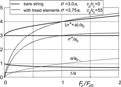
FIGURE 5.31 The variation of the relaxation length and half the contact length as a ratio to the static value of the latter and the ratio of the pneumatic trail to half the contact length with normalized vertical load both for the bare string model and for the model with tread elements.
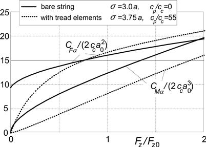
FIGURE 5.32 The variation of nondimensionalized cornering and aligning stiffnesses with normalized vertical load both for the bare string model and the model with tread elements.
The frequency response functions for the enhanced model are presented in Figures 5.33 and 5.34. They may be compared with the plots of Figures 5.14 and 5.15 which hold for the bare string model. The model parameters are again: σ = 3.75a, cp/cc = 55. An important result of the analysis is that expressions (5.70, 5.72, 5.74, 5.79– 5.81) for relaxation lengths and cutoff frequencies are the same for the bare string model and the enhanced model if, in these expressions, σ is replaced by σ∗ defined by (5.171).
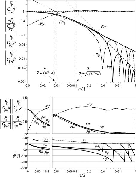
FIGURE 5.33 Frequency response functions of the string model with tread elements for the side force with respect to various motion input variables. For the response to α, a first-order approximation with the same cutoff frequency, ωs = 1/(σ∗ + a), has been added (Fα1). Three ways of presentation have been used: log–log, lin–log, and lin–lin. The model parameters are: σ = 3.75a, cp/cc = 55 which leads to σ∗ = 3a, t = 0.49a.
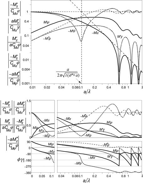
FIGURE 5.34 Frequency response functions of string model with tread elements for the aligning torque with respect to various motion input variables. Same conditions as in Figure 5.33. The response functions of the moment due to tread width ![]() have been added.
have been added.
For comparison, the plots for the step responses and for the frequency response functions have been presented in Figures 5.21–5.27 together with results of other models. Also, Table 5.1 (p. 256) contains data computed with the new model. The general course of the curves is similar. Important differences with respect to the bare string model are the considerable shift of the cutoff frequency of the ![]() response to α and similarly of Fy to φ and, together with these, the meandering frequency where the dip of the
response to α and similarly of Fy to φ and, together with these, the meandering frequency where the dip of the ![]() response to ψ occurs. The reduction of the pneumatic trail t is responsible for the increase of the cutoff frequency.
response to ψ occurs. The reduction of the pneumatic trail t is responsible for the increase of the cutoff frequency.
Experimental results assessed on a 2.5-m diameter steel drum have been presented in Figure 5.35. The responses are depicted in the Nyquist diagram (cf. Figures 5.17 and 5.18) as a ratio to their values assessed at steady-state side slip. Two light truck tires have been tested at a vertical load of Fz = 10 kN. Both tires possess the same cross-ply construction but exhibit a different tread design. The original tire shows a block tread design (central rib with transverse blocks, oval foot print), which is relatively weak in the longitudinal direction at the sides of the contact patch. The modified tire is provided with circumferential ribs (three ribs, almost rectangular foot print) making the tread relatively stiff in the longitudinal direction. As expected, the ribbed tire generates more resistance against turning which is reflected by a larger moment due to tread width ![]() and consequently a considerably smaller phase lag of the resulting self-aligning torque −Mz. The side force does not appear to be much affected at least in the larger wavelength range.
and consequently a considerably smaller phase lag of the resulting self-aligning torque −Mz. The side force does not appear to be much affected at least in the larger wavelength range.
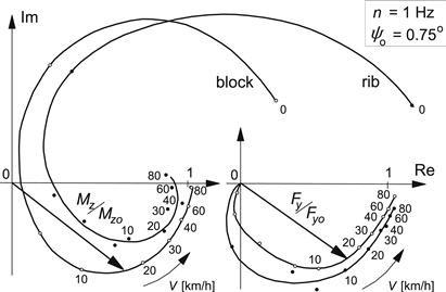
FIGURE 5.35 Frequency response plots of Fy and Mz to ψ for two light truck tires with same bias-ply carcass but different tread patterns. Measurements were performed on a 2.5-m drum at a vertical load of 10 kN, a yaw amplitude of 0.75° at a frequency n = 1 Hz.
In Table 5.2, parameters estimated from the measurements have been listed. The intersection length or deflection relaxation length σ∗ was determined from the formula:
![]() (5.177)
(5.177)
TABLE 5.2 Parameters for Two 9.00–16 Tires with Different Tread Patterns
| Blocks | Ribs | |
| ro | 0.5 m | 0.5 m |
| a | 0.115 m | 0.08 m |
| b | 0.092 m | 0.10 m |
| t | 0.53a | 0.82a |
| σ∗ | 2.4a | 2.8a |
| Fz | 10 kN | 10 kN |
| CFα | 64 kN/rad | 53 kN/rad |
| CMα | 3.9 kNm/rad | 3.5 kNm/rad |
| CFy | 165 kN/m | 175 kN/m |
| κ∗ | 0.25 CMαa | 1.0 CMαa |
When considering the relation a/λ = an/V with Vkm/h = 3.6 Vm/s, the value for the nondimensional path frequency at V = 10 km/h and an excitation frequency of 1 Hz becomes a/λ = 0.0414 which roughly corresponds with that indicated on the thin tire model curve of Figure 5.18.
5.5 Tire Inertia Effects
It has been found experimentally that higher frequencies and greater speeds of travel bring about an increasingly important deviation of the response with respect to the kinematic representation with dynamic influences disregarded.
Figure 5.36 presents an example of response curves obtained experimentally. The response curves for the moment Mz and the side force Fy to the yaw angle ψ have been shown as a function of the speed of travel V for fixed values of the excitation frequency n of the imposed yaw oscillation. The force and moment outputs are given as a ratio to their steady-state values (at ωs = ω = 0) indicated by the subscript 0.
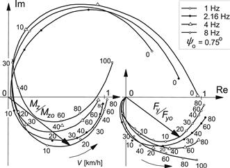
FIGURE 5.36 Frequency response plots of Fy and Mz to ψ for light truck tire with block tread pattern. Measurements were performed on a 2.5-m drum at a vertical load of 10 kN, a yaw amplitude of 0.75° and at four different time frequencies.
We observe that for higher frequencies the curves of the moment response appear to shift upward. The force response curves, on the other hand, show an increase in amplitude while the phase lag remains approximately unchanged for constant wavelength λ = V/n.
5.5.1 First Approximation of Dynamic Influence (Gyroscopic Couple)
In the low frequency range, n < 10 Hz, the aligning torque appears to be affected most by the inertia of the tire. A simple addition to the kinematic model may approximately describe the dynamic changes in the response of the moment. In this theory, the gyroscopic couple due to the lateral deformation rate of the lower portion of the tire has been introduced as the only dynamic influence. It is assumed here that the dynamic forces have a negligible effect on the distortion of the tire.
The gyroscopic couple about the vertical axis is proportional to the wheel rotational speed and the time rate of change of the tilt (camber) distortion of the tire, cf. Figure 5.37. Since this distortion is connected with the lateral deflection of the lower part of the tire and the side force Fy is proportional to this deflection, we have, for the gyroscopic couple,
![]() (5.178)
(5.178)
in which t denotes the time. The tire constant Cgyr is proportional to the tire mass mt and inversely proportional to the lateral stiffness CFy of the standing tire. We have, with the nondimensional quantity cgyr introduced,
![]() (5.179)
(5.179)
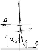
FIGURE 5.37 The average tilt angle of the peripheral line of the deflected tire.
The total moment which acts upon the wheel is now composed of the moment due to lateral tire deformation ![]() and that due to longitudinal anti-symmetric tread deformations
and that due to longitudinal anti-symmetric tread deformations ![]() and finally the gyroscopic couple Mz,gyr:
and finally the gyroscopic couple Mz,gyr:
![]() (5.180)
(5.180)
With this simple addition to the enhanced stretched string tire model (provided with tread elements distributed over the assumedly rectangular contact area), calculations have been performed. Figure 5.38 shows the Nyquist plot of the responses along with the curves ωs a = 2π na/V = 2π a/λ. It should be noted that the vector of the gyroscopic couple is directed perpendicularly to the vector of the lateral force. For the range of frequencies considered, the simple approximate dynamic extension theory gives a good representation of the effect on the moment response curves. However, the theory does not account for the dynamic changes in the force response.
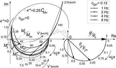
FIGURE 5.38 The influence of the frequency of the yaw oscillation on the dynamic response according to the simple approximate model extension using the gyroscopic couple due to the lateral tire deflection time rate of change.
5.5.2 Second Approximation of Dynamic Influence (First Harmonic)
More complex theories as developed by Pacejka (1973a) and by Strackerjan (1976) and more recently by Maurice (2000), cf. Chapter 9, yield better results also with respect to the force response and extends to higher frequencies covering the first natural frequencies of the out-of-plane tire dynamic behavior. In these theories, the tire circular belt is considered to move not only about a longitudinal axis but also about a vertical axis and in the lateral direction. The belt rotation about the vertical axis gives rise to a gyroscopic couple about the longitudinal axis which on its turn results in a change in slip angle which influences Fy (and also Mz).
The interesting feature of the approach followed in the first reference mentioned above is that the kinematic theory and response equations as treated in Sections 5.3 and 5.4 with tire inertia equal to zero can be employed. The kinematic part of the model will be considered to be subjected to a different, effective, set of input motion variables. Instead of taking the motion of the actual wheel plane defined by ![]() and ψ (or α and φ), an effective input is introduced that is defined as the lateral and the yaw motion of the line of intersection of the ‘dynamic’ belt plane and the road surface
and ψ (or α and φ), an effective input is introduced that is defined as the lateral and the yaw motion of the line of intersection of the ‘dynamic’ belt plane and the road surface ![]() . Figure 5.39 depicts the situation. The dynamic belt plane is defined as the virtual center plane of the belt of the tire that is displaced with respect to the rim through the action of lateral inertial forces only. These inertial forces distributed along the circumference of the belt are approximated in such a way that only the forces resulting from the zeroth and first modes of vibration are taken into account, that is: as if the belt would remain circular. Harmonics of second and higher order are neglected in the dynamic part of the model. We have, for the approximate dynamic lateral, camber, and yaw deflections, respectively,
. Figure 5.39 depicts the situation. The dynamic belt plane is defined as the virtual center plane of the belt of the tire that is displaced with respect to the rim through the action of lateral inertial forces only. These inertial forces distributed along the circumference of the belt are approximated in such a way that only the forces resulting from the zeroth and first modes of vibration are taken into account, that is: as if the belt would remain circular. Harmonics of second and higher order are neglected in the dynamic part of the model. We have, for the approximate dynamic lateral, camber, and yaw deflections, respectively,
 (5.181)
with the total tire deflections composed of dynamic and static parts (the latter resulting from external ground forces):
 (5.182)
and stiffnesses of the whole belt with respect to the rim Cy, Cγ, and Cψ. Furthermore, the equations contain effective tire inertia parameters mt, It, and polar moment of inertia Itp. The effective inputs to the kinematic model are defined by
 (5.183)
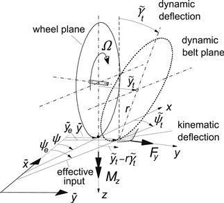
FIGURE 5.39 ‘Dynamic’ average plane deflection of belt and associated effective input.
With the aid of these equations plus the kinematic tire equations (e.g. Von Schlippe's approximate Eqns (5.87, 5.88, 5.92, 5.93) with (5.36, 5.37) and (5.32) for ![]() with inputs
with inputs ![]() replaced by effective inputs
replaced by effective inputs ![]() , the frequency response functions of the ground force Fy and moment
, the frequency response functions of the ground force Fy and moment ![]() with respect to the actual inputs
with respect to the actual inputs ![]() may be readily established.
may be readily established.
For applications in vibratory problems associated with wheel suspension and steering systems, it is of greater interest to know the response of the equivalent force and moment that would act on the assumedly rigid wheel with tire inertia included at the contact center. The equivalent force and moment are obtained as follows:
![]() (5.184)
(5.184)
This result should correspond to the force and moment measured in the wheel hub, Fy,hub and Mz,hub, after these have been corrected for the inertial force and moment acting on the assumedly rigid wheel plus tire (inertia between load cells and ground surface). With inertia parameters of wheel plus tire, we find, for this correction,
![]() (5.185)
(5.185)
When lifted from the ground, the equivalent ground to tire forces vanish if the frequency of excitation is not too high (low with respect to the first natural frequency of the tire).
For the set of parameter values measured on a radial-ply steel-belted tire listed in Table 5.3, the amplitude and phase of the equivalent moment as a response to yaw angle have been computed and are presented in Figure 5.40 as a function of the excitation frequency ![]() . Experimentally obtained curves up to a maximum of 8 Hz (on 2.5 m drum) have been added. The phase lag that occurs in the lower frequency range is largely responsible for the creation of self-excited wheel shimmy. The influence of tire inertia is evident: the phase lag changes into phase lead at higher values of speed (similar as in Figure 5.38). In contrast to the dynamic response depicted in Figure 5.41, the kinematic model response (without the inclusion of tire inertia) would produce the same response at equal wavelengths, λ = V/n, irrespective of the value of the speed of travel V.
. Experimentally obtained curves up to a maximum of 8 Hz (on 2.5 m drum) have been added. The phase lag that occurs in the lower frequency range is largely responsible for the creation of self-excited wheel shimmy. The influence of tire inertia is evident: the phase lag changes into phase lead at higher values of speed (similar as in Figure 5.38). In contrast to the dynamic response depicted in Figure 5.41, the kinematic model response (without the inclusion of tire inertia) would produce the same response at equal wavelengths, λ = V/n, irrespective of the value of the speed of travel V.
TABLE 5.3 Parameters for Car Tire Model with Dynamic Belt Extension (2nd Approximation)
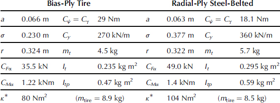
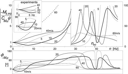
FIGURE 5.40 Amplitude and phase response of equivalent aligning torque (as if acting from ground on rigid wheel tire) to yaw angle as a function of time frequency of excitation [Hz] computed using Von Schlippe approximation and exact ![]() extended with dynamic theory according to second approximation with dynamic belt. Model parameters are listed in Table 5.3 (radial steel belted tire). Curves hold for given speed of travel V [m/s]. Experimental results are given up to a frequency of 8 Hz. The yaw natural frequency of the free non-rotating tire with fixed wheel spindle is n00.
extended with dynamic theory according to second approximation with dynamic belt. Model parameters are listed in Table 5.3 (radial steel belted tire). Curves hold for given speed of travel V [m/s]. Experimental results are given up to a frequency of 8 Hz. The yaw natural frequency of the free non-rotating tire with fixed wheel spindle is n00.
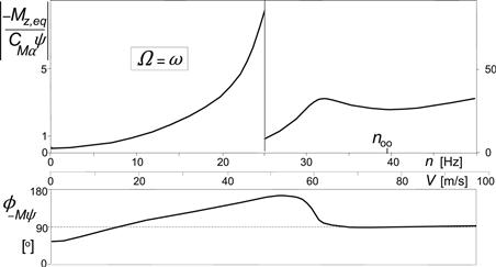
FIGURE 5.41 Amplitude and phase response as a function of frequency with the frequency of excitation equal to that of wheel revolution.
The resonance frequencies, which at speeds close to zero approach a value somewhat larger than the natural frequency of the free non-rotating tire, n00, appear to separate at increasing speed. Vibration experiments performed on a free tire (not contacting the road) for the purpose of obtaining the values of certain tire parameters gave a clear indication that a reduction of the lowest resonance frequency arises when the wheel is rotated around the wheel spin axis at higher speeds of revolution.
Nyquist plots for the Mz,eq and Fy,eq responses to ψ have been presented in Figures 5.42 and 5.43. Both for the bias-ply and for the radial steel-belted tire of Figure 5.40, theoretical and experimental results are shown. Parameters are according to Table 5.3. For each of the curves, the excitation frequency remains constant while the speed varies along the curve.
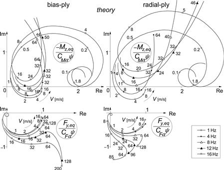
FIGURE 5.42 Theoretical frequency response Nyquist plots of side force and aligning torque to yaw angle for different time frequencies. Same conditions as in Figure 5.40.
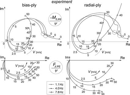
FIGURE 5.43 Experimental frequency response Nyquist plots of side force and aligning torque to yaw oscillations for a radial and a bias-ply car tire measured on a 2.5-m drum.
An increase in frequency tends to raise the moment curves while the force response curves appear to expand with the phase angle at a given wavelength remaining not much changed. The typical differences between the two types of tires, notably in the shape of the upward ends of the moment curves where the speed assumes high values, are well represented in the theoretical diagrams.
We may conclude that the simple first approximation appears to give a considerable improvement for the moment response in the lower frequency range, while for the force response and the higher frequency excitations the inclusion of the dynamics of the belt up to the first modes of vibration is required.
Since we have here a dynamic model extension that allows the use of existing kinematic (mass less) models, we have been able to investigate the effect of tire inertia on these models. However, for the sake of simplicity these models have been restricted to a linear description allowing straightforward frequency response analysis. Extension into the nonlinear regime in the time domain is cumbersome for models including a finite contact length (retardation) effect (although an approximate nonlinear Von Schlippe model may be established by attaching nonlinear springs to the wheel plane at the leading and trailing edges the tips of which follow the path as if we had full adhesion) and also because in the dynamic extension, Eqns (5.181–5.183), the function Fy = Fy(α′) would be needed in an inverse form.
To further develop mathematical models that can be used under conditions that include short wavelengths, higher frequencies, and large (combined) slip, a different route appears to be more promising. The adopted principle is: separate modeling of the flexible belt with carcass and the contact patch with its transient slip properties. The theory of the non-steady-state rolling and slipping properties of the brush model helps in this modeling effort. In Chapter 9, this advanced model will be discussed.
For less demanding cases (large wavelength, low frequency), the straight tangent or single-point contact models may be employed. Such models may be used in combination with the approximate dynamic extension that accounts for the gyroscopic couple due to the lateral deflection velocity. Furthermore, these simple models can be easily adapted to cover large slip nonlinear behavior, cf. Eqns (5.125, 5.126, 5.128) or (5.130–5.132) and Eqn (5.178) with Fy replaced by CFyv0. Chapter 7 is devoted to the treatment of the very useful and relatively simple, possibly nonlinear, single contact point transient slip models. With that single-point contact model, the problem of cornering (and braking) on undulated road surfaces can be made more accessible for vehicle simulation studies. First, we will address this difficult subject in the subsequent section using exact string models with and without tread elements which shows the deeper cause of the associated loss in cornering power.
5.6 Side Force Response to Time-Varying Load
In studies by Metcalf (1963), Pacejka (1971), and more recently by Laermann (1986) and by Takahashi (1987) and Pacejka (1992), it was found that the average value of the side force generated by a constant slip angle is reduced as a result of a periodical change of the vertical load. This reduction may be considerable and appears to depend on the amplitude of the vertical load variation as a ratio to the static load, on the wavelength of the motion, the speed of travel, and on the magnitude of the slip angle. In Chapter 7, a more practical approach based on the single contact point model (that means: for accuracy limited to relatively large wavelengths) is adopted to model the non-steady-state behavior at varying vertical load, including high levels of slip. To lay the basis for that theory, we will employ the advanced string model with tread elements that was developed in Section 5.4.3 for the case of a constant vertical load. The presence of tread elements turns out to be crucial to properly model the loss of side force when cornering on an undulated road surface. As in Section 5.4.3, only small slip angles will be considered allowing the theory to remain linear. First, we will develop the model based on the advanced string model with tread elements. Then, to simplify the model description, an adapted bare string model will be introduced and used in the further calculations.
5.6.1 String Model with Tread Elements Subjected to Load Variations
Figure 5.44 shows the tire model in two successive positions while the wheel moves at a constant (small) slip angle over an undulated road surface which causes the contact length to vary with distance traveled s. When the contact center C is moved a distance Δs, the following changes occur simultaneously: lateral shift of the wheel plane, forward rolling, and change in contact length. These changes influence the position of the leading and trailing edges of the string. The ![]() coordinates of these points are:
coordinates of these points are:
![]() (5.186)
(5.186)
the changes of which become
![]() (5.187)
(5.187)
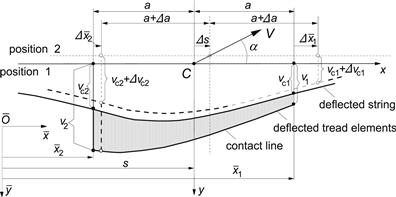
FIGURE 5.44 Two successive positions of tire model with varying contact length at constant slip angle α (sliding not considered).
The changes in front and rear lateral string deflections vc1,2 are composed of various contributions. For the increment of the deflection at the leading edge Δvc1 we obtain
1. due to lateral wheel displacement ![]() :
:
![]() (5.188a)
(5.188a)
2. due to loss of contact at the trailing edge ![]() :
:
![]() (5.188b)
(5.188b)
3. due to loss of contact at the leading edge ![]() :
:
![]() (5.188c)
(5.188c)
4. due to longitudinal displacement of leading edge ![]() :
:
![]() (5.188d)
(5.188d)
Similar expressions are obtained for the contributions to the change of the lateral deflection at the rear ![]() . The contact length-dependent coefficients appearing in the equations are
. The contact length-dependent coefficients appearing in the equations are
![]() (5.189)
(5.189)
![]() (5.190)
(5.190)
![]() (5.191)
(5.191)
![]() (5.192)
(5.192)
They are derived from solutions of the differential equations for the shape of the string deflection (Eqns (5.155, 5.156)). For the parameters employed, we refer to Eqn (5.153). From the increments (5.187, 5.188), the following differential equations are established for the unknown string deflections vc1 and vc2:
![]() (5.193)
(5.193)
![]() (5.194)
(5.194)
The two remaining unknowns v1 and v2 representing the total lateral deflections and consequently the distances between wheel plane and contact line at the leading and trailing edges are found by considering the following. In the rolling process of a side slipping tire with a continuously changing contact length, in general, three intervals can be distinguished during the interval of the loading cycle where contact with the road exists. In Figure 5.45, the load variation together with the corresponding variation of the contact length 2a of a side slipping tire that periodically jumps from the road has been shown in the road plane ![]() for the interval that contact exists. Immediately after the first point touches the road, the contact line grows in two directions (interval I). This growth continues until the second interval II is reached, where growth of contact takes place only at the front, and at the rear loss of contact occurs. Finally, in the third interval III, loss of contact at both ends takes place until the tire leaves the road. When the tire does not leave the road, an additional interval II occurs before interval I is reached again and the cycle starts anew. In less severe cases, intervals I and III may not occur. We then have the relatively simple situation of continuous growth of contact at the front and loss of contact at the rear.
for the interval that contact exists. Immediately after the first point touches the road, the contact line grows in two directions (interval I). This growth continues until the second interval II is reached, where growth of contact takes place only at the front, and at the rear loss of contact occurs. Finally, in the third interval III, loss of contact at both ends takes place until the tire leaves the road. When the tire does not leave the road, an additional interval II occurs before interval I is reached again and the cycle starts anew. In less severe cases, intervals I and III may not occur. We then have the relatively simple situation of continuous growth of contact at the front and loss of contact at the rear.
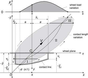
FIGURE 5.45 On the development of the contact line of the tire model with tread elements that periodically loses contact with the road.
The unknowns v1 and v2 and the coordinate of the contact points in the ![]() plane are obtained as follows (cf. Figure 5.45):
plane are obtained as follows (cf. Figure 5.45):
![]() (5.195a)
(5.195a)
![]() (5.195b)
(5.195b)
![]() (5.195c)
(5.195c)
By means of numerical integration, Eqns (5.193, 5.194) have been solved with the aid of the Eqns (5.195) and the expressions (5.189–5.192) for the case formulated below in which the vertical tire deflection ρ has been given a periodic variation with amplitude ![]() greater than the static deflection ρo, so that periodic loss of contact between tire and road occurs.
greater than the static deflection ρo, so that periodic loss of contact between tire and road occurs.
The static situation will be indicated with subscript o. The tire radius is denoted with r. The vertical deflection and the contact length are governed by the equations
![]() (5.196)
(5.196)
![]() (5.197)
(5.197)
The numerical values of the parameters of the system under consideration are
![]()
![]() (5.198)
(5.198)
In Figure 5.46, the calculated variation of contact length 2a (oval curve), the path of the contact points (lower curve AB), and the course of the points of the string at the leading and trailing edge (AC and BC) have been indicated. Two positions of the tire have been depicted, one in interval II and the other in interval III.
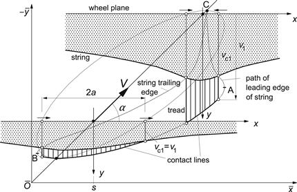
FIGURE 5.46 The deflected tire model in two positions during the interval of contact with the road.
It is necessary that the calculations in the numerical integration process be carried out with great accuracy. A small error gives rise to a rapid build up of deviations from the correct course. In the case considered above, the integration time is limited and accurate results can be obtained. In cases, however, where continuous contact between tire and road exists, a long integration time is needed before a steady-state situation is attained, which is due to the fact that the exact initial conditions of a periodic loading cycle are not known. For this sort of situation, the exact method described above is difficult to apply due to strong drift of vc2 in particular.
For further investigation of the effect of a time-varying load, we will turn to an approximate method based on the string model without tread elements.
5.6.2 Adapted Bare String Model
The use of this model is much simpler since the deflections at both edges are independent of each other. Drift does not occur in the calculation process. In Figure 5.47, the deflected model has been shown in interval II. For the three intervals, the following sets of equations apply:
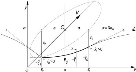
FIGURE 5.47 On the development of the contact line of the bare string model.
growth of contact at leading edge:
![]() (5.199a)
(5.199a)
![]() (5.199b)
(5.199b)
![]() (5.199c)
(5.199c)
![]() (5.199d)
(5.199d)
growth of contact at trailing edge:
![]() (5.200a)
(5.200a)
![]() (5.200b)
(5.200b)
![]() (5.200c)
(5.200c)
![]() (5.200d)
(5.200d)
loss of contact at leading edge:
![]() (5.201a)
(5.201a)
![]() (5.201b)
(5.201b)
![]() (5.201c)
(5.201c)
loss of contact at trailing edge:
![]() (5.202a)
(5.202a)
![]() (5.202b)
(5.202b)
![]() (5.202c)
(5.202c)
Solutions of the above equations show considerable differences from the results obtained using the more advanced model with tread elements. The most important difference is the fact that with the simple model the lateral force does not gradually drop to zero as the tire leaves the ground.
In order to get better agreement, we will introduce a nonconstant relaxation length σ = σ∗(a) that is a function of the contact length 2a and thus of the vertical load. We take σ∗ equal to the relaxation length of the more advanced model according to Eqn (5.171).
Figure 5.48 presents the variation of relaxation length and contact length as a function of the vertical load as calculated for the current parameter values (5.198).
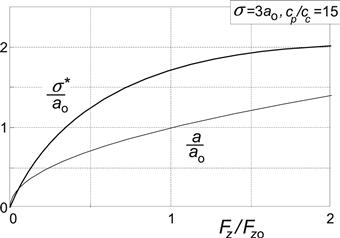
FIGURE 5.48 The calculated variation of half the contact length and the relaxation length as a ratio to the static half contact length versus the vertical load ratio for the model with tread elements using Eqn (5.171).
In Figure 5.49, a comparison is made between the results of the three models: without tread elements, with tread elements (exact), and according to the approximation with varying σ = σ∗(a). The calculations have been carried out for the parameter values (5.198). The approximate path of contact points shows good agreement with the path for the exact model with tread elements. When the tread elements are omitted, we have the bare string model for which the path becomes wider and the lateral deflections greater.
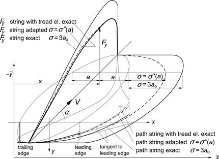
FIGURE 5.49 Paths of contact points and variations of the side force according to three models.
5.6.3 The Force and Moment Response
The lateral force Fy and the moment Mz which act on the tire can be assessed with good approximation through the following simplified formulas. In their derivations, we have replaced the contact line by the straight line connecting the beginning and end points of the contact line (Von Schlippe's approach). For the model with tread rubber elements, we obtain
![]() (5.203)
(5.203)
![]() (5.204)
(5.204)
and, for the model without tread elements,
![]() (5.205)
(5.205)
![]() (5.206)
(5.206)
In these expressions, the following quantities have been introduced:
![]() (5.207)
(5.207)
and
![]() (5.208)
(5.208)
in which A, B, and B∗ are given by expressions (5.189–5.192).
For the sake of completeness, the formulas for the moment have been added. However, we will restrict ourselves to the discussion of the variation of the force. For the three models considered, the variation of the cornering force has been shown in the same Figure 5.49. As expected, the approximate and exact theories drop to zero at the point of lift-off, whereas the force acting on the simple string model remains finite, at least under the here assumed condition of no sliding. The correspondence between exact and approximate solutions of the path and of the side force is satisfactory, and we will henceforth use the approximate method according to the adapted bare string model for the investigation of the model with tread elements.
For a series of deflection amplitudes ![]() and wavelengths λ, the variation of the cornering force, or rather of the cornering stiffness, has been calculated. Since during loss of contact the vertical load remains zero, the period of the total loading cycle must become longer in order to keep the average vertical load unchanged. This change in period has been taken into account in the calculation of the average side force or cornering stiffness CFα.
and wavelengths λ, the variation of the cornering force, or rather of the cornering stiffness, has been calculated. Since during loss of contact the vertical load remains zero, the period of the total loading cycle must become longer in order to keep the average vertical load unchanged. This change in period has been taken into account in the calculation of the average side force or cornering stiffness CFα.
Figures 5.50 and 5.51 show the final result of this investigation, viz. the cornering stiffness averaged over one complete loading cycle as a function of the vertical deflection amplitude ![]() and the path wavelength λ for both models with and without tread elements, that is: with the adapted bare string model and with the original bare string model. With the parameter values σ = 3ao and cp = 15cc, the relaxation length of the more advanced model with tread elements at the static load becomes
and the path wavelength λ for both models with and without tread elements, that is: with the adapted bare string model and with the original bare string model. With the parameter values σ = 3ao and cp = 15cc, the relaxation length of the more advanced model with tread elements at the static load becomes ![]() . For the model without tread rubber, the relaxation length has been taken equal to σ = 2ao.
. For the model without tread rubber, the relaxation length has been taken equal to σ = 2ao.
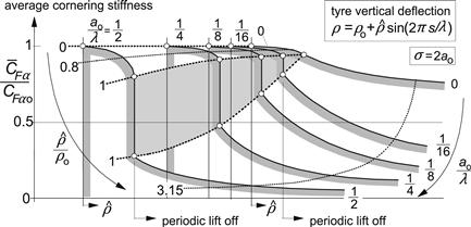
FIGURE 5.50 Computed variation of average cornering stiffness with amplitude of the vertical tire deflection, ρ, and path frequency, 1/λ, for the bare string model.
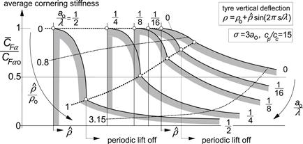
FIGURE 5.51 Computed variation of average cornering stiffness with amplitude of the vertical tire deflection (ρ) and path frequency (1/λ) using the adapted bare string model that approximates the string model with tread elements.
The figures clearly illustrate the unfavorable effect of increasing the amplitude ![]() and the path frequency (decreasing the wavelength λ). The curve at zero path frequency is purely due to the nonlinear variation of the cornering stiffness CFα versus vertical load Fz shown in Figure 5.32 (cf. Figure 1.3 and discussion on the effect of load transfer in Chapter 1, Figure 1.7) and reflects the ‘static’ drop in average cornering stiffness. A pronounced difference between the response of both types of models is the sudden drop in average cornering stiffness that shows up in the curves of the bare string model when the frequency is larger than zero and the deflection amplitude reaches the value of the static deflection. This is in contrast to the gradual variation in average cornering stiffness which is observed to occur with the more advanced model, and no doubt also with the real tire. Furthermore, the more advanced model with tread elements already shows a noticeable decrease in average cornering stiffness before the tire starts to periodically leave the ground. The ‘dynamic’ drop is represented by the dotted curves along which the path frequency changes and the deflection amplitude remains the same. The very low level, to which the average stiffness is reduced, once loss of contact occurs, is of the same order of magnitude for both tire models.
and the path frequency (decreasing the wavelength λ). The curve at zero path frequency is purely due to the nonlinear variation of the cornering stiffness CFα versus vertical load Fz shown in Figure 5.32 (cf. Figure 1.3 and discussion on the effect of load transfer in Chapter 1, Figure 1.7) and reflects the ‘static’ drop in average cornering stiffness. A pronounced difference between the response of both types of models is the sudden drop in average cornering stiffness that shows up in the curves of the bare string model when the frequency is larger than zero and the deflection amplitude reaches the value of the static deflection. This is in contrast to the gradual variation in average cornering stiffness which is observed to occur with the more advanced model, and no doubt also with the real tire. Furthermore, the more advanced model with tread elements already shows a noticeable decrease in average cornering stiffness before the tire starts to periodically leave the ground. The ‘dynamic’ drop is represented by the dotted curves along which the path frequency changes and the deflection amplitude remains the same. The very low level, to which the average stiffness is reduced, once loss of contact occurs, is of the same order of magnitude for both tire models.