The single track vehicle is more difficult to study than the double track automobile and poses a challenge to the vehicle dynamicist. Stability of motion is an important issue and it turns out that the stabilizing actions of the human rider are essential to properly handle the vehicle. Steady-state cornering behavior can be analyzed in a straightforward manner together with the examination of the stability of the equilibrium motion. While for an automobile only the lateral and yaw degrees of freedom are minimally needed to perform such an analysis, a single track vehicle requires in addition the inclusion of the roll degree of freedom for the steady-state cornering study and the steer angle as a free motion variable to examine the stability. For better correspondence with reality also the torsion of the front frame with respect to the mainframe about an axis perpendicular to the steering axis is of importance. When the non-linear problem at higher cornering accelerations is investigated, a major difficulty is formed by the fact that the separation of lateral and vertical motions is not possible since due to the roll angle of the motorcycle a strong interaction between in-plane and lateral motions occurs. This is in contrast to the situation of a double track vehicle where the roll angle remains relatively small.

Performance of the vehicle in terms of handling properties is a matter that can be studied theoretically only if a proper model of the stabilization capabilities of the human rider is available. While in an automobile the driver normally uses the steering wheel to control the vehicle direction of motion, the pilot of a motorcycle has two or three quantities to his disposal to steer and stabilize the vehicle. These are: the steer angle or the steer torque and the lean angle (and possibly the lateral shift) of the upper torso.

In the past, a number of researchers studied the performance of the single track vehicle. Noteworthy is the very early theoretical study of Whipple (1899) on the stability of the motion of the bicycle with the tires assumed to be rigid. Sharp (1971) was one of the first to investigate the motorcycle’s stability using a proper tire model. Later, the torsional compliance of the frame was introduced (Sharp and Alstead 1980a and Spierings 1981), which appeared to have a marked effect on the stability of the wobble mode (steering oscillations). In 1980 and 1983 Koenen reported an elaborate study on the stability also at large lateral curving accelerations which involve large roll angles and interaction of in-plane and lateral dynamics of the complex system. As the model representing the vehicle becomes more complex and impacts from road obstacles become more demanding to model the tire, e.g. the kick-back phenomenon, multi-body vehicle models and advanced dynamic tire models become indispensable for proper and efficient research. We refer to the following publications: Iffelsberger (1991), Wisselman et al. (1993), Breuer et al. (1998), Sharp et al. (2001a) and Berritta et al. (2000). Significant experimental results relating to the influence of design parameters on the damping of the main oscillatory modes have been given by Bayer (1988), Takahashi et al. (1984) (tire parameters), Hasegawa (1985) and Nishimi et al. (1985). In 1978, 1985, and 2001 Sharp published extensive reviews of the state of the art existing. An extensive more recent interesting review paper on the dynamics of motorcycles and bicycles has been published by Limebeer and Sharp (2006).

Important literature is available on rider behavior both as an active controller and stabilizer and as a passive part of the structure. We refer to the publications: Weir (1972), Nishimi et al. (1985), Katayama et al. (1988,1997), Cossalter et al. (1999), Biral et al. (2001) and Sharp (2010). The first one studies stabilizing feedback control, the second reference deals with passive rider model behavior, the third couple of papers discuss, among other things, maneuvering effort while the latter three papers address the problem of optimal maneuverability and limit maneuvering. Ruijs and Pacejka (1985) uses feedback control loops to stabilize the unmanned motorcycle with a stabilizing rider-robot. Motorcycle state estimation methods have been investigated by Teerhuis and Jansen (2010) and an evaluation of a motorcycle riding simulator is done by Cossalter, Lot and Rota (2010).

Bicycle dynamics models are addressed by Meijaard et al. (2007) in an extensive detailed review paper. Bicycle dynamics and rider behavior have been studied by Kooijman et al. (2008), Kooijman et al. (2011) and Moore et al. (2011).

In the present chapter we will first establish geometrical relationships of the vehicle also at large roll angles with the steer angle being kept small, then discuss modeling of tire forces, derive the linear equations of motion using the Lagrangean method, and study the motion at relatively small lateral accelerations. For the steady-state cornering motion the understeer coefficient that provides information on the variation of the steer angle with increasing speed of travel at a given radius of turn will be assessed. In addition, the associated steer torque will be determined. For the linear system the stability of motion with its various possibly unstable modes will be investigated. The effects of driving and braking as well as of the aerodynamic drag will be included. In Section 11.5.3 typical changes in vibrational modes that may occur at large roll angles are discussed.

A relatively simple rider model that accomplishes feedback control will be introduced that is able to stabilize vehicle motion. Step response to handling inputs of the rider may then be investigated successfully. Inputs considered are: steer torque and lean torque. The lateral offset of the center of gravity will be treated as a constant small parameter that affects straight running behavior. Similar to the treatment of steady-state cornering behavior of automobiles we will demonstrate the assessment of the handling diagram for the motorcycle also covering large lateral accelerations. From the diagram established, the steer angle required to negotiate a given steady-state cornering maneuver can be assessed. Also, the steer torque is determined. Examples of results will be discussed. The responses to other inputs such as cross wind and transverse slope of the road surface have not been investigated. The introduction of such input quantities into the model may, however, be easily accomplished.

11.2 Model Description

In Figure 11.1 the motorcycle has been depicted while it moves at a roll angle φ of the mainframe and with a steer angle δ of the handlebar about a steering axis that, in the neutral upright position, shows a steering head (rake) angle ε with respect to a vertical line and a caster length t_c. The reference point A that lies on the line of intersection of the plane of symmetry of the vehicle and the road plane and is located in the upright position below the center of gravity of the mainframe, moves forward with a velocity u and in lateral direction with a velocity v. The line of intersection moves over the road surface and shows a yaw angle ψ, the time rate of which is denoted by r. The mainframe roll angle φ is measured as the angle between the plane of symmetry and the normal to the road surface. As depicted in the figure, an additional degree of freedom may be introduced associated with the torsional flexibility of the front (steerable) frame, possibly including a portion of the mainframe, with respect to the center part of the mainframe. To model this, an axis of rotation is introduced perpendicular to the steering axis about which (a part of) the front frame can rotate with twist angle β. The rider has a lean degree of freedom (relative angle φ_r about a longitudinal axis) of its upper torso (with mass m_r) and may exert (internal) moments about the steer and lean axes. Also, a small lateral shift y_m of the c.g. of mainframe and y_r of the rider may be included leading to a joint offset y_mr. The offsets are of the same order of magnitude as the roll angle and will be used in the steady-state analysis. Air drag is accounted for by the introduction of a longitudinal force F_d acting at a height h_d on the vehicle in the mainframe center plane. Finally, the various feedback control loops have been introduced in the equation for the steer angle to simulate possible rider control.

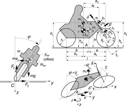
FIGURE 11.1 Motorcycle model configuration.

11.2.1 Geometry and Inertia

The geometrical dimensions of the motorcycle and the location of the centers of gravity of the four connected bodies (mainframe including lower part of the rider and rear wheel, upper torso of the rider, front upper frame, and front subframe including front wheel) are defined by quantities given in the figure. The following relations exist between geometrical parameters:

(11.1)

The last three dimensions have not been indicated in the figure.

The masses of the mainframe, the front upper frame, the front subframe, and the upper torso are denoted as m_m, m_f, m_s, and m_r respectively. The magnitude of total mass m, the possibly shifted c.g. of m_mr = m_m+ m_r, the wheel base l, and the location of the center of the total mass center with respect to the rear and front wheel axles (distances a and b) and above the ground (height h) become:

(11.2)

The inertial quantities (provided with subscript 0) that would apply in case of a rigid rider (lean angle remains zero) may be retrieved by using the following equations where I_rx is the moment of inertia of the rider’s upper torso about its longitudinal axis; I_rz is assumed to be incorporated in the mainframe inertia:

(11.3)

Products of inertia, except I_mxz of the mainframe, will be neglected.

The cross-sections of the tires are assumed to have a finite crown radius r_c₁ and r_c₂ (front and rear). These radii are responsible for the creation of the major part of the tire overturning couples M_x_1,2. Moreover, the heights of the c.g.s are affected by these crown radii when running at large roll angles. Figure 11.2 illustrates such a situation.

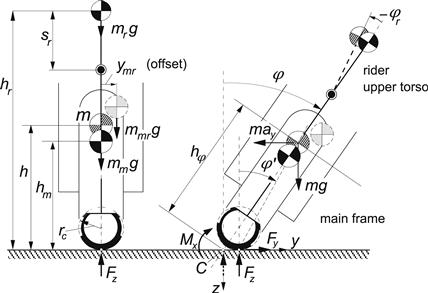
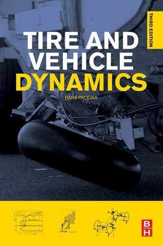
FIGURE 11.2 Rear view of motorcycle with tire cross-section and possible c.g. offset indicated.

Important is the notion of the so-called contact center or point of intersection C that lies below the wheel spin axis and on the line of intersection of wheel center plane and road surface. We may refer to Figure 4.27 and the related discussion. For the rear wheel the center plane coincides with the plane of symmetry of the (assumedly symmetric) mainframe. Rotation of the mainframe about the line of intersection gives rise to an increase of the normal load of the tire. At constant vertical load, a simultaneous lift of the vehicle must occur. Consequently, the distance of the center of gravity to the line of intersection will increase from h to h_φ, as indicated in the figure. With a weighted average crown radius

(11.4)

we find:

(11.5)

At large roll angles also the caster length t_c should be adapted. We find approximately with δ assumed small:

(11.6)

In the linear analysis restricted to small angles, these extensions are of no importance.

11.2.2 The Steer, Camber, and Slip Angles

To determine the side force F_y and the moments M_x and M_z acting on the front and rear wheels, the respective slip and camber angles are needed as input. For the rear wheel these angles can be obtained in a straightforward way. The front wheel poses a problem because we have an attitude of the wheel plane that is defined by at least three successive rotations. In Figure 11.3 several triads have been introduced which are needed to define the orientation of mainframe and front wheel. The line of intersection of the mainframe center plane and the road plane coincides with the x axis. The origin of the horizontal moving axes system (x, y, z) is the reference point A indicated in Figure 11.1 with forward and lateral velocity components u and v. Furthermore, this system rotates about the vertical axis with yaw rate r = . The mainframe rotates about the x axis giving rise to the roll angle φ. The rotated system of axes (x_φ, y_φ, z_φ) is attached to the mainframe. In the mainframe center plane the steering axis is positioned at an angle of inclination (the rake angle ε) with respect to the z_φ axis. The triad (x_ε, y_ε, z_ε) is also attached to the mainframe but with a z_ε axis along the inclined steering axis. The system (x_δ, y_δ, z_δ) is attached to the upper part of the front frame that is rotated with steer angle δ with respect to the (x_ε, y_ε, z_ε) frame. Finally, we may introduce the twist angle β (not shown in Figure 11.3, cf. Figure 11.1) giving rise to the system of axes (x_β, y_β, z_β) with the y_β axis running along the wheel spin axis. We now introduce a unit vector s directed according to the wheel spin axis, that is, along the y_β axis. The components of this vector along the axes of the moving horizontal system (x, y, z) will now be determined by successive rotation transformations. The result of each successive step is indicated by a subscript that denotes the frame with respect to which the unit vector is regarded. We have

(11.7)

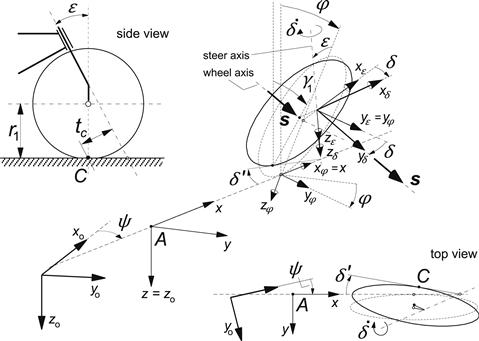
FIGURE 11.3 View of front wheel assembly with various coordinate system triads to assess the ground steer angle δ′ and camber angle γ₁ of the front wheel using the unit vector s along the wheel spin axis (β = 0).

In the subsequent analysis we will approximate the situation by assuming small steer and twist angles. This is certainly admissible. For the non-linear steady-state cornering problem, the roll angle should be allowed to attain magnitudes larger than 45°. Of course, the rake angle ε which is a system parameter will be regarded to be large. With δ and β assumed small, the unit vector reduces to:

(11.8)

which in case of a completely linear analysis, with also the roll angle assumed small, reduces to:

(11.9)

The ground steer angle and the camber angle γ₁ can now easily be determined from the components of the unit vector. We find for the non-linear expressions:

(11.10)

(11.11)

and for the linearized approximations:

(11.12)

(11.13)

For the non-steered rear wheel we simply have a camber angle

(11.14)

The slip angles are assumed to remain small and read at steady-state by considering Figure 11.4:

(11.15)

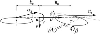
FIGURE 11.4 Top view of the single track vehicle showing the front and rear slip angles.

For the dynamic non-steady-state situation the linearized model will be employed. The slip angles then become, including the time rate of changes of δ and β:

(11.16)

With the camber and slip angles now derived, we can formulate the resulting side force and moments. First, however, the normal loads are to be established. These are affected by the fore-and-aft load transfer caused by aerodynamic drag and braking or driving forces.

11.2.3 Air Drag, Driving or Braking, and Fore-and-Aft Load Transfer

Apart from the forces and moments acting from road to tires, we will consider the aerodynamic drag force F_d that is assumed to act in the longitudinal backward direction in the pressure center a distance h_d above the road surface (in upright position). We will here define the drag force to depend quadratically on the speed u as follows:

(11.17)

Due to the action of the drag force F_d and the longitudinal tire forces F_xi, load transfer arises from the front to the rear wheel. The increase of the rear normal load is (by neglecting the overall aerodynamic lift) equal to the decrease of the front normal load.

The sum of the longitudinal tire forces is denoted as F_x,_tot. The remaining force for the acceleration of the vehicle in longitudinal direction becomes:

(11.18)

which results in the forward acceleration:

(11.19)

and from this, the acceleration forces acting on the four individual masses F_axm = a_xm_m, F_axr = a_xm_r, F_axf = a_xm_f and F_axs = a_xm_s.

With the moment arms h_φ (cf. Figure 11.2) and h_dφ the amount of load transfer becomes:

(11.20)

which for small roll angles reduces to:

(11.21)

The resulting vertical wheel loads now become:

(11.22)

and at small roll angles:

(11.23)

with the initial wheel loads:

(11.24)

The imposed braking force is assumed to be distributed over the front and rear wheels in proportion to the wheel loads as would occur in straight ahead motion, that is: according to the loads (11.23). We have at braking (F_x,_tot < 0):

(11.25)

and at driving:

(11.26)

These forces will act as parameters in the formulae for the tire forces as described in the subsequent subsection.

It may be noted that in the rolled position the longitudinal drag and acceleration forces will also produce a moment about the vertical z axis through reference point A. This gives rise to an increase at the rear and a decrease at the front of the side forces to be generated by the tires almost in proportion to the changes in normal load (not exactly because of the effect of the pneumatic trails). This is essentially different from what happens with the automobile.

11.2.4 Tire Force and Moment Response

Linear Model

We will take into account the transient response of the side force F_y and aligning torque M_z to changes in slip angle and camber angle. However, the non-lagging part of the response will be disregarded. On the other hand, the overturning couple M_x is assumed to respond instantaneously to changes in camber. For the transient responses the relaxation length σ will be used as parameter in the first-order differential equations. These equations describe the responses of the transient slip or deflection angles α′ and γ′ which in steady-state become equal to the input slip and camber angles α and γ. We obtain for tire i (i = 1 or 2):

(11.27)

(11.28)

which gives rise to the side force at small slip and camber angles:

(11.29)

For the aligning torque stiffness against wheel camber we introduce the effect of the longitudinal force F_xi by considering a finite crown radius r_ci assuming that the lateral shift of the line of action of the longitudinal force changes instantaneously with the camber angle. We find for the aligning torque:

(11.30)

Note that we have disregarded here the other influences of the longitudinal force F_xi on the side force and the aligning torque, as expressed e.g. by Eqns (4.45–4.48). To M_z one might add the turn slip moment (5.82) and M_z,gyr (5.178 and 7.49).

Finally, we have the overturning couple indicated in Figure 11.2 assumed here to depend only on the camber angle. In the linearized version we have:

(11.31)

Obviously, we have neglected here the small effect of the lateral distortion due to the side force. The coefficients are assumed to depend on the normal load as follows (omitting subscript i):

(11.32)

(in the linear model d₅ = 0) with

(11.33)

(11.34)

(11.35)

(11.36)

and

(11.37)

We introduce the pneumatic trails t_αo (>0) of the side force due to side slip and t_γo (<0) of the camber force:

(11.38)

Also the relaxation lengths depend on the normal load. This appears to occur in a way similar to that of the change in cornering stiffness. Experimental evidence shows that the relaxation length for side slip is close to the one for camber. The non-lagging part that (although small) exists in the response to camber changes is disregarded here. We define:

(11.39)

Non-Linear Model

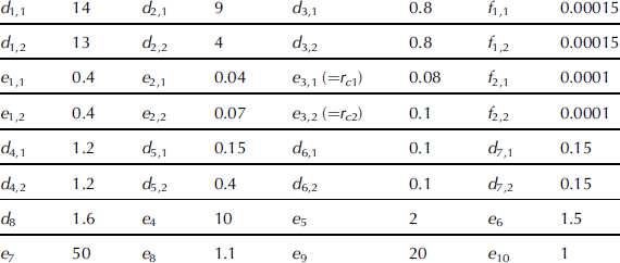
For the non-linear force and moment description we will make use of the Magic Formula in a simplified version. The values of the parameters involved have been listed in Table 11.1. The similarity method will be employed to incorporate the effect of the imposed fore-and-aft force F_x. We will assume here that the cornering stiffness C_Fα is not affected by F_x and that the vertical shift is small with respect to D₀. We have for the side force (again omitting subscript i):

(11.40)

(11.41)

(11.42)

(11.43)

(11.44)

(11.45)

(11.46)

(11.47)

(11.48)

(11.49)

and for the aligning torque using the pneumatic trail and the side force solely due to side slip:

(11.50)

(11.51)

(11.52)

(11.53)

(11.54)

(11.55)

(11.56)

(11.57)

(11.58)

(11.59)

in which the term with the product F_xF_y has been disregarded. Finally, we define for the overturning couple using formula (4.126) while neglecting the vertical and lateral tire deflection:

(11.60)

TABLE 11.1 Parameters of Hypothetical Front (,1) and Rear (,2) Motorcycle Tire Model.

Since the non-linear analysis will be limited to steady-state conditions, the input slip and camber angles α and γ may be used directly instead of the transient angles α′ and γ′.

As an example, in Figures 11.5 and 11.6, the steady-state characteristics for F_y and M_z versus α have been plotted for a number of γ values for the front and rear tires for the two cases: free rolling and braking. The characteristics of the freely rolling tire are similar to the experimentally found curves (extending from −6 to +6 degrees slip angle) reported by De Vries and Pacejka (1998a). The parameter values have been listed in Table 11.1.

The non-linear analysis may be improved by employing the full Magic Formula description as given in Chapter 4. In the present analysis these equations may be used for κ = 0, with the similarity method employed to include the effects of the given longitudinal force F_x. If instead of the force F_x the longitudinal slip κ is imposed or results from wheel rotational dynamics with imposed braking or driving effort, the complete Magic Formula model with combined slip may be used. For the present study this is a less practical option.

In the diagrams of Figures 11.5 and 11.6 the side force curves show a mainly sideways shift at increasing camber angle. The moment curves are moved upward while their shape is changed. The upward shift is a consequence of the spin torque that results from the wheel inclination angle. At braking (Figure 11.6) the aligning torque at camber is considerably increased in magnitude because of the direct contribution of F_x (<0), which is represented in (11.59) by the last term. It is observed that due to the longitudinal force, the maximum level of the side force is reduced.

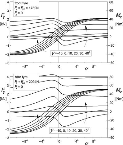
FIGURE 11.5 Side force and aligning torque characteristics for the freely rolling front and rear motorcycle tire model at a series of camber angles.

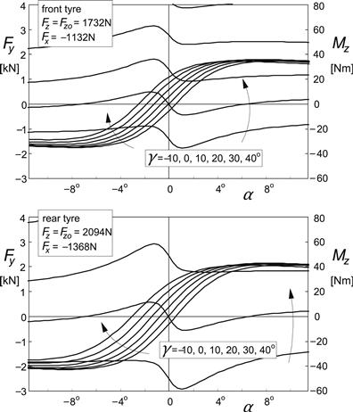
FIGURE 11.6 Side force and aligning torque characteristics for the braked front and rear motorcycle tire at a series of camber angles.

11.3 Linear Equations of Motion

For the dynamic analysis of the vehicle motion we restrict ourselves to small deviations from the rectilinear path. The differential equations will be kept linear with the forward speed u considered as a constant parameter. We will derive the equations using the modified equations of Lagrange (1.28) derived in Chapter 1. After adding the dissipation function D to include damping in the system, these equations read for the variables v and r (=dψ/dt) and subsequently for the remaining generalized coordinates q_j (here: j = 3, 4, 5, or 6):

(11.61)

The generalized forces are found from the virtual work (using Δ instead of δ):

(11.62)

with q_j referring to the quasi coordinate y and to the generalized coordinates ψ, φ, φ_r, δ, and β. To establish the equations we will assess successively the kinetic and potential energies, the dissipation function, and the virtual work. The terms appearing in the resulting expressions will be restricted to terms of the second order of magnitude. The velocity u and the connected wheel speeds of revolution Ω _i = u/r_i, the vehicle weight mg, the aerodynamic drag F_d, and longitudinal force F_x,_tot are quantities of the zeroth order of magnitude whereas the variables v and the generalized coordinates are of the first order of magnitude. Also, the imposed lateral offset y_mr of the combined mainframe and rider mass center is considered as a quantity of the first order of magnitude. Products of first order of magnitude quantities become terms of the second degree. Terms of higher degree will be neglected as these would give rise to second or higher degree terms in the final differential equations, which we intend to keep linear (only first degree terms).

The pitch angle θ of the mainframe which does not represent a degree of freedom is of the second order of magnitude and should be accounted for in the expressions for the energies. Expressed in terms of the generalized coordinates we find the second degree constraint equation, cf. Eqn (11.1):

(11.63)

11.3.1 The Kinetic Energy

Translational and angular velocities of the six bodies are to be expressed in terms of v and the generalized coordinates (and tentatively θ) and their time derivatives. We find for the longitudinal, lateral, and vertical velocities of the c.g. of the mainframe plus rear wheel (except polar moment of inertia I_wy₂) with mass m_m (body1):

(11.64)

and for the angular velocities:

(11.65)

The velocities of the rider upper torso with mass m_r (body 2):

(11.66)

and for the angular velocities:

(11.67)

The velocities of the front frame with mass m_f (body 3 with the z axis parallel to the steer axis):

(11.68)

and

(11.69)

For the front subframe plus front wheel (except polar moment of inertia I_wy₁) with mass m_s (body 4 with the z axis parallel to the steer axis):

(11.70)

and

(11.71)

For the front wheel angular velocities (bodies 5 and 6 only possessing polar moments of inertia I_wy_1,2 possibly extended with effective moment of inertia n_gI_ey of other rotating parts reduced to the wheel rotational speed):

(11.72)

and for the rear wheel:

(11.73)

where

(11.74)

with r₁ and r₂ denoting the front and rear wheel (effective rolling) radii. Due to symmetry of the undisturbed system, the Ω’s do not need to be regarded as variables in our linearized system equations and non-holonomic constraint equations do not occur. The kinetic energy becomes, in general, summed over the six bodies:

(11.75)

The products of inertia will be neglected except I_zx₁ = I_mxz of the mainframe. The velocities u_k, etc. appearing in (11.75) correspond to the quantities given by the expressions (11.64–11.74). The time derivative of the pitch angle θ is obtained from expression (11.63).

11.3.2 The Potential Energy and the Dissipation Function

The potential energy is composed of contributions from torsional spring deflections: twist angle β and lean angle φ_r with stiffnesses c_β and c_φr, respectively, and the heights of the centers of gravity of the various bodies. These heights become expressed in terms of the generalized coordinates and θ:

For body 1 with c.g. lateral offset y_m:

(11.76)

For body 2 with c.g. lateral offset y_r:

(11.77)

For body 3:

(11.78)

For body 4:

(11.79)

Furthermore, we have the torsional deflections φ_r and β. The complete potential energy is now written as follows:

(11.80)

Again, Eqn (11.63) should be employed to express θ, appearing in the formulae (11.76–11.79), in terms of the generalized coordinates.

If we consider viscous damping to be present in the steer bearings and possibly also around the lean and twist axes we obtain for the dissipation function with k_δ, k_φr, and k_β denoting the respective damping coefficients:

(11.81)

11.3.3 The Virtual Work

Through the virtual work the generalized forces each associated with a generalized coordinate can be assessed. The forces which act from the environment upon the vehicle are the horizontal ground forces and moments, the aerodynamic forces, and the gravitational force component in the longitudinal direction in case of a forward slope or the dynamic longitudinal d'Alembert forces acting in the mass centers which are in equilibrium with the longitudinal forces generated by the tires. The option of considering a forward slope that at given aerodynamic drag and driving or braking forces is just able to maintain a constant forward velocity would make the analysis correct as in that case the coefficients of the linear equations are time independent (cf. Eqn (3.123) with (3.126) where this is not the case). The longitudinal acceleration a_x appearing in the ensuing equations may be considered equal to the longitudinal component of the acceleration due to gravity that would arise if the vehicle continuously runs over a road with equivalent forward slope.

With the various forces and moments that act upon the vehicle in and around the respective points of application the virtual work becomes:

(11.82)

The virtual displacements expressed in terms of the generalized coordinates turn out to read:

(11.83)

where Δθ can be expressed in the generalized coordinates by taking the variation of θ (11.63).

Now, we may compare (11.82), after having substituted herein the expressions (11.83), with the formulation of the virtual work according to Eqn (11.62), which becomes:

(11.84)

As a result, the generalized forces Q_j are obtained which are to be inserted at the right-hand sides of the Lagrangean Eqn (11.61).

11.3.4 Complete Set of Linear Differential Equations

All the necessary preparations to set up the equations have been completed. To establish the equations, the operations with the energies as indicated in (11.61) can now be carried out. The resulting set of equations are completed with the four first-order differential equations for the transient slip and camber angles front and rear and the linear equations for the side forces, the aligning torques, and the overturning couples together with expressions of the slip and camber angles all resulting from the analysis of Section 11.2. Note that the tire model coefficients, C_Fα₁, σ_α₁, etc., depend on the current vertical wheel load F_zi = F_zi_o, Eqns (11.23, 11.33–11.39). The total order of the system turns out to be 14.

With a given speed of travel u and the total longitudinal tire force F_x,_tot, the air drag F_d, the vertical tire loads F_z₁₀ and F_z₂₀ and the individual longitudinal tire forces F_x_1,2 can be assessed using the Eqns (11.17–11.19, 11.21, 11.23–11.26). The initial wheel loads (at stand-still) F_z_1o and F_z_2o are directly associated with the vehicle mass distribution, Eqn (11.24). In the equations the imposed handlebar torque M_δ and lean torque M_φr appear in the right-hand members. The tire side forces and moments are tentatively put on the right-hand side as well. In the equation for the steer angle the control terms have been added.

The equations successively for the variables v, r, φ, φ_r, δ, β, , , , and become as follows

(11.85)

(11.86)

φ:

(11.87)

φ_r:

(11.88)

δ:

(11.89)

β:

(11.90)

transient slip and camber angles:

(11.91)

(11.92)

(11.93)

(11.94)

tire forces and moments (coefficients depend on wheel load (11.23, 11.33–11.39)):

(11.95)

(11.96)

(11.97)

(11.98)

(11.99)

(11.100)

slip and camber angles:

(11.101)

(11.102)

(11.103)

(11.104)

the rider feedback control gains, occurring in Eqn (11.89), depend on the speed of travel u and are assessed here by trial and error:

(11.105)

The steer torque M_δ is considered to act in addition to the stabilization steer torque, that results from feedback control, and is represented by the terms containing the control gains in Eqn (11.89).

For the mass center lateral offset we have introduced for abbreviation:

(11.106)

If the steer and roll angles remain sufficiently small so that it may be assumed that geometric linearity still prevails we may investigate the influence of larger wheel slip by using for the tire side forces and moments the non-linear functions of , wheel load F_zi, and the braking/driving force F_xi according to the Eqns (11.40–11.60).

For the baseline configuration of the linear vehicle model the rider is considered rigid (c_φr → ∞). With the rider upper torso released, the parameter values of Table 11.2 hold. The tire parameter values have been chosen as listed in Table 11.1. The model configuration may be considered as typical for a heavy motorcycle. When a rigidly connected rider upper torso is considered (baseline configuration with φ_r = 0), the relevant parameters result from Eqns (11.3).

TABLE 11.2 Parameters of Vehicle in Baseline Configuration but with Rider Upper Torso Released (in Baseline Configuration c_φr → ∞). Rider Control Gains g with Cross-over Velocity u_c

For the linear system defined, the eigenvalues and the steady-state steer angle and steer torque per unit path curvature have been established for a series of values of the speed of travel u (=V). In addition, a number of parameters related to both the vehicle construction and the tires have been changed in value to examine their influence.

11.4 Stability Analysis and Step Responses

11.4.1 Free Uncontrolled Motion

In a series of diagrams the variation of the eigenvalues as a function of speed has been presented. The diagram of Figure 11.7 represents the situation corresponding to the baseline configuration defined by Tables 11.1 and 11.2 but with the rider regarded as a rigid element of the mainframe body. The upper diagram gives the real part of the eigenvalues of this 12th order system versus speed indicating the degree of instability (if positive) or damping (stable, if negative). The second diagram presents the variation of the imaginary part of the eigenvalues that represent the frequencies of the different modes of vibration (in rad/s). The third diagram depicts the variation of the eigenvalues in the complex plane. Along the curves the speed changes as indicated.

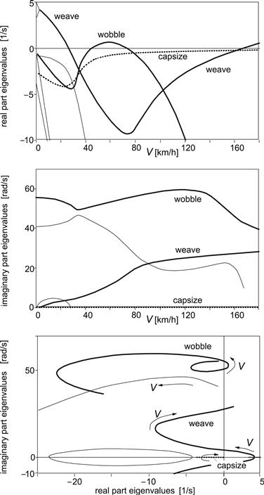
FIGURE 11.7 Baseline configuration (rigid rider, with air drag, zero forward acceleration, no control). Real and imaginary parts of eigenvalues versus speed of travel V.

The weave mode is a relatively low-frequency oscillatory motion in which the whole vehicle takes part. This mode exhibits a possibly dangerous unstable yaw and roll motion at higher speeds (in our case above a speed of ca.165 km/h) with a frequency of 3 to 4 Hz. At low speeds the frequency decreases and the mode becomes unstable and constitutes the phenomenon where the uncontrolled vehicle falls over.

At very low speed it is observed that the complex pair of roots with a positive real part changes into two positive real roots constituting the divergent unstable modes associated with capsizing of the whole machine and of the front frame about the inclined steer axis (the latter is observable with the motorcycle on its center stand and with the front wheel clear of the ground). The frequency of the oscillation can be found from the two lower plots. In the high speed unstable range the frequency of the weave mode appears to be around 27 rad/s or ca. 4 Hz.

The capsize mode can in certain cases become (moderately) unstable beyond a relatively low critical velocity. The eigenvalue remains real and, consequently, the motion does not show oscillations. In our case, this mode remains stable. The third mode that is of interest is the wobble mode, which is a steering oscillation that can become unstable in a range of moderate speeds (in our case between ca. 45 and 70 km/h). The frequency in the unstable range appears here to take values around 55 rad/s or ca. 8 Hz as can be seen in the two lower plots with the imaginary part as the ordinate. The frequency is mainly influenced by the front frame inertia, the mechanical trail, and the front tire cornering stiffness. The remaining modes are well damped and consequently of less interest.

Starting out from the baseline configuration (with air drag) the effect of changes in several system parameters has been investigated. To get a clear picture of the role various parameters play in stabilizing or destabilizing this single track vehicle, their values have been changed drastically. Figure 11.8 shows the resulting stability characteristics. For clarity, the weave, capsize, and wobble mode curves have been shown in separate diagrams. From the results we may conclude the following:

1. The model shows that absence of air drag (case 1) slightly stabilizes the weave mode and destabilizes the wobble mode.

2. Torsional rigidity of the mainframe (case 2, large c) appears to be of crucial importance especially for the manner in which the wobble manifests itself. High stiffness or disregarding the torsional compliance gives rise to a (too) high critical speed. A more flexible frame (baseline configuration) causes the wobble to occur in a limited range of speed around 50 km/h, which turns out to be experienced also in reality.

3. Almost vanishing relaxation lengths (rapid tire response) drastically suppresses the wobble instability.

4. Making the tire almost rigid (with in addition to very small σ: very large cornering stiffness and very small pneumatic trail, case 4) would drastically suppress the high speed weave but gives rise to violent wobble over a large range of speed. Much larger camber force stiffness cannot be technically realized even with a very stiff solid wheel. It would increase the low speed unstable weave range and stabilize the high speed weave; wobble is almost not affected (not shown).

5. Making only the aligning torque stiffnesses very small destabilizes the high speed weave mode and stabilizes the wobble mode. The capsize root is made more negative.

6. Even a considerable decrease of the camber aligning moment stiffness has very little effect, at least in the case of zero or very small longitudinal tire forces. The same holds for the overturning couple stiffness, that is: a small crown radius (not shown). The smaller camber aligning moment stiffness does have an influence on the capsize stability. As indicated in the diagram, capsize instability now shows up and occurs beyond a speed of around 20 km/h.

7. The fundamental role of the gyroscopic coupling terms becomes evident when the polar moments of the wheel are considerably reduced (case 7). First, the low speed unstable weave range is stretched to almost 70 km/h and second, the wobble becomes violently unstable up to very high levels of speed. It may be concluded that the gyroscopic effect of the rotating wheels is largely responsible for the fact that the motorcycle is capable of moving in a stable manner.

8. Reduction of the rake angle to an almost vertical steer axis orientation with the caster length kept the same would strongly destabilize the wobble mode.

9. At the same time reducing the caster length as well (case 9) would strongly destabilize the weave mode, which unveils the fundamental effect of introducing the steer axis backward inclination.

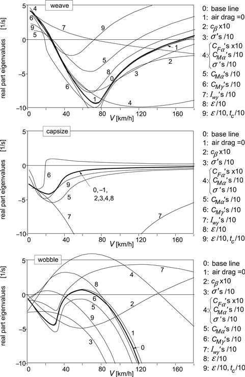
FIGURE 11.8 Effect of drastic changes in model parameter values on stability characteristics.

Effects of more realistic levels of variation of the system parameters have been presented in the stability diagrams of Figure 11.9. Comparison with the curves that represent the baseline configuration (0) reveals that (again, curve numbers correspond to list numbers below):

• A 20% smaller front relaxation length stabilizes the wobble mode and has practically no effect on the weave and capsize modes.

• A smaller rear relaxation length stabilizes the wobble mode to a lesser degree and stabilizes the weave mode. No effect on the capsize mode.

• Moving the center of gravity of the mainframe plus rider 10 cm forward turns out to strongly stabilize the weave mode. However, it destabilizes the wobble. Capsize is not affected.

• Lowering both center of gravity over 10 cm stabilizes both the weave and wobble modes a little. The capsize mode becomes more stable.

• Adding steer damping does, of course, stabilize the wobble mode. However, it adversely affects the weave mode stability.

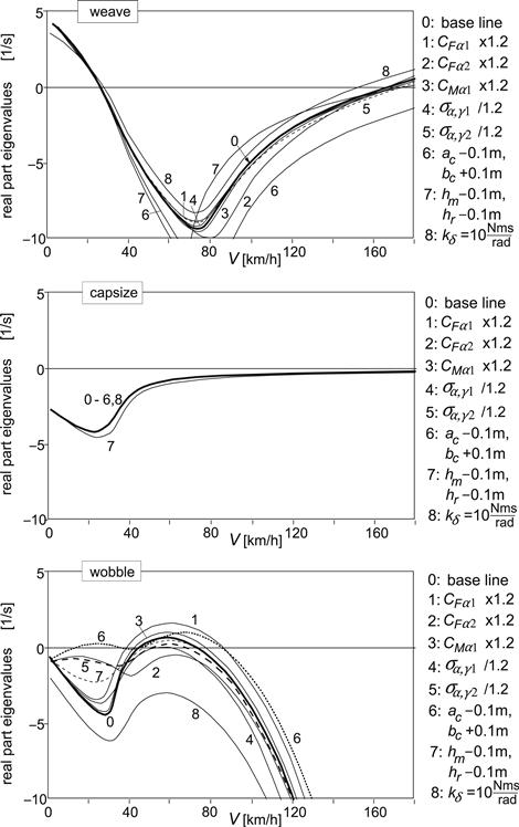
FIGURE 11.9 Effect of realistic changes in parameter values on stability characteristics.

For the free control situation, we finally consider the influence of driving or braking and the addition of a degree of freedom: the rider lean angle measured with respect to the mainframe roll angle.

Figure 11.10 shows the stability diagram of the baseline configuration at zero net acceleration force (11.18) when F_ax = 0 (rear wheel driving force just withstands the air drag so that speed is constant), at braking (11.25) F_ax = –1500 N, and at driving (11.26) F_ax = 1500 N. It is observed that braking destabilizes the wobble mode, which is mainly due to the increased normal load at the front wheel that gives rise to larger relaxation length and cornering and aligning stiffnesses, the effects of which were shown in Figure 11.9. The terms with F_x₁ δ in Eqn (11.86) (destabilizing) and with h_β F_x₁ β in Eqn (11.89) (stabilizing) have a smaller effect. The terms in Eqns (11.85) and (11.89) with F_x₁ appear to largely neutralize the stabilizing effects of the increased front wheel load.

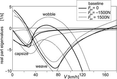
FIGURE 11.10 Effect of the application of braking (F_ax, F_x_1,2 < 0) and driving forces (F_ax, F_x₂ > 0) on the stability diagram (baseline configuration).

When driving, the longitudinal force is generated at the rear wheel only. Obviously, wobble is completely suppressed. Weave, however, appears to show up already at considerably lower speeds.

As depicted in Figure 11.11, the introduction of the lean angle of the rider as an additional generalized coordinate with torsional stiffness and damping with respect to the mainframe gives rise to a decrease of the critical velocity for weave instability while the wobble mode is hardly affected. The lean angle is introduced to enable the study of the response of the vehicle motion to a step change in lean torque M_r, which is defined to act between the upper torso and the mainframe about the longitudinal lean axis.

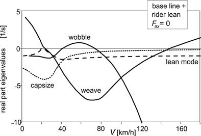
FIGURE 11.11 The stability diagram with the rider lean degree of freedom introduced.

11.4.2 Step Responses of Controlled Motion

We will study the responses of the vehicle motion to a unit step of the imposed steer torque M_δ and of the lean torque M_r. This, as a first attempt to investigate the transient handling quality of the vehicle. First, the motorcycle must be stabilized in the range of speed we want to cover. For this, the various feedback signals have been provided with gains defined by Eqn (11.105) and Table 11.2. In Figure 11.12 the six gains have been presented as a function of the speed of travel. Similar functions have been used by Ruijs (1985) in the feedback control loops to stabilize the unmanned motorcycle with a stabilizing rider-robot. The peculiar change in sign that occurs in the gain from roll rate to steer torque is essential to stabilize both the low- and the high-speed weave.

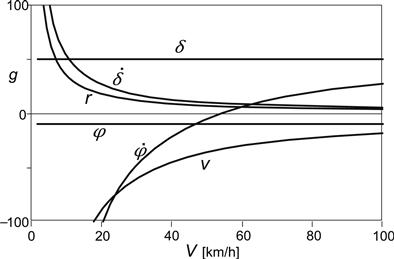
FIGURE 11.12 Hypothetical rider steer torque feedback stabilizing control gains versus speed.

The resulting stability diagram is presented in Figure 11.13. Comparison with Figure 11.10 shows that adopted feedback gains considerably enlarge the stable velocity range, especially at the low end. An additional control action using the lean torque (and as a consequence moving the rider c.g. laterally) would be necessary to further push back the low speed instability which here appears to correspond to an unstable lean mode. At such low speeds, steering would be almost ineffective to move the contact point laterally and thereby stabilize the motion.

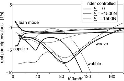
FIGURE 11.13 The stability diagram with feedback steer torque control of Figure 11.12 activated.

In Figure 11.14 the resulting unit step responses have been shown for the case of zero F_ax. The figure depicts the variations of the yaw rate r, the steer angle δ, the mainframe roll angle φ, and the upper torso roll angle φ + φ_r. Two values of speed have been considered: 35 and 70 km/h. The results are most interesting. We observe that, as a result of a positive change in steer torque (to the right), first a positive steer angle arises with also positive yaw rate (to the right). After a short time, a change in sign occurs and a negative yaw rate is being developed with a negative steer angle. It is seen that during this short transition time the roll angle begins to build up in the correct direction (to the left) that belongs to the final steady-state curving situation. This variation in the motion variables is similar to what would be observed in reality. The uncontrolled vehicle is stable at the speed V = 35 km/h (Figure 11.11). If at this speed the stabilization controller would not be activated, the motorcycle exhibits a similar response but with angles and yaw rate becoming larger and with less damped wobble and weave vibrations.

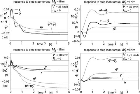
FIGURE 11.14 The step responses of motion variables to unit steer and rider lean torque at zero forward acceleration, F_ax = 0 (with rider stabilizing control).

The lean torque response shows initially a negative roll angle, which is the result of counteracting the imposed (internal) lean torque. After the initial phase, the angle becomes positive. Also the steer angle and with that the yaw rate turn out to become negative in the initial phase which causes the contact points to move in the right direction (to the left). The steady-state situation is reached after low-frequency damped lean mode oscillations. If the controller is not activated, a very similar response with now low-frequency damped weave oscillations (Figure 11.11) occurs. Now, it becomes clear that it is mainly the gyroscopic couple (plus camber aligning moment) that steers the front wheel initially in the right direction. Analysis shows that the hardly visible small, positive, steer angle peak right after the lean torque step change is due to the mechanical trail and the aligning stiffness of the front wheel (t_c and C_Mα₁).

At the higher speed of V = 70 km/h the responses show the same tendencies but with much smaller steer angles and yaw rates. The weave is more damped and the wobble less. Without the controller the wobble becomes unstable and a violent steering oscillation at ca. 9 Hz is developed.

With the lean degree of freedom disregarded, only the response to steer torque can be considered. The resulting motion responses turn out to get close to those depicted in the left-hand diagrams of Figure 11.14 with the curves for φ + φ_r deleted. The low-frequency oscillation that is predominant at the lower speed is now attributed to the weave mode. The uncontrolled system (Figure 11.7) is just stable at 35 km/h and behaves similar to the controlled one albeit that a somewhat larger weave and wobble vibrations and a larger steady-state response arise. At 70 km/h the unstable wobble vibration develops again.

Figure 11.15 presents the results for the system while the brakes are applied (F_ax = –1500 N). The course of the various signals show similar tendencies as occurs in the unbraked situation. The obvious differences are the lowly damped wobble vibration that is seen to occur at 70 km/h (cf. Figure 11.13) and the much smaller steady-state responses (cf. Figure 11.20 of next section). These differences are primarily due to the accompanied load transfer.

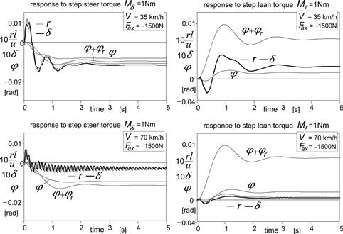
FIGURE 11.15 The step responses of motion variables to unit steer and rider lean torque while braking, F_ax = – 1500N (with rider stabilizing control).

11.5 Analysis of Steady-State Cornering

When a steady-state cornering condition is reached equilibrium of forces and moments exists. We consider the equilibrium in lateral direction, about the vertical axis, and about the line of intersection of the mainframe center plane and the road plane, this in addition to the static equilibrium of forces in the vertical direction. In the approximate analysis the small c.g. forward offsets of the steerable front and subframes e_f and e_s will be neglected. In addition, the twist angle β and the rider lean angle φ_r will be disregarded. Instead, we will study the effect of a sideways shift y_mr of the center of gravity of the combined mainframe and rider. Once the side forces and the roll angle have been assessed at a given lateral acceleration, the slip angles can be determined, and from their difference with the given non-dimensional path curvature, l/R, the steer angle can be estimated. By considering the equilibrium about the steering axis the steer torque needed to maintain the curving motion is derived.

First, an approximate linearized theory is developed. The findings will be compared with the exact steady-state solutions of the linear differential Eqns (11.85)–(11.94) with the φ_r degree of freedom deleted. After that, the theory is extended to larger roll angles and the non-linear handling diagram is established for the steadily cornering motorcycle.

11.5.1 Linear Steady-State Theory

The theoretical expressions for the coefficients concerning the steady-state turning behavior and the c.g. lateral offset effects will be developed in several successive stages starting with the simplest case in which tire moments, gyroscopic effects, and air drag are disregarded and ending with the ultimate configuration in which all these items are included and driving or braking may be considered. First, the required roll and steer angles will be assessed and, with these results, the expression for the steer torque determined.

Wheel Moments and Air Drag Neglected

As an introduction, we will first discuss the simple case where the air drag, longitudinal tire forces, and all the tire moments about the vertical axis are disregarded. That means that the aligning moment, the overturning couple, and the spin (camber) moment are set equal to zero. Moreover, we neglect the gyroscopic couples.

For the lateral wheel forces we find as in Chapter 1, Subsection 1.3.2, Eqn (1.61) for the automobile with pneumatic trails neglected (equilibrium in the lateral direction and about the vertical axis)

(11.107)

The roll angle φ_y needed to maintain equilibrium about the longitudinal x axis when a lateral offset y_mr of the center of gravity of the combined mainframe and rider exists (cf. Figures 11.1 and 11.2) equals

(11.108)

The additional roll angle of the motorcycle that arises while cornering becomes

(11.109)

The front and rear camber angles read in terms of the roll angle and the ground steer angle, cf. Eqns (11.12)–(11.14):

(11.110)

(11.111)

The slip angles result from Eqn (11.29), primes omitted, with (11.107–11.111). We find:

(11.112)

(11.113)

These equations show the importance of the difference between camber stiffness (N/rad) and initial tire load (N) in view of the sign of the slip angles. Obviously, in general, side slip is needed to accomplish lateral/yaw equilibrium. It may be realized that at higher speeds the steer angle is much smaller than the roll angle,

With the wheel base l = a_c + b_c and the Eqn (11.15) we find the relationship between the ground steer angle on the one hand and the non-dimensional path curvature l/R = lr/u and the difference of slip angles on the other:

(11.114)

With the use of (11.112 and 11.113) the ground steer angle may now be written in terms of the non-dimensional path curvature l/R, the lateral acceleration a_y, and the c.g. offset y_mr:

(11.115)

where we have introduced the steer angle coefficient ζ which is a bit larger than unity:

(11.116)

the understeer coefficient η of the simplified system,

(11.117)

and the c.g. offset coefficient η_y,

(11.118)

Since we have proportions occurring in the right-hand member of (11.117) which are all of the same order of magnitude it is evident that the understeer coefficient of the single track vehicle is quite different from its counterpart that is found for the automobile where only the first two terms appear in the simplified analysis while ζ is assumed equal to one. The ratio of camber and cornering stiffness front relative to rear is of decisive importance for the sign and magnitude of the understeer coefficient and consequently also for the difference in slip angle front and rear which follows from (11.114 and 11.115):

(11.119)

where the first term in the right-hand member vanishes if the rake angle equals zero making ζ = 1.

When the motorcycle moves straight ahead (l/R = a_y = 0) Eqns (11.115 and 11.119) show that a steer angle and difference in slip angles would arise solely as a result of the c.g. offset and depend on the difference of the ratios of camber and side slip stiffnesses front and rear.

The general course of steer angle and roll angle versus speed of travel at a given path curvature and c.g. lateral offset has been illustrated in Figure 11.16. The coefficients ξ; and ξ;_y will be defined below.

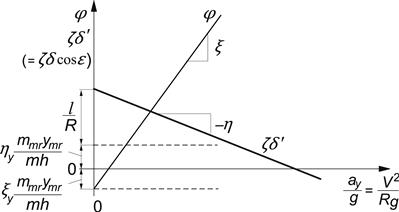
FIGURE 11.16 The ground steer angle δ′ and the roll angle φ due to path curvature 1/R and c.g. lateral offset y_mr and the variation with lateral acceleration a_y.

The actual steer angle δ of the handlebar about the inclined steer axis with rake angle ε is obtained from the ground steer angle δ′ by dividing this angle by cos ε as has been formulated by Eqn (11.12) with twist angle β set equal to zero.

If fore-and-aft load transfer due to aerodynamic drag is considered, the lines of Figure 11.16 are not quite straight anymore. The understeer coefficient η corresponds to the slope of the line in the diagram if air drag is neglected. This may be compared with the theory for the automobile where ζ is taken equal to unity and air drag is disregarded (Figure 1.10). If, at high speed, air drag is not negligible, η is found as the slope of the characteristic that arises if ζδ′ – l/R is plotted against a_y/g with the speed V held constant while the curvature increases with growing lateral acceleration. If we would plot ζδ′ versus a_y/g, again, in this linear theory with constant speed, a straight line arises which now has a slope equal to lg/V² + η. For the sake of convenience the above definition for the degree of understeer has been adopted although a more proper definition might be η′ = (∂ δ / ∂(a_y/g))_R = (η/ζ)/cos ε.

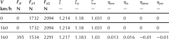
Discussion of numerical results (Table 11.3) follows after more adequate approximations have been developed. For the simple theory developed so far the coefficients ξ; and ξ;_y appearing in the diagram are equal to unity. Below, we will see the effect of tire width and gyroscopic couples on these roll angle coefficients.

TABLE 11.3 Handling Coefficients with Tire Aligning Moments Neglected. F_z_1o = 1732N, F_z_2o = 2094N, cos ε = 0.878; Eqns (11.116–11.118 and 11.123–11.129)

Tire Overturning and Gyroscopic Couples Included

Closer consideration of the roll equilibrium around the line of intersection reveals that instead of (11.109) we actually have with also the caster length t_c taken into account (cf. Eqn (11.87) with (11.2)):

(11.120)

The third term represents the sum of gyroscopic couples. With Eqns (11.13), (11.14) and (11.31), we obtain for the roll angle:

(11.121)

Inspection of the values of parameters as listed in Tables 11.1 and 11.2 leads to the conclusion that the steer angle δ has a negligible effect on the relationship between roll angle φ and y_mr and also between φ and lateral acceleration a_y = ur if δ ∼30(a_y/g). With δ expressed in radians it is expected that at not too low speed, this condition will soon be satisfied in the more interesting range of operation.

We will henceforth use the approximate expression for the roll angle with the δ term in (11.121) neglected:

(11.122)

where the tilt coefficients ξ; and ξ;_y read:

(11.123)

(11.124)

The quantities appear to be a little larger than unity due to the gyroscopic action and the width of the tires (finite crown radii). The tilt coefficients become in the baseline configuration (Tables 11.1 and 11.2):

(11.125)

An effective tilt angle (the angle of the dashed line, through tire contact point and mass center, indicated in Figure 11.1 with respect to the vertical) may be defined. We have:

(11.126)

With the additional moments about the x axis now introduced, we find for the understeer coefficient:

(11.127)

and the c.g. offset coefficient:

(11.128)

while the steer angle coefficient ζ remains unchanged:

(11.129)

The numerical values listed in Table 11.3 will be discussed later on.

Tire Yaw Moments Included

Because of the obvious sensitivity to slight variations in tire parameters we should examine the influence of the remaining (yaw) moments due to side slip and camber acting on the tire. When taking into account the tire aligning torques and the moment applied by the air drag force (assumed to act parallel to the x axis) we find for the tire side forces from the equilibrium conditions:

(11.130)

(11.131)

in which the lateral acceleration a_y can, with (11.122), be expressed in terms of the roll angle φ and the c.g. offset y_mr. The aligning torques are

(11.132)

with camber aligning torque stiffness that without the action of the longitudinal tire force is defined by (11.36). The camber angles can be expressed in terms of the roll angle and the slip angles by using the relations (11.109, 11.110, and 11.113). We have:

(11.133)

(11.134)

From the thus created two equations the two unknown slip angles α_i can be solved and expressed in terms of the known path curvature l/R, roll angle φ, and c.g. offset y_mr. By substituting the expression (11.114):

in the relationship (11.115):

and using again (11.122) the steer angle, understeer, and c.g. offset coefficients ζ, η, and η_y can finally be assessed. The resulting expressions read:

(11.135)

with the effective wheel base

(11.136)

and

(11.137)

and

(11.138)

in which the coefficients λ₁ and λ₂ have been introduced:

(11.139)

(11.140)

which are close to unity (around 1.03 and 0.95, respectively, in the baseline configuration changing a little depending on load transfer).

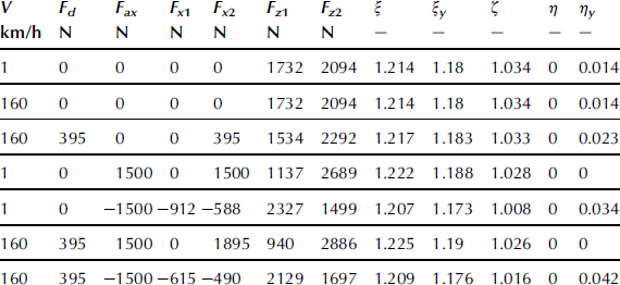
In Table 11.4, the values that η and η_y take in the baseline configuration (Tables 11.1 and 11.2) for the cases without and with air drag (in the latter case at speeds 1 and 160 km/h) have been listed together with the current wheel loads and air drag force.

TABLE 11.4 Handling Coefficients with Aligning Moments and Driving and Braking Included. F_z_1o = 1732N, F_z_2o = 2094N, cos ε = 0.878; Eqns (11.123), (11.124), (11.135)–(11.138), (11.144)–(11.146)

Driving and Braking Forces Included

Applying longitudinal forces to the tires through braking or driving have three effects on the handling behavior of the vehicle occurring through the tires. First, we have the direct effect (only at braking) due to the sideways component of the front wheel longitudinal tire force that arises as a result of the steer angle. Then, we have two indirect effects brought about by changes in tire behavior due to the longitudinal force (notably in the camber aligning torque coefficient C_Mγ), and due to the induced load transfer. In addition, the longitudinal acceleration inertia forces acting at the mass centers exert a moment about the vertical z axis if we have a roll angle φ and possibly a c.g. lateral offset y_mr. The front and rear lateral tire forces now become, instead of the right-most members of Eqns (11.130) and (11.131),

(11.141)

(11.142)

with the tire aligning torques according to (11.132) but with the total camber aligning torque stiffness now expressed as (according to (11.30)):

(11.143)

The same procedure is followed as before and we find the coefficients ζ, η, and η_y augmented for the presence of vehicle acceleration a_x and longitudinal tire forces F_x₁. The terms that are to be added to the expressions (11.135, 11.137, and 11.138) (for zero acceleration, F_ax = 0, cf. (11.19)) read respectively:

(11.144)

(11.145)

(11.146)

Numerical Results

For the parameter values of the baseline configuration the various handling coefficients have been presented in Tables 11.3 and 11.4 together with the calculated air drag, wheel loads, and possibly braking or driving forces (for a given acceleration force F_ax).

Table 11.3 shows the values obtained when using the simpler expressions for the coefficients which result when the gyroscopic and overturning couples and/or the aligning torques are neglected, according to the theories covered by the Eqns (11.107–118) and (11.120–11.129). The influence of air drag results here from the induced load transfer. Table 11.4 presents the results when all the moments are accounted for and also braking and driving may be considered. The equations concerned are (11.130–140) and (11.141–146). First of all, when we compare the different stages of approximation, it is observed that the influence of the various wheel and tire moments is essential in generating more correct values of understeer and c.g. offset coefficients, η and η_y.

The steer angle coefficient ζ is much less affected by the tire moments while the roll angle coefficients ξ; and ξ;_y are influenced considerably by the gyroscopic and/or overturning couple coefficients; note that these coefficients take the value one in the simplest approximation according to Eqns (11.108 and 11.109).

The last two columns of Table 11.4 indicate that, for the conditions considered, the understeer coefficient shows large changes but keeps the same negative sign, which means: steering less to the right for a right-hand turn if speed is increased. In automobile terms one would speak of an oversteered vehicle. However, the steer angle does not serve as an input quantity and the speed where the steer angle changes sign is not a critical speed beyond which instability occurs. It is the steer torque that acts as the input variable and when at a given path radius a change in sign of the steer torque would arise at a certain velocity, the system becomes unstable because in that situation the last term of the characteristic equation of the system becomes negative. We then have divergent instability corresponding to the capsize mode that becomes unstable beyond a critical speed as illustrated in the diagram of Figure 11.8, case 6, with very small camber aligning stiffness.

The sign of the c.g. offset coefficient appears to change from positive to negative in the case of accelerating at low speed. When the rider hangs to right-hand side (y_mr > 0 making φ < 0) while moving straight ahead, steering to the right is normally required to compensate for the camber forces pointing to the left. This appears to be true except when the rear wheel driving force produces sufficient positive yaw moment through the finite crown radius.

As was already clear from the relevant expressions, the influence of speed on the coefficients occurs if air drag is included in the model. At the high speed of 160km/h the effect of air drag becomes quite noticeable. This would be much less at a speed of say 100km/h because of the quadratic speed influence.

As was to be expected, the longitudinal tire forces have a large effect on the two coefficients. When driving with F_ax = 1500 N, coefficient η changes from −0.0177 to −0.0204. At the high speed, much more driving force at the rear wheel is needed to overcome the air drag and realize the aimed acceleration. Oversteer has increased a lot with respect to the situation at zero acceleration (first and third row). The driving force and the opposite inertia force form a couple around the vertical axis (because of the roll angle) that tries to turn the vehicle more into the curve. At braking, more understeer arises caused by the forward inertia force exerting an outward couple about the z axis and the sideways component of the front wheel braking force that does the same, trying to straighten the vehicle's path.

As an example, we might further analyze the case represented by the last row of Table 11.4. If the motorcycle would be negotiating a circular path with a radius of 200 times the wheel base, l/R = 0.005, and R = 300 m, at V = 160 km/h (=44.4 m/s) the lateral acceleration becomes a_y = V²/R = 6.58 m/s² = 0.67 g. As a consequence, the roll angle becomes φ = ξ; a_y/g = 1.209 × 0.67 = 0.81rad = 46°. The ground steer angle takes the value: δ′ = (l/R + ηa_y/g)/ζ= –0.0027/1.016 = –0.00266 rad = –0.15° and the handlebar steer angle δ = δ′/cos ε =– 0.17°. It is obvious that with this high lateral acceleration the assumption of linearity is not valid. A smaller path curvature would have been a better choice. If the center of gravity of the mainframe plus rider is located a distance y_mr = 1 cm to the right of the vehicle center plane, a roll angle φ = –ξ;_ym_mry_mr/mh = –1.176 × 350 × 0.01/(390 × 0.59) = –0.018 rad = –1.03° results at straight line running. The ground steer angle is predicted to amount to δ′ = η_y m_mry_mr/mh = 0.0423 × 350 × 0.01/(390 × 0.59) = 6.38 × 10⁻⁴ rad = 0.036°and the handlebar steer angle δ = 0.041°. In Figures 11.17 and 11.18 this case where the brakes are applied is further examined for speeds ranging from 1 to 100 km/h, also showing the variation of the slip angles.

In Figure 11.17 the left-hand diagram is presented for the non-accelerating vehicle with air drag included (rows 1 and 3 of Table 11.4) showing the variation of the roll angle and the ground steer angle vs speed squared. In addition, the variation of the front and rear slip angles has been depicted. The almost straight lines result from computations with the steady-state version of the differential Eqns (11.85–11.94) with the rider lean degree of freedom deleted. An additional (dotted) line shows the variation of the ground steer angle according to the approximate analytical results corresponding to those listed in Table 11.4. Only very slight differences appear to occur between the approximate (β disregarded and the δ term in Eqn (11.121) neglected) and exact results for the ground steer angle, slip angles, and roll angle. According to the exact computations, the twist angle β amounts to ca. 0.5% of the roll angle φ. Note that the difference in slip angles α₂ − α₁ practically equals l/R minus the ground steer angle δ′ (ζ being very close to unity). We may calculate the slip angles following the analytical approach through an explicit expression by using the Eqns (11.148) and (11.149) for the lateral tire force components caused by side slip, given later on.

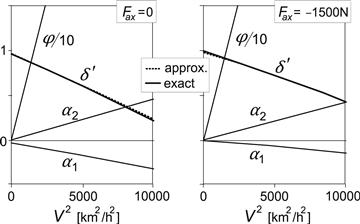
FIGURE 11.17 Steer, roll, and slip angles per unit non-dimensional path curvature l/R versus speed squared V² = a_yR (left: non-accelerating, right: braking) according to the exact and approximate theories.

The right-hand diagram of Figure 11.17 refers to the situation that arises when the brakes are applied (fifth and last row of Table 11.4). Again, an excellent correspondence between the approximate and exact solutions occurs. Obviously, the vehicle performs now in a less oversteered manner as was already concluded from the less negative value of η in Table 11.4. The front slip angle is less negative to make the side force more positive to counteract the sideways component of the front wheel braking force. At the same time, the rear slip angle is made slightly larger to help compensate for the positive yaw moment that arises from the braking forces, their points of application being shifted to the right because of the finite crown radii. Under this condition of braking, β appears to become somewhat smaller.

Finally, Figure 11.18 shows the variation of the various angles per unit lateral c.g. offset. It is seen that the influence of speed is very small and that the agreement between approximate and exact results is good. Both slip angles are positive thereby neutralizing the camber forces which point to the left because of the negative roll angle that arises to compensate for the c.g. location lateral offset. At braking, the center of gravity remains above the line connecting the contact points of the tires. The forward load transfer reduces the rear camber force, which allows a decrease of the rear slip angle. As α₁ increases only a little to balance both the increased camber force and the sideways component of the front wheel braking force, the steer angle needs to become larger to keep α₁ − δ′ equal to α₂. In both cases, β is equal to ca. 5% of φ and will have a relatively large effect on the actual value of steer angle of the handlebar δ (cf. Eqn (11.12)).

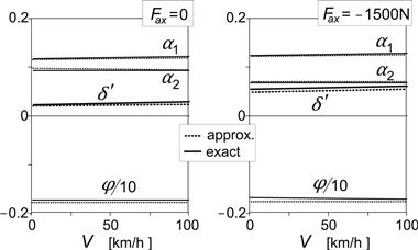
FIGURE 11.18 Steer, roll, and slip angles per m lateral c.g. offset y_mr that occur at straight line motion (according to the exact and approximate theories).

The Steer Torque

By considering Eqn (11.89) with β neglected the following steady-state expression for the steering couple is obtained:

(11.147)

As we did with the steer angle, we wish to develop an expression for the steer torque in terms of path curvature l/R, lateral acceleration a_y, and c.g. offset y_mr. For this, first the relationship with a_y, φ, γ₁, and δ′ will be established. With the aid of relationships assessed before, the desired expression can be derived.

In the first term of expression (11.147) the side force of the front wheel appears, which is determined using Eqn (11.141). For this, and also for the fifth term of (11.147), the sum of aligning torques is needed. The torque due to side slip follows by multiplying the side force due to side slip F_yαi with the pneumatic trail t_αi. This part of the side force is found by subtracting from the total side force the part due to camber. The also appearing side force due to side slip of the rear wheel can be eliminated by employing the expression for the sum of side slip forces obtained from (11.130, 11.131, 11.141, and 11.142):

(11.148)

The following relation for the front wheel side slip force is finally obtained:

(11.149)

The expression for F_yα₁ can be used to determine the slip angle α₁ (= F_yα₁/C_Fα₁) or directly the aligning torque due to the side slip M_zα₁ by multiplying −F_yα₁ with the pneumatic trail t_α₁. Similarly, we obtain M_zα₂. The remaining part of the aligning torque due to the wheel camber M_zγ₁ is obviously found by multiplying the camber aligning torque stiffness C_Mγ_i(11.143) with the camber angle γ_i. The resulting expression for the steer torque turns out to read:

(11.150)

The front wheel camber angle γ₁ may be written in terms of φ and δ′ with Eqn (11.133). In their turn, φ and δ′ can be expressed in l/R, a_y, and y_mr with the use of Eqns (11.122) and (11.115). At this stage we may improve the result for M_δ by approximately accounting for the term with δ in (11.121), which we neglected. Due to a steer angle, the contact point shifts sideways and a roll angle is needed to keep the motorcycle in balance. The approximate correction for φ becomes

(11.151)

with the steer angle equation

(11.115)

and the roll angle Eqn (11.122), the corrected roll angle can be assessed:

(11.152)

and also the front wheel camber angle:

Especially at low speeds and when the front brake is applied, the improvement can become considerable. Obviously, this is due to the camber aligning torque in which the longitudinal force may play a predominant role, cf. Eqn (11.143).

It is possible now to write Eqn (11.150) in the following non-dimensional form:

(11.153)

The expressions for the steer torque coefficients are too elaborate to be reproduced here. Numerically, however, their values can be easily assessed directly from the original Eqn (11.150) together with Eqns (11.122), (11.152), and (11.133).

In Figure 11.19 the general course of the non-dimensional steer torque (11.152) has been depicted. The initial value at speed nearly zero is governed by the coefficients μ_R and μ_y while the slope equals μ_a.

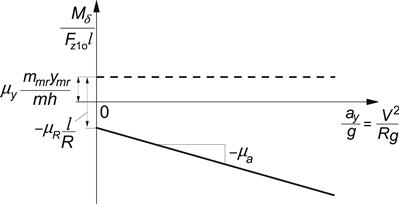
FIGURE 11.19 The non-dimensional steer torque due to path curvature 1/R and c.g. lateral offset y_mr and the variation with lateral acceleration a_y or speed V.

Numerical Results

For the baseline configuration, and the various conditions examined in Table 11.4, the values for the three steer torque coefficients have been listed in Table 11.5.

TABLE 11.5 Steer Torque Coefficients; Eqn (11.152)

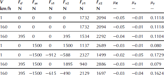
Figure 11.20 depicts the variation of the steer moment with the speed squared computed according to the approximate analytical Eqn (11.150) (dotted line) and with the exact Eqns (11.85–11.94) (including β but with φ_r = 0) together with contributing components. These components correspond with the terms of expression (11.147) and with the relevant terms of Eqn (11.89). In the contribution from the front wheel aligning torque (11.59) we distinguish the part directly attributed to F_x₁ and the remaining part indicated with The component indicated in the diagram by: F_x₁ contains the former part plus the term with F_x₁ already appearing in the β coefficient in Eqn (11.89). In both cases examined (without and with braking) the approximate total moment closely follows the course of the exact solution. The difference is largely due to the fact that in the approximate theory the twist angle has been neglected.

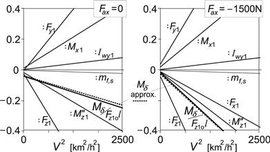
FIGURE 11.20 The non-dimensional steer torque (M_δ)/(F_z10l) and its components (cf. Eqn (11.147)) per unit non-dimensional path curvature l/R. Component denotes the aligning torque, Eqn (11.59), with F_x term deleted.

In all cases, the initial torque (V → 0) at cornering is negative (μ_R < 0), which means that when turning to the right an anti-clockwise steer torque is required. This appears to be mainly due to the direct action of the front normal load the axial component of which (F_z₁ γ₁) forms with the arm t_c a moment about the steering axis. Also the tire aligning torque with the negative slip angle of the front wheel (Figure 11.17) helps to make the steer torque negative. In the braking case, the front wheel brake force considerably increases the negative steer torque. The weights of the steerable front and subframes have an almost negligible effect, while the gyroscopic action and the front wheel side force have a tendency to make the steer torque positive.

Finally, Figure 11.21 gives the moment response to lateral offset of the center of mass of the combined rider and mainframe. The approximation is less good than we have seen so far. The deviation is largely due to the omission of the twist compliance. Because of the small side forces in this straight ahead motion we see only a very small direct effect of F_y₁. At braking, the tire torques become larger in magnitude due to the increased front slip angle and steer angle (camber), cf. Figure 11.18.

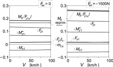
FIGURE 11.21 The non-dimensional steer torque (M_δ)/(F_z10l) and its components (cf. Eqn (11.147)) per m lateral offset of the center of gravity y_mr.

As an illustration, we consider again the case that when the motorcycle runs in a curve with a radius of 200 times the wheel base, l/R = 0.005, R = 300 m, at V= 160 km/h (= 44.4 m/s), the lateral acceleration becomes a_y = V²/R = 6.58 m/s² = 0.67 g. The vehicle is being braked and the last row of Table 11.5 applies. As a consequence, the non-dimensional torque becomes: M_δ/(F_z_1o l) =μ_R l/R + μ_a a_y/g = –0.029 × 0.005 – 0.0363 × 0.67 = –0.0245 or in dimensional form: M_δ = –0.0245 × 1732 × 1.5= –63.7 Nm. At 50 km/h we would obtain: M_δ/(F_z_1o l) = –0.0245 × 0.005 − 0.0451 × 0.0655 = –0.63 × 0.005 = −0.0031 and M_δ = –8.05 Nm. The value –0.63 corresponds to the value found in Figure 11.20 at V = 50 km/h.

For a c.g. offset of 1 cm one would find a steer torque at straight ahead running at 160 km/h: M_δ/(F_z_1o l) = μ_ym_mry_mr/mh = 0.1624 × 350 × 0.01/(390 × 0.59) = 0.0025 and M_δ = 0.0025 × 1732 × 1.5 = 6.5 Nm. The value 100 × 0.0025 = 0.25 may be predicted from Figure 11.21, where y_mr = 1 m, at 160 km/h.

11.5.2 Non-Linear Analysis of Steady-State Cornering

In this section the so-called handling diagram will be established for the motor cycle. In that diagram the variation of the (ground) steer angle can be found as a function of the lateral acceleration for a given speed of travel or for a selected value of path curvature. As additional information, the variation of the associated steer torque will be given. The diagram is similar to the handling diagrams established for the motor car in Chapter 1. The relatively large roll angle calls for special attention to assess the equilibrium condition for the front and for the rear tire.

A Simple Approximation

To introduce the problem we will again first neglect all the tire moments and the gyroscopic couples as well as the air drag. We then have the equilibrium conditions stated before:

(11.154)

while the roll angle and the front and rear camber angles become, with δ neglected with respect to the large φ:

(11.155)

and

(11.156)

(11.157)

Consequently, for a given roll angle φ we know the lateral acceleration, both side forces and the camber angles. From the non-linear tire side force characteristic that holds for the camber angle at hand and the vertical load (here equal to the static load) it must now be possible to assess the slip angle that produces, together with the camber angle, the desired side force. When we do this for both the front and rear wheels the difference in slip angles can be found and the handling curve can be drawn. At a given path curvature the ground steer angle is then easily found by using the approximate relationship:

(11.158)

Figure 11.22 shows the normalized side force characteristics according to the baseline configuration together with the equilibrium curves where the camber angle equals the roll angle belonging to the side force. In Figure 11.23 the resulting handling curve with speed lines forming the handling diagram has been presented. The speed lines indicate the relationship between lateral acceleration and path curvature for given values of speed:

(11.159)

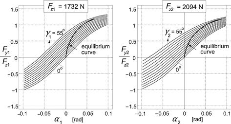
FIGURE 11.22 Tire side force diagrams at a series of camber angles γ. Simplified situation where wheel loads remain unchanged (no air drag) and tire moments and gyroscopic couples are left out of consideration. Equilibrium curves have been shown where the tire side force agrees with the roll angle (≈γ_1,2).

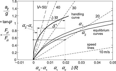
FIGURE 11.23 The handling diagram for the simplified case where tire moments and gyroscopic couples are deleted and air drag is disregarded. The normalized side force versus slip angle curves (in this simplified case equal to the equilibrium curves) have been depicted as well.

In the figure, the equilibrium curves of Figure 11.22 have been reproduced. By horizontal subtraction of these curves, the handling curve is obtained. The horizontal distance between selected speed line and the handling curve equals the ground steer angle. The slope of the handling curve with respect to the vertical axis at zero lateral acceleration corresponds to the understeer coefficient in the linear theory at constant l/R. By using Eqn (11.10) with twist angle neglected and steer angle assumed small with respect to the roll angle we find the actual steer angle:

(11.160)

The theory given above turns out to be too crude to give a reasonably accurate result. To improve the analysis, the tire moments and the gyroscopic couples should be accounted for. We may also include the effect of air drag and braking or driving forces.

To set up the equations for the steady-state cornering situation, we need to consider the conditions for equilibrium in the directions of the x, y, and z axes and about these three axes and for the steer torque: about the steering axis. We will do this for the general case with air drag introduced and with braking or driving forces acting on the front and rear wheels and possibly with a given sideways shift of the center of gravity. The twist angle β is neglected and the lean angle φ_r is disregarded since, at steady-state turning, its effect is similar to that of the c.g. lateral offset. The steer angle δ is considered small with respect to the roll angle. Also the wheel slip angles are assumed to be relatively small (smaller than ca. 10 degrees).

Equilibrium Conditions for the Complex Configuration

The condition of equilibrium in the longitudinal direction can be met by making the driving force equal to the air drag force. This means that F_x,_acc = 0 or F_x₂ = F_d. When a different driving force or when braking forces are applied, equilibrium can only be assured (a_x = 0) when the vehicle runs on an upward or downward slope. If this is not the case, we may speak of a quasi-equilibrium situation in the longitudinal direction. We have the equation (where the small longitudinal component of the side force F_y1δ′ has been neglected):

(11.161)

In the lateral direction equilibrium occurs if

(11.162)

and in the vertical direction if

(11.163)

About the x axis we have the condition:

(11.164)

about the y axis:

(11.165)

and about the z axis:

(11.166)

The wheel normal loads F_z_1,2 are found from the Eqns (11.163) and (11.165). The longitudinal tire forces F_x_1,2 are distributed according to Eqn (11.25) and as before, the acceleration force F_x,_acc is used as parameter in the handling diagrams to be developed.

With M_ya introduced for abbreviation:

(11.167)

where h_φ and h_dφ are defined by Eqn (11.5) with if relevant h replaced by h_d, we obtain the loads:

(11.168)

The two side forces are found from the Eqns (11.162) and (11.166). If we introduce for abbreviation:

(11.169)

We obtain:

(11.170)

with (from Eqn (11.10) with β = 0)

(11.171)

From Eqn (11.164) an expression for the lateral acceleration can be obtained. After using Eqn (11.60) for M_xi and the corrected effective rolling radii r_iφ:

(11.172)

and neglecting the very small contribution of δ to the moment about the x-axis we find by using the factor β_x defined as

(11.173)

for the lateral acceleration a_y = ur:

(11.174)

The Handling Diagram

For a given tanφ and y_mr the corresponding lateral acceleration a_y can be computed by using (11.174). If we disregard, as a first step, the influence of δ′ and the aligning torques M_z_1,2 in Eqns (11.170) and (11.169), we can calculate the front and rear side forces F_y_1,2 belonging to a_y. With the approximation (11.156 and 11.157) the camber angles are taken equal to the roll angle of the mainframe. It is then possible through iteration to assess the values for the slip angles α_1,2 belonging to the calculated F_ys and the known camber angles γ_1,2 with the loads obtained from (11.168 and 11.167). From the slip angles and the camber angles established, the aligning torques M_z_1,2 can be estimated for the next computation step (for a given next incremented roll angle φ) by extrapolation. Also the ground steer angle δ′ is estimated for the next step. This is done by using the Eqn (11.158) after having selected a value for the forward speed V = u. Now, a more accurate value for the side forces that belong to the equilibrium state can be found from Eqns (11.170), with (11.169). For a series of successive values of φ the values of α₁ and α₂ may be computed in this way, resulting, when plotted against a_y/g, in the equilibrium curves for the front and rear wheels (equivalent to the effective axle characteristics of Chapter 1). From the difference α₁ − α₂ the handling curve is obtained. If the air drag F_d = C_dA u² and/or a front wheel longitudinal force F_x₁ are considered, the handling curve changes with speed and the handling diagram holds only for the selected value of speed u. If air drag and front wheel braking are disregarded, a generally valid single handling curve with a series of speed lines arises as depicted in Figure 11.24. The slope at a_y = 0 is .

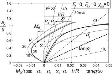
FIGURE 11.24 The handling diagram for complex model with all tire moments and gyroscopic couples included. Air drag = 0 which makes the diagram valid for all speeds V. Curves for roll angle, front and rear slip angles, and steer torque (different for each speed).

In these diagrams also the slip angles and the actual roll angle have been plotted (in abscissa direction). As an additional information, the diagram contains curve(s) for the steer torque M_δ possibly changing with speed of travel V(≈ u). How this quantity is assessed will be discussed in the subsection below.

The Steer Torque

The steer torque that is applied to the handlebar by the rider in a steady turn can be found by considering the equilibrium about the steering axis. The resulting expression is similar to the one given by Eqn (11.147) but now extended to cover large roll angles. We find with the caster length t_cφ according to Eqn (11.6):

(11.175)

with the aligning torque according to Eqn (11.59):

(11.176)

In the computations, we can use the correct expression for the camber angle γ₁ according to Eqn (11.13) with β = 0 because the steer angle δ is now available. This δ dependency causes the moment to change with path curvature and thus produces different curves for each speed value even if air drag is disregarded (Figure 11.24). The slope of the steer torque curve with respect to the vertical at a_y = 0 corresponds to μ_a F_z_1o l, cf. Table 11.5.

Results and Discussion of the Non-Linear Handling Analysis

For a number of situations the handling diagram has been established for the baseline configuration and presented in the diagrams of the Figures 11.24–11.28. The following cases have been examined:

• No air drag, no braking or driving forces, and no offset of c.g. (Figure 11.24).

• With air drag and a rear wheel driving force necessary to withstand the air drag so that the forward acceleration equals zero (F_ax = 0: neutral situation) (V = 30 m/s = 108 km/h) (Figure 11.25).

FIGURE 11.25 The handling diagram with air drag considered and zero forward acceleration (V = 108km/h).

• Braking: total deceleration force –F_ax = 1500 N (V = 108 km/h) (Figure 11.26).

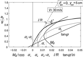
FIGURE 11.26 The handling diagram at braking (V = 108km/h).

• Hard braking: total deceleration force –F_ax = 2500 N (V = 108 km/h) (Figure 11.27).

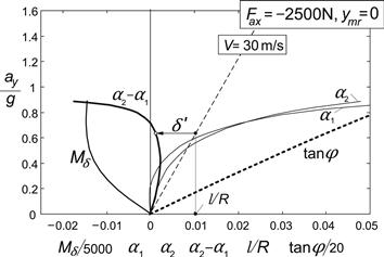
FIGURE 11.27 The handling diagram at hard braking (V = 108km/h).

• Neutral but now with lateral shift y_mr = 5 cm of the combined mass of mainframe and rider (V = 108 km/h) (Figure 11.28).

FIGURE 11.28 The handling diagram at zero forward acceleration with 5cm lateral shift of the center of gravity of combined rider and mainframe mass (V = 108km/h).

The following interesting observations may be made:

• The tire/wheel moments have a considerable influence on the resulting handling characteristic, Figure 11.24. Much more oversteer appears to occur when compared with Figure 11.23. This was already concluded from the linear theory.

• Air drag does not change handling behavior very much if the speed is not much higher than 100 km/h. The steer torque at the speed of 108 km/h appears to reach a peak, decreases, and changes in sign in the higher lateral acceleration range (Figure 11.25), where F_y₁ and M_x₁ in (11.175) become dominant.

• Braking causes the ground steer angle to become larger while the steer torque changes toward the negative direction especially at higher lateral accelerations (Figure 11.26, note the change in scale for the steer torque).

• Hard braking (Figure 11.27) tends to change the slope of the handling curve into understeer at large lateral accelerations. Also, the maximum lateral acceleration that can be reached is reduced. Larger steer angles arise in the higher a_y range of operation. Also the steer torque increases considerably in magnitude.

• The lateral c.g. shift of 5 cm gives rise to large changes in the diagram as indicated in Figure 11.28. It shows that the changes are largely due to horizontal shifts of the curves. We may compare the graph with that of Figure 11.25. Initially, at zero lateral acceleration (corresponding to Figures 11.18 and 11.21) a negative roll angle occurs while the ground steer angle δ′ and the steer torque M_δ are positive (which corresponds to and , respectively). At a certain level of lateral acceleration the steer torque reaches a minimum.

The path curvature where these minima of the steer moment or maxima of –M_δ occur constitutes the boundary of monotonous instability. At larger curvature the capsize mode becomes unstable. This is analogous to what was found for the automobile where the input is the steer angle and its maximum at a given speed of travel corresponds to the boundary of divergent (monotonous) instability (cf. Figure 1.20).

11.5.3 Modes of Vibration at Large Lateral Accelerations

The free vibrations that occur after a slight disturbance in a high lateral acceleration cornering maneuver are considerably complex in nature. Koenen (1980, 1983) studied the eigenvalues and eigenvectors of the linear homogeneous differential equations that result after linearization of the non-linear set of equations at given steady-state levels of operation. The original non-coupled in-plane and lateral out-of-plane modes of vibration appear to strongly interact with each other at larger roll angles. The weave mode occurring at straight ahead running intertwines with the bounce and pitch modes and forms three different modes of vibration in which both the in-plane and lateral degrees of freedom play a role. As a result, unstable cornering weave oscillations may arise. Similarly, the wobble mode may interact with the wheel hop mode of the front wheel, which manifests itself by a violent combined steering and vertical wheel oscillation. As an example, we present in Figure 11.29 the set of root loci in the complex plane (the eigenvalues) for both the case of straight ahead motion where we have uncoupled in-plane and out-of plane vibrations and the case where the motorcycle moves along a circular path at an average roll angle of one radian (from Koenen's work). The bounce, pitch, and hop modes appear to become almost speed independent at vanishing roll angle. In a curve, all the modes do depend on the speed of travel. In the sharp, high, lateral acceleration curving motion considered, the cornering weave root loci appear to be shifted completely to the right-hand side of the imaginary axis. The wobble mode is destabilized as well. The higher frequency twist mode (flexible frame torsion mode) keeps an individual course.

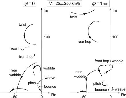
FIGURE 11.29 Eigenvalues of Koenen's motorcycle model at straight ahead running (φ = 0) and at a roll angle of one radian. The speed varies from 25 to 250km/h.

11.6 The Magic Formula Tire Model

For single track vehicles that may corner at possibly very large roll angles, a modified set of equations has been developed. To properly cover large camber angles De Vries and Pacejka (1998a) have adapted the original Magic Formulae. Since the equations listed in Chapter 4 have been revised and made more versatile and suitable to cover large camber angles, the listing of the special modified model equations has not been repeated in this new edition of the book. We may refer to the 2nd edition of this book and to the above reference for details of this special MC-MF Tire model.

The MC-MF formulae contain special features, parts of which have been incorporated in the revised set of equations presented in Section 4.3.2. Here by, these equations became suited to be employed for motorcycle tires as well.

As an example, the characteristics of a motorcycle tire, as tested by TNO with camber angle up to 45°, have been collected in the diagrams of Figure 4.33 and 4.34 in Chapter 4, similar to the presentation of the car and the truck tire characteristics.

..................Content has been hidden....................

You can't read the all page of ebook, please click here login for view all page.

Table of Contents for Chapter 11. Motorcycle Dynamics

Create new playlist

Sign In

Sign Up

Chapter 11

Motorcycle Dynamics

Chapter Outline

11.1 Introduction

11.2 Model Description

11.2.1 Geometry and Inertia

11.2.2 The Steer, Camber, and Slip Angles

11.2.3 Air Drag, Driving or Braking, and Fore-and-Aft Load Transfer

11.2.4 Tire Force and Moment Response

Linear Model

Non-Linear Model

11.3 Linear Equations of Motion

11.3.1 The Kinetic Energy

11.3.2 The Potential Energy and the Dissipation Function

11.3.3 The Virtual Work

11.3.4 Complete Set of Linear Differential Equations

11.4 Stability Analysis and Step Responses

11.4.1 Free Uncontrolled Motion

11.4.2 Step Responses of Controlled Motion

11.5 Analysis of Steady-State Cornering

11.5.1 Linear Steady-State Theory

Wheel Moments and Air Drag Neglected

Tire Overturning and Gyroscopic Couples Included

Tire Yaw Moments Included

Driving and Braking Forces Included

Numerical Results

The Steer Torque

Numerical Results

11.5.2 Non-Linear Analysis of Steady-State Cornering

A Simple Approximation

Equilibrium Conditions for the Complex Configuration

The Handling Diagram

The Steer Torque

Results and Discussion of the Non-Linear Handling Analysis

11.5.3 Modes of Vibration at Large Lateral Accelerations

11.6 The Magic Formula Tire Model

Table of Contents for
Chapter 11. Motorcycle Dynamics