
Chapter 3
Theory of Steady-State Slip Force and Moment Generation
Chapter Outline
3.2.3. Interaction between Lateral and Longitudinal Slip (Combined Slip)
3.3. The Tread Simulation Model
3.4. Application: Vehicle Stability at Braking up to Wheel Lock
3.1 Introduction
This chapter is devoted to the analysis of the properties of a relatively simple theoretical tire model belonging to the third category of Figure 2.11. The mathematical modeling of the physical model shown in Figure 2.13 has been a challenge to various investigators. Four fundamental factors play a role: frictional properties in the road-tire interface, distribution of the normal contact pressure, compliance of the tread rubber, and compliance of the belt/carcass.
Models of the carcass with belt and side walls with encapsulated pressurized air that are commonly encountered in the tire modeling literature are based either on an elastic beam or on a stretched string both suspended on an elastic foundation with respect to the wheel rim. The representation of the belt by a beam instead of by a stretched string is more difficult because of the fact that the differential equation that governs the lateral deflection of the belt under the action of a lateral force becomes of the fourth instead of the second order. For the study of steady-state tire behavior, most authors approximate the more or less exact expressions for the lateral deflection of the beam or string.
As an extension to the original ‘brush’ model of Fromm and of Julien (cf. Hadekel (1952) for references) who did not consider carcass compliance, Fiala (1954) and Freudenstein (1961) developed theories in which the carcass deflection is approximated by a symmetric parabola. Böhm (1963) and Borgmann (1963), the latter without the introduction of tread elements, used asymmetric approximate shapes determined by both the lateral force and the aligning torque. Pacejka (1966, 1981) established the steady-state side-slip characteristics for a stretched-string-tire model without and with the inclusion of tread elements attached to the string. The lateral stiffness distribution as measured on a slowly rolling tire in terms of influence or Green’s functions (cf. Savkoor 1970) may be employed in a model for the side-slipping tire possibly in connection with the tread-element-following method that was briefly discussed in the preceding section (cf. Pacejka 1972, 1974) and will be demonstrated later on in Section 3.3 of the present chapter.
Frank (1965a) has carried out a thorough comparative investigation of the various one-dimensional models. He employed a general fourth-order differential equation with which tire models can be examined that feature a stretched string, a beam, or a stretched beam provided with elastic tread elements. Frank obtained a solution of the steady-state slip problem with the aid of a special analog computer circuit. A correlation with Fourier components of the measured deformation of real tires reveals that the stretched string-type model seems to be more suitable for the simulation of a bias ply tire, whereas the beam model is probably more appropriate for representing the radial ply tire.
Figure 3.1 (from Frank 1965b) presents the calculated characteristics of several types of carcass models provided with tread elements. The curves represent: a. stretched string model, b. beam model, c. approximation based on Fiala’s model (symmetric parabolic carcass deflection), d. model of Fromm (brush model with rigid carcass). The tread element stiffness is the same for each model. The parameters in the cases a, b, and c have been chosen in such a way as to give a best fit to experimental data for the peak side force and the cornering force at small slip angles (that is, same cornering stiffness). It appears then that model c shows close correspondence with curve a for the side force. Curves d show the result when the carcass elasticity is neglected and only the flexibility of the tread elements is taken into account. When the tread element stiffness of model d is adapted (i.e., lowered) in such a way that the cornering stiffness becomes equal to that of the other three models, no difference between the side force characteristics according to Fromm’s and Fiala’s models appears to occur. Due to approximations introduced by Fiala, the coefficients in the expression for the side force versus slip angle (if parabolic pressure distribution is adopted) become equal to those obtained directly by Fromm.
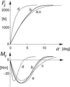
FIGURE 3.1 Comparison of calculated characteristics for four different tire models with tread elements and nonsymmetrical pressure distribution at a given wheel vertical load (a: string, b: beam, c: Fiala, d: brush i.e., with rigid carcass) (from Frank 1965a,b).
In the calculations for Figure 3.1, Frank employed a constant coefficient of friction μ and a slightly asymmetric vertical pressure distribution qz(x), found from measurements. The positive aligning torque obtained at larger values of the slip angle α arises as a result of this asymmetry. The phenomenon that in practice the aligning torque indeed varies in this way is due to a combination of several effects. The main cause is probably connected with the asymmetric pressure distribution of the rolling tire (due to hysteresis of the tire compound) resulting in a small forward shift of the point of application of the normal load (giving rise to rolling resistance) and, consequently, at full sliding also of the resulting side force. Another important factor causing the moment to become positive is the fact that the coefficient of friction is not a constant but tends to decrease with sliding velocity. As may be derived from e.g., Eqn (2.59), the sliding velocity attains its largest values in the rear portion of the contact area where the slope ![]() becomes largest. Consequently, we expect to have larger side forces acting in the front half of the contact area at full sliding conditions than in the rear half. The rolling resistance force that due to the lateral distortion acts slightly beside the wheel plane may also contribute to the sign change of Mz. A μ that decreases with the sliding velocity (not considered by Frank) causes the creation of a peak in the Fy(α) curves and a further slight decay. This has often been observed to occur in practice, especially on wet and icy roads. In the longitudinal force characteristic the peak is usually more pronounced.
becomes largest. Consequently, we expect to have larger side forces acting in the front half of the contact area at full sliding conditions than in the rear half. The rolling resistance force that due to the lateral distortion acts slightly beside the wheel plane may also contribute to the sign change of Mz. A μ that decreases with the sliding velocity (not considered by Frank) causes the creation of a peak in the Fy(α) curves and a further slight decay. This has often been observed to occur in practice, especially on wet and icy roads. In the longitudinal force characteristic the peak is usually more pronounced.
The influence of different but symmetric shapes for the vertical force distribution along the x-axis has been theoretically investigated by Borgmann (1963). He finds that, especially for tires exhibiting a relatively large carcass compliance, the influence of the pressure distribution is of importance. Nonsymmetric more general distributions were studied by Guo (1994). Many authors adopt, for the purpose of mathematical simplicity, the parabolic distribution (Fiala 1954, Freudenstein 1961, Bergman 1965, Pacejka 1958, Sakai (also n-th degree parabola, 1989), Dugoff et al. 1970 (uniform, rectangular distribution) and Bernard et al. 1977 (trapezium shape)). Models of Fiala and Freudenstein feature a flexible carcass while the remaining authors have restricted themselves to a rigid carcass or a uniformly deflected belt. That, however, enabled them to include the description of the more difficult case of combined slip. The introduction of a nonconstant friction coefficient has been treated by others: Böhm (1963), Borgmann (1963), Dugoff et al. (1970), Sakai (1981), and Bernard et al. (1977).
Figure 3.1 shows that, when the model parameters are chosen properly, the choice of the type of carcass model (beam, string, or rigid) has only a limited effect. Qualitatively, the resulting curves are identical. The rigid carcass model with elastic tread elements is often referred to as the brush tire model. Because of its simplicity and qualitative correspondence with experimental tire behavior, we will give a full treatment of its properties, mainly to provide understanding of steady-state tire slipping properties which may also be helpful in the development of more complex models. A uniform carcass deflection will be considered to improve the aligning torque representation at combined slip.
In Section 3.3, we deal with the effect of nonuniform carcass deflection, nonconstant friction coefficient, and the inclusion of camber and turning (path curvature) combined with side slip and braking/driving. For this purpose, the tread simulation model will be employed.
3.2 Tire Brush Model
The brush model consists of a row of elastic bristles that touches the road plane and can deflect in a direction parallel to the road surface. These bristles may be called tread elements. Their compliance represents the elasticity of the combination of carcass, belt, and actual tread elements of the real tire. As the tire rolls, the first element that enters the contact zone is assumed to stand perpendicularly with respect to the road surface. When the tire rolls freely (that is without the action of a driving or braking torque) and without side slip, camber, or turning, the wheel moves along a straight line parallel to the road and in the direction of the wheel plane. In that situation, the tread elements remain vertical and move from the leading edge to the trailing edge without developing a horizontal deflection and consequently without generating a fore-and-aft or side force. A possible presence of rolling resistance is disregarded. When the wheel speed vector V shows an angle with respect to the wheel plane, side slip occurs. When the wheel velocity of revolution Ω multiplied with the effective rolling radius re is not equal to the forward component of the wheel speed Vx = Vcos α, we have fore-and-aft slip. Under these conditions, depicted in Figure 3.2, horizontal deflections are developed and corresponding forces and moment arise. The tread elements move from the leading edge (on the right-hand side of the pictures) to the trailing edge. The tip of the element will, as long as the available friction allows, adhere to the ground (that is, it will not slide over the road surface). Simultaneously, the base point of the element remains in the wheel plane and moves backward with the linear speed of rolling Vr (that is equal to reΩ) with respect to wheel axis or better: with respect to the contact center C. With respect to the road, the base point of the element moves with a velocity that is designated as the slip speed Vs of the wheel.
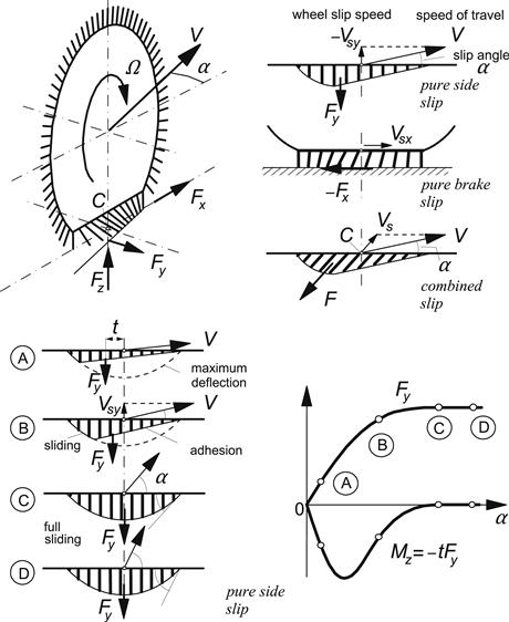
FIGURE 3.2 The brush tire model. Top left: view of driven and side-slipping tire. Top right: the tire at different slip conditions. Bottom left: the tire at pure side slip, from small to large slip angle. Bottom right: the resulting side force and aligning torque characteristics.
In the lower part of the figure, the model is shown at pure side slip. The slip changes from very small to relatively large. We observe that the deflection increases while the element moves further through the contact patch. The deflection rate is equal to the supposedly constant slip speed. The resulting deflection varies linearly with the distance to the leading edge and the tips form a straight contact line that lies in a direction parallel to the wheel speed vector V. The figure also shows the maximum possible deflection that can be reached by the element depending on its position in the contact region. This maximum is governed by the (constant) coefficient of friction μ, the vertical force distribution qz, and the stiffness of the element cpy. The pressure distribution and consequently also the maximum deflection vmax have been assumed to vary according to a parabola. As soon as the straight contact line intersects the parabola, sliding will start. The remaining part of the contact line will coincide with the parabola for the maximum possible deflection. At increasing slip angle, the side force that is generated will increase. The distance of its line of action behind the contact center is termed the pneumatic trail t. The aligning torque arises through the nonsymmetric shape of the deflection distribution and will be found by multiplying the side force with the pneumatic trail. As the slip increases, the deformation shape becomes more symmetric and, as a result, the trail gets smaller. This is because the point of intersection moves forward, thereby increasing the sliding range and decreasing the range of adhesion. This continues until the wheel speed vector runs parallel to the tangent to the parabola at the foremost point. Then, the point of intersection has reached the leading edge and full sliding starts to occur. The shape has now become fully symmetric. The side force attains its maximum and acts in the middle so that the moment vanishes. That situation remains unchanged when the slip angle increases further. The resulting characteristics for the side force and the aligning torque have been depicted in the same figure. In the part to follow next, the mathematical expressions for these relationships will be derived, first for the case of pure side slip.
3.2.1 Pure Side Slip
The brush model moving at a constant slip angle has been depicted in greater detail in Figure 3.3. It shows a contact line which is straight and parallel to the velocity vector V in the adhesion region and curved in the sliding region where the available frictional force becomes lower than the force which would be required for the tips of the tread elements to follow the straight line further. In the adhesion region the linear variation of the deformation is in accordance with the general equation (2.65) (where tan α has been assumed small and replaced by α) with at steady state ![]() . For this simple model, the deformation of the tread element at the leading edge vanishes. Consequently, the lateral deformation in the adhesion region reads
. For this simple model, the deformation of the tread element at the leading edge vanishes. Consequently, the lateral deformation in the adhesion region reads
![]() (3.1)
(3.1)
where a denotes half the contact length.
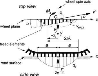
FIGURE 3.3 Brush model moving at pure side slip shown in top and side view.
In the case of vanishing sliding, that will occur for ![]() or for
or for ![]() , expression (3.1) is valid for the entire region of contact. With the lateral stiffness cpy of the tread elements per unit length of the assumedly rectangular contact area, the following integrals and expressions for the cornering force Fy and the aligning torque Mz hold:
, expression (3.1) is valid for the entire region of contact. With the lateral stiffness cpy of the tread elements per unit length of the assumedly rectangular contact area, the following integrals and expressions for the cornering force Fy and the aligning torque Mz hold:
 (3.2)
(3.2)
Consequently, the cornering stiffness and the aligning stiffness become, respectively,
 (3.3)
(3.3)
Next, we will consider the case of finite μ and a pressure distribution which gradually drops to zero at both edges. For the purpose of simplicity, we assume a parabolic distribution of the vertical force per unit length as expressed by
![]() (3.4)
(3.4)
where Fz represents the vertical wheel load. Hence, the largest possible side force distribution becomes
![]() (3.5)
(3.5)
In Figure 3.3 the maximum possible lateral deformation vmax = qy,max/cpy has been indicated. For the sake of abbreviation, the following composite tire model parameter is introduced:
![]() (3.6)
(3.6)
The distance from the leading edge to the point, where the transition from the adhesion to the sliding region occurs, is written as 2aλ and is determined by the factor λ. The value of this nondimensional quantity is found by realizing that at this point, where x = xt, the deflection in the adhesion range becomes equal to that of the sliding range. Hence, with Eqns (3.1, 3.5, 3.6) the following equality holds:
![]() (3.7)
(3.7)
and thus for λ = (a − xt)/2a we obtain the relationship with the slip angle α:
![]() (3.8)
(3.8)
From this equation, the angle αsl, where total sliding starts (λ = 0), can be calculated:
![]() (3.9)
(3.9)
As the distribution of the deflections of the elements has now been established, the total force Fy and the moment Mz can be assessed by integration over the contact length (like in Eqn (3.2) but now separate for the sliding range −a < x < xt and the adhesion range xt < x < a). For convenience, we introduce the notation for the slip:
![]() (3.10)
(3.10)
The resulting formula for the force reads:
if |α| ≤ αsl
![]() (3.11)
(3.11)
and, if |α| ≥ αsl (but < ½π),
![]() (3.11a)
(3.11a)
and for the moment:
if |α| ≤ αsl
![]() (3.12)
(3.12)
with peak value 27μFz/256 at σy = 1/(4θy);
if |α| ≥ αsl (but < ½π):
![]() (3.12a)
(3.12a)
The pneumatic trail t, which indicates the distance behind the contact center C where the resultant side force Fy is acting, becomes
if |α| ≤ αsl
![]() (3.13)
(3.13)
and if |α| ≥ αsl (but < ½π)
![]() (3.13a)
(3.13a)
These relationships have been shown graphically in Figure 3.4. At vanishing, slip angle expression (3.13) reduces to
![]() (3.14)
(3.14)
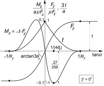
FIGURE 3.4 Characteristics of the simple brush model: side force, aligning torque, and pneumatic trail vs slip angle.
This value is smaller than normally encountered in practice. The introduction of an elastic carcass will improve this quantitative aspect. Then, the more realistic value of t ≈ 0.5a may be achieved (cf. Pacejka 1966 for a stretched string model to represent the elastic carcass and Section 3.3 for a more generally applicable way of approach to account for the carcass compliance). Another point in which the simple model deviates considerably from experimental results concerns the effect of changing the vertical wheel load Fz. With the assumption that the contact length 2a changes quadratically with radial tire deflection ρ and that Fz depends linearly on ρ, so that a2∼Fz, it can be easily shown that for the brush model Fy and Mz vary proportionally with Fz and Fz3/2, respectively. Experiments, however, show that Fy varies less than linearly with Fz. In most cases, the Fy vs Fz characteristic, obtained at a small value of the slip angle, even shows a maximum after which the cornering force drops with increasing wheel load. Obviously, the same holds for the cornering stiffness CFα (cf. Figure 1.3). Also in this respect the introduction of an elastic carcass (in particular when its lateral stiffness decreases with increasing normal load) improves the agreement with experiments. When considering a deflected cross section of a tire with side walls modeled as membranes under tension encapsulating pressurized air, such a decrease in lateral stiffness can be found to occur in theory (cf. Pacejka 1981, pp. 729 and 730).
An interesting diagram is the so-called Gough plot, in which Fy is plotted vs Mz for a series of constant values of Fz (or possibly of μ at constant Fz) and of α respectively. This produces two sets of curves shown in Figures 3.5 and 3.6. In the first figure, the characteristics for the brush model have been presented. The left-hand diagram shows that when made nondimensional, a single curve results. The second figure presents the measured curves for a truck tire and in addition a diagram according to the brush model. The model has been adapted to include the nonlinear relationship of the cornering stiffness vs vertical load by making the tread element stiffness decrease linearly with vertical load. As can be seen from the left-hand plot (at large values of α where saturation of Fy occurs), the truck tire also exhibits a decay in friction coefficient with increasing vertical load (not included in the model calculations), cf. also Figure 1.3. Further, as expected, the actual tire generates an aligning torque larger than that according to the model.
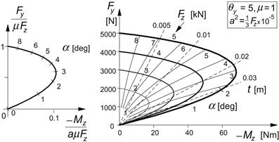
FIGURE 3.5 The so-called Gough plot for the brush model, nondimensional, and with dimension using an assumed load vs contact length relationship.
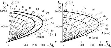
FIGURE 3.6 Left: Gough plot of truck tire 9.00–20, measured on a dry road surface (Freudenstein 1961). Right: brush model with tread element stiffness cp decaying linearly with Fz.
3.2.2 Pure Longitudinal Slip
For the brush-type tire model with tread elements flexible in longitudinal direction, the theory for longitudinal (braking or driving) force generation develops along similar lines as those set out in Section 3.2.1 where the side force and aligning torque response to slip angle have been derived. To simplify the discussion, we restrict ourselves here to non-negative values of the forward speed Vx and of the speed of revolution Ω.
In Figure 3.7 a side view of the brush model has been shown. As indicated before, the so-called slip point S is introduced. This is an imaginary point attached to the wheel rim and is located, at the instant considered, a distance equal to the effective rolling radius re (defined at free rolling) below the wheel center. At free rolling, by definition, the slip point S has a velocity equal to zero. Then, it forms the instantaneous center of rotation of the wheel rim. We may think of a slip circle with radius re that in the case of free rolling rolls perfectly, that is, without sliding, over an imaginary road surface that touches the slip circle in point S. When the wheel is being braked, point S moves forward with the longitudinal slip velocity Vsx. When driven, the slip point moves backward with consequently a negative slip speed. In the model, a point S′ is defined that is attached to the base line at its center (that is, at the base point of the tread element below the wheel center, cf. Figure 3.7). By definition, the velocity of this point is the same as that of point S. That means that S′ also moves with the same slip speed Vsx. It is assumed that the tread elements attached at their base points to the circumferentially rigid carcass enter the contact area in vertical position. At free rolling with slip speed Vsx (of both points S and S′) equal to zero, the orientation of the elements remains vertical while moving from front to rear through the contact zone. Consequently, no longitudinal force is being transmitted and we have a wheel speed of revolution:
![]() (3.15)
(3.15)
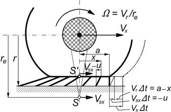
FIGURE 3.7 Side view of the brush tire model at braking (no sliding considered).
Here it is assumed that the longitudinal component of the speed of propagation of the contact center C is equal to the longitudinal component of the speed of the wheel center (Vcx = Vx). As has been seen in the previous chapter, this will occur on a flat road surface at vanishing ![]() . When Ω differs from its value at free rolling Ωo, the wheel is being braked or driven and the longitudinal slip speed Vsx becomes
. When Ω differs from its value at free rolling Ωo, the wheel is being braked or driven and the longitudinal slip speed Vsx becomes
![]() (3.16)
(3.16)
In the model, the base points of all the tread elements move with the same speed Vsx. A base point progresses backward through the contact zone with a speed Vr called the linear speed of rolling. Apparently, we have
![]() (3.17)
(3.17)
An element the tip of which adheres to the ground and the base point is moved toward the rear over a distance a − x from the leading edge (for which a time span Δt = (a − x)/Vr is needed) has developed a deflection in longitudinal direction:
![]() (3.18)
(3.18)
The same expression may be obtained by integration of the fundamental equation (2.55) and noting that Vgx = ωz = ∂u/∂t = θ’s = 0 and finally using the boundary condition u = 0 at x = a.
We may write the longitudinal deflection u in terms of the ‘practical’ longitudinal slip κ = −Vsx/Vx:
![]() (3.19)
(3.19)
In terms of the alternative definition of longitudinal slip, the ‘theoretical’ slip is to be used in the subsequent section and defined as
![]() (3.20)
(3.20)
(note, we restrict ourselves to non-negative speeds of rolling: Vr ≥ 0 and κ ≥ −1). We obtain
![]() (3.21)
(3.21)
In Section 3.2.l, we found with Eqns (3.1) and (3.10) for the lateral deflection at pure side slip (σy = tan α):
![]() (3.22)
(3.22)
Comparison of the Eqns (3.21) and (3.22) shows that the longitudinal deformations u will be equal in magnitude to the lateral deformations v if σy = tan α equals σx = κ/(1 + κ). For equal tread element stiffnesses (cpx = cpy) and friction coefficients (μx = μy) in lateral and longitudinal directions, the slip force characteristics in both directions are identical when tan α and κ/(1 + κ) are used as abscissa (cf. Figure 3.8). Also, Eqn (3.11) holds for the longitudinal force Fx if the subscripts y are replaced by x and tan α by κ.
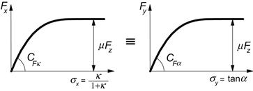
FIGURE 3.8 Equality of the two pure slip characteristics for an isotropic tire model if plotted against the theoretical slip.
Obviously, total sliding will start at σx = κ/(1 + κ) = ±1/θx or in terms of the practical slip at
![]() (3.23)
(3.23)
with
![]() (3.24)
(3.24)
Linearization for small values of slip κ yields a deflection at coordinate x:
![]() (3.25)
(3.25)
![]() (3.26)
(3.26)
with cpx the longitudinal tread element stiffness per unit length. This relation contains the longitudinal slip stiffness:
![]() (3.27)
(3.27)
For equal longitudinal and lateral stiffnesses (cpx = cpy), we obtain equal slip stiffnesses CFκ = CFα. In reality, however, appreciable differences between the measured values of CFκ and CFα may occur (say CFκ about 50% larger than CFα) which is due to the lateral (torsional) compliance of the carcass of the actual tire. Still, it is expected that qualitative similarity of both pure slip characteristics remains.
3.2.3 Interaction between Lateral and Longitudinal Slip (Combined Slip)
For the analysis of the influence of longitudinal slip (or longitudinal force) on the lateral force and moment generation properties, we shall, for the sake of mathematical simplicity, restrict ourselves to the case of equal longitudinal and lateral stiffnesses of the tread elements (isotropic model), i.e.,
![]() (3.28)
(3.28)
and equal and constant friction coefficients
![]() (3.29)
(3.29)
Again a parabolic pressure distribution is considered.
Figure 3.9 depicts the deformations which arise when the tire model which runs at a given slip angle α is driven or braked. Due to the equal stiffness in all horizontal directions and the isotropic friction properties, the deflections are directed opposite to the slip speed vector Vs, also in the sliding region. In this latter region, the tips of the elements slide over the road with sliding speed Vg directed opposite to the local friction force q (per unit contact length). The whole deformation history of a tread element, while running through the contact area, is a one-dimensional process along the direction of Vs.
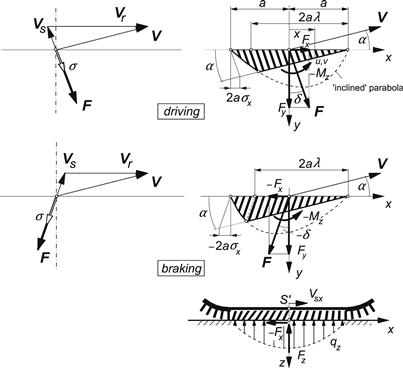
FIGURE 3.9 Vector diagram and deformation of the brush model running at a given slip angle for the cases of driving and braking.
The velocity of progression of a base point through the contact length is the rolling speed Vr (again assumed non-negative). The deflection rate of an element in the adhesion region is equal to the slip speed Vs. The time which elapses from the point of entrance to the point at a distance x in front of the contact center equals
![]() (3.30)
(3.30)
In this position, the deflection of an element that is still in adhesion becomes in vectorial form
![]() (3.31)
(3.31)
It seems natural at this stage to introduce the alternative (theoretical) slip quantity again, but now in vectorial form:
![]() (3.32)
(3.32)
with the linear speed of rolling
![]() (3.33)
(3.33)
The relations of these theoretical slip quantities with the practical slip quantities κ (= −Vsx /Vx) and tan α (= −Vsy /Vx) are
![]() (3.34)
(3.34)
The deflection of an element in the adhesion region now reads
![]() (3.35)
(3.35)
from which it is apparent that longitudinal and lateral deflections are governed by σx and σy respectively and independent of each other. This would not be the case if expressed in terms of the practical slip quantities κ and α!
The local horizontal contact force acting on the tips of the elements (per unit contact length) reads
![]() (3.36)
(3.36)
As soon as
![]() (3.37)
(3.37)
the sliding region is entered. Then the friction force vector becomes
![]() (3.38)
(3.38)
where
![]() (3.39)
(3.39)
and
![]() (3.40)
(3.40)
Similarly, the magnitude of the deflection of an element becomes
![]() (3.41)
(3.41)
The point of transition from adhesion to sliding region is obtained from the condition
![]() (3.42)
(3.42)
or
![]() (3.43)
(3.43)
which yields
![]() (3.44)
(3.44)
or, in similar terms as Eqn (3.8),
![]() (3.45)
(3.45)
where analogous to expressions (3.6) and (3.24) for the isotropic model parameter θ reads
![]() (3.46)
(3.46)
From Eqn (3.45), the slip σsl at which total sliding starts can be calculated. We get, analogous to (3.9),
![]() (3.47)
(3.47)
The magnitude of the total force F = |F| now easily follows in accordance with (3.11):
![]() (3.48)
(3.48)
and obviously follows the same course as those shown in Figure 3.8. The force vector F acts in a direction opposite to Vs or −σ. Hence,
![]() (3.49)
(3.49)
from which the components Fx and Fy may be obtained.
The moment −Mz is obtained by multiplication of Fy with the pneumatic trail t. This trail is easily found when we realize that the deflection distribution over the contact length is identical with the case of pure side slip if tan αeq = σ (cf. Figure 3.10). Consequently, formula (3.13) represents the pneumatic trail at combined slip as well if θyσy is replaced by θσ. We have, with (3.13),
![]() (3.50)
(3.50)
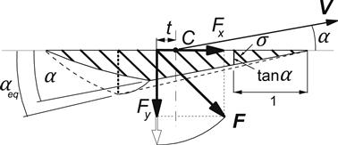
FIGURE 3.10 Equivalent side-slip angle producing the same pneumatic trail t.
In Figures 3.11 and 3.12, the dramatic reduction of the pure slip forces (the side force and the longitudinal force respectively) that occurs as a result of the simultaneous introduction of the other slip component (the longitudinal slip and the side slip respectively) has been indicated. We observe an (almost) symmetric shape of these interaction curves. The peak of the side force vs longitudinal slip curves at constant values of the slip angle appears to be slightly shifted toward the braking side. This phenomenon will be further discussed in connection with the alternative representation of the same results according to Figure 3.13. At very large longitudinal slip that is when |Vsx|/Vx → ∞, the side force approaches zero and the same occurs for the longitudinal force when the lateral slip tan α goes to infinity (α → 90°) at a given value of the longitudinal slip because obviously in that case with Vx → 0 also the longitudinal slip speed must vanish. For a locked wheel with Vsx = Vx and κ = −1, we have Fy = μFz sin α and Fx = −μFz cos α.
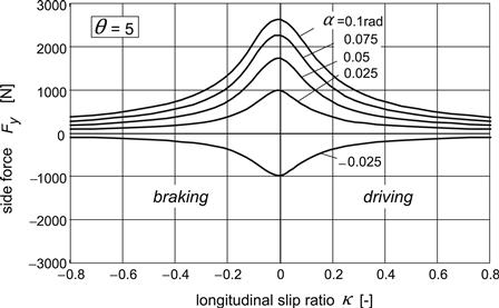
FIGURE 3.11 Reduction of side force due to the presence of longitudinal slip.
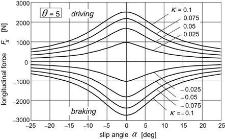
FIGURE 3.12 Reduction of longitudinal force due to the presence of side slip.
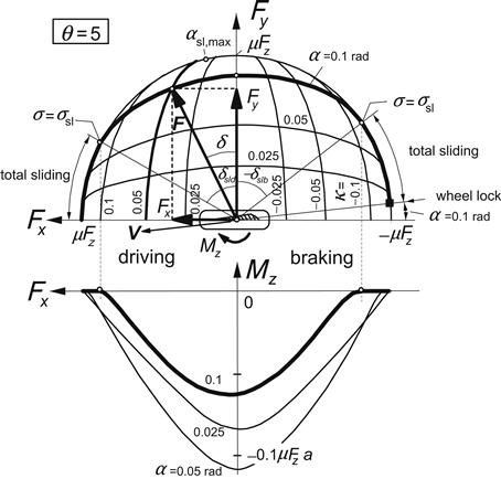
FIGURE 3.13 Cornering force and aligning torque as functions of longitudinal force at constant slip angle α or longitudinal slip κ.
In the diagram of Figure 3.13, the calculated variations of Fy and Mz with Fx have been plotted for several fixed values of α. Also, the curves for constant κ have been depicted. For clarification of the nature of the Fy − Fx diagram, the deflection of an element near the leading edge has been shown in Figure 3.14. Since the distance from the leading edge has been defined for this occasion to be equal to unity, the deflection e of the element equals the slip σ. The radius of the circle denoting maximum possible deflections is equal to σsl. The two points on the circle where the slip angle α considered the sliding boundary σsl is attained correspond to the points on the α curve of the force diagram of Figure 3.13. This also explains the slightly inclined nature of the α curves. At braking, Fy appears to be a little larger than at driving. This is at least true for the two cases of Figure 3.9, one at driving and the other at braking, showing the same slip angle and the same magnitude of the deviation angle δ of the slip velocity vector and thus of the force vector with respect to the y-axis. Then, the slip speeds Vs are equal in magnitude, but at braking the speed of rolling Vr is obviously smaller. When considering the definition of the theoretical slip σ (3.32) and the functional relationship (3.48) with the force F, it becomes clear that F must be larger for the case of braking because of the then larger magnitude of σ. Finally, the case of wheel lock is pointed at. Then, the force vector F, which in magnitude is equal to μFz, is directed opposite to the speed vector of the wheel V which then coincides with the slip speed vector Vs.
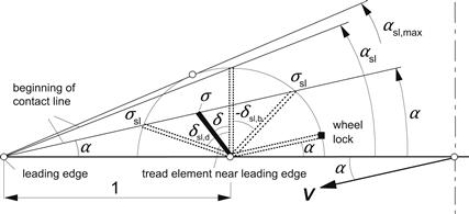
FIGURE 3.14 The situation near the leading edge. Various deflections of an element at a distance equal to 1 from the leading edge are shown corresponding with points in the upper diagram of Figure 3.13.
Experimental evidence (e.g., Figure 3.17) supports the nature of the theoretical curves for the forces as shown in Figure 3.13. Often, the shape appears to be more asymmetric than predicted by the simple brush model. This may be due to a slight increase in the contact length while braking (making the tire stiffer) and by the brake force-induced slip angle of the contact patch at side slip. This is accomplished through the torsion of the carcass induced by the moment about the vertical axis that is exerted by the braking force which has shifted its line of action due to the lateral deflection connected with the side force. The more advanced model to be developed further on in this chapter will take the latter effect into account.
The moment curves presented in the lower diagram of Figure 3.13 show a more or less symmetrical bell shape. As expected, the aligning torque becomes equal to zero when total sliding occurs (σ ≥ σsl). Later on, we will see that these computed moment characteristics may appreciably deviate from experimentally obtained curves.
At this stage, we will first apply the knowledge gained so far to the analysis of a practical situation that occurs with a wheel that is braked or driven (at constant brake pressure and throttle respectively) while its slip angle is varied.
In Figure 3.15, the force diagram is shown in combination with the corresponding velocity diagram. At a given braking force −Fx and wheel speed of travel V, the slip angle α is changed from zero to 90°. The variation of slip speed Vs and rolling speed Vr may be followed from case 1 where α = 0 to case 3 where total sliding starts and further to case 4 where Vr and thus Ω vanish and the wheel becomes locked. A further increase of α (at constant brake pedal force) as in case 5 will necessarily lead to a reduction in braking force −Fx unless the wheel is rotated in opposite direction (Ω < 0) as represented by case 5′. In the cases of driving indicated by Roman numerals, the driving force Fx can be maintained irrespective of the value of α (with |α| < 90°).
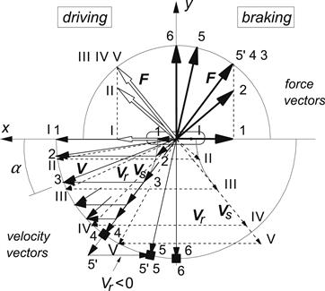
FIGURE 3.15 The Fx − Fy diagram extended with the corresponding velocity diagram. The brake (pedal) force is kept constant while the slip angle is increased. The same is done at a constant driving effort. In the case of braking, the speed of rolling Vr decreases until the wheel gets locked. In the special case 5′, the wheel is rotated backward to keep the slip speed Vs and thus the force vector F in the original direction.
The nature of the resulting Fy−α characteristics at given driving or braking effort is shown in Figure 3.16. Plotting of Fy versus sin α is advantageous because the portion where wheel lock occurs is then represented by a straight line.
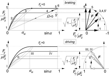
FIGURE 3.16 Tire characteristics at constant brake (pedal) force and driving force. Numerals correspond to those of Figure 3.15.
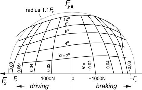
FIGURE 3.17 Fy – Fx characteristics for 6.00–13 tire measured on dry internal drum with diameter of 3.8 m (from Henker 1968).
Another important advantage of putting sin α instead of tan α along the abscissa is that (after having completed the diagram for negative values of sin α resulting in an oddly symmetric graph) the complete range of α is covered: the speed vector V may swing around over the whole range of 360°. An application in vehicle dynamics will be discussed in Section 3.4 (yaw instability at locked rear wheels).
For illustration we have shown in Figures 3.17 and 3.18 experimentally assessed characteristics. The force diagrams correspond reasonably well with the theoretical observations. The moment curves, however, deviate considerably from the theoretical predictions (compare Figure 3.18 with Figure 3.13). It appears that according to this figure, Mz changes its sign in the braking half of the diagram. This phenomenon can not be explained with the simple tire brush model that has been employed thus far.
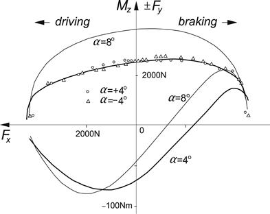
FIGURE 3.18 Combined slip side force and moment vs longitudinal force characteristics measured at two values of the slip angle for a 7.60–15 tire on a dry flat surface (from Nordeen and Cortese 1963).
The introduction of a laterally flexible carcass seems essential for properly modeling Mz that acts on a driven or braked wheel. In Figure 3.19, a possible extension of the brush model is depicted. The carcass line is assumed to remain straight and parallel to the wheel plane in the contact region. A lateral and longitudinal compliance with respect to the wheel plane is introduced. In addition, a possible initial offset of the line of action of the longitudinal force with respect to the wheel center plane is regarded. Such an offset is caused by asymmetry of the construction of the tire or by the presence of a camber angle.
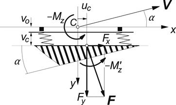
FIGURE 3.19 Extended tire brush model showing offset and deflection of carcass line (straight and parallel to wheel plane).
With this model, the moment Mz is composed of the original contribution ![]() established by the brush model and those due to the forces Fy and Fx which show lines of action shifted with respect to the contact center C over the distances uc and vo + vc, respectively. The self-aligning torque now reads
established by the brush model and those due to the forces Fy and Fx which show lines of action shifted with respect to the contact center C over the distances uc and vo + vc, respectively. The self-aligning torque now reads
![]() (3.51)
(3.51)
where the compliance coefficient c has been introduced that is defined by
![]() (3.52)
(3.52)
Here Ccx and Ccy denote the longitudinal and lateral carcass stiffnesses respectively and εx and εy the effective fractions of the actual displacements. These fractions must be considered because of concurrent lateral and longitudinal rolling of the tire lower section against the road surface under the action of a lateral and fore-and-aft force respectively which will change the normal force distribution in the contact patch and thereby reduce the actual displacements of the lines of action of both horizontal forces. The resulting calculations can be performed in a direct straightforward manner, because the slip angle of the extended model is the same as the one for the internal brush model. Later on, in Section 3.3, the effect of the introduction of a torsional and bending stiffness of the carcass and belt will be discussed. The resulting model, however, is a lot more complex and closed form solutions are no longer possible. In Section 3.3, the technique of the tread element following method will be employed in the tread simulation model to determine the response.
The combined slip response of the simple extended model of Figure 3.19 is given in Figures 3.20 and 3.21. It is observed that in Figure 3.20, the aligning torque changes its sign in the braking range. This is due to the term in Eqn (3.51) with the compliance coefficient c. The resulting qualitative shape is quite similar to the experimentally found curves of Figure 3.18. In Figure 3.21, the effect of an initial offset of vo = 5 mm has been depicted.
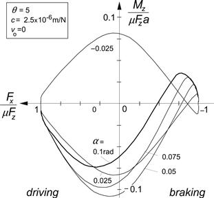
FIGURE 3.20 The influence of lateral carcass compliance on the aligning torque for a braked or driven wheel according to the extended brush model.
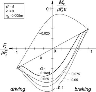
FIGURE 3.21 The influence of an initial lateral offset vo of Fx on the aligning torque for a braked or driven wheel according to the extended brush model.
Here carcass compliance has been disregarded and only the last term of (3.51) has been added. We see that a moment is generated already at zero slip angle. The curves found in Figure 3.13 for nonzero side slip are then simply added to the inclined straight line belonging to α = 0. The type of curves that result are often found experimentally. The effect of lateral compliance may then be very small or canceled out by the effect of the fore-and-aft compliance of the carcass (second term of right-hand member of (3.52)).
Exercise 3.1. Characteristics of the Brush Model
Consider the brush tire model as treated in Section 3.2. Elastic and frictional properties are the same in all horizontal directions and Eqn (3.46) holds.
For 0 ≤ α ≤ ½π, the side force characteristic is described by (according to Eqn (3.11))
![]()
1. Calculate the value of θ and tan αsl for
μFz = 2000 N
CFα = 18000 N/rad
2. Sketch the Fy(tan α) characteristic and also the Mz(tan α) and t(tan α) curves (according to Eqns (3.12, 3.13)) for
a = 0.1 m
3. Replace in the Fy(tan α) diagram the ordinate Fy by F and the abscissa tan α by σ, thereby assessing the total force vs total slip diagram. Calculate the slip values σx, σy, and σ using Eqns (3.34) and (3.40) for one value of tan α = 0.15 and a number of values of κ in a suitable range (e.g., from −1/θ to +1/θ). Determine the force vector F for each of the κ values and sketch the Fy − Fx curve for tan α = 0.15. Draw the friction circle with radius Fmax = μFz in which the curve will appear. Note the two points where σ = σsl (= tan αsl) where the curve touches the circle. Indicate the point where wheel lock occurs.
4. Replace in the t(tan α) diagram the abscissa by σ, thereby establishing the t(σ) diagram. Determine the values of ![]() = −tFy for the same series of κ values and tan α = 0.15.
= −tFy for the same series of κ values and tan α = 0.15.
5. Now use Eqn (3.51) and calculate the torque Mz for a lateral carcass stiffness Ccy = 60000 N/m (Ccx →∞) and disregard the correction factor εy (=1).
6. Draw for the cases mentioned in question 3 where the α curve touches the friction circle (σ = σsl), the force, and velocity diagram according to Figure 3.15. Do the same for the case of wheel lock.
7. Sketch the Fy (sin α) characteristics (Figure 3.16) for Fx = 0 and also for that constant brake pedal force corresponding to the value of −Fx where the curve for α = 0.15 touches the friction circle (σ = σsl).
3.2.4 Camber and Turning (Spin)
For the study of horizontal cornering, one should not only consider side slip but also the influence of two other effects, which in most cases (except for the motorcycle) are of much less importance than side slip. These two input variables whose introduction completes the description of the out-of-plane tire force and moment generation are firstly the wheel camber or tilt angle γ between the wheel plane and the normal to the road (cf. Figure 2.6), and secondly the turn slip ![]() . Both are components of the total spin φ. For a general discussion on spin, we may refer to Pacejka (2004). First, we will analyze the situation in the absence of lateral and longitudinal wheel slip.
. Both are components of the total spin φ. For a general discussion on spin, we may refer to Pacejka (2004). First, we will analyze the situation in the absence of lateral and longitudinal wheel slip.
Pure Spin
In the steady-state case, the turn slip equals the curvature 1/R of a circular path with radius R. For homogeneous rolling bodies (solid rubber ball, steel railway wheel), the mechanisms to produce side force and moment as a result of camber and turning are equal as they both originate from the same spin motion (cf. Eqn (2.17)). For a tire with its rather complex structure, the situation may be quantitatively different for the two components of spin.
As depicted in Figure 3.22, the wheel is considered to move tangentially to a circular horizontal path with radius R while the wheel plane shows a constant camber angle γ and apparently the slip angle is kept equal to zero. The wheel is picturized here as a part of an imaginary ball. When lifted from the ground, the intersection of wheel plane and ball outer surface forms the peripheral line of the tire. When loaded vertically, the ball and consequently the peripheral line are assumed to show no horizontal deformations, which in reality will approximately be the case for a homogeneous ball showing a relatively small contact area.
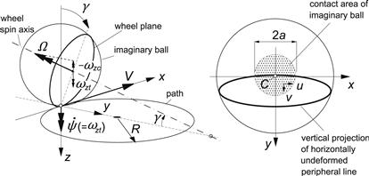
FIGURE 3.22 Wheel rolling at a camber angle while turning along a circular path without side slip. At the right: a top view of the peripheral line of the nonrolling wheel considered as being a part of an imaginary ball pressed against a flat surface.
We apply the theory of a rolling and slipping body and consider Eqns (2.55, 2.56) and restrict ourselves to the case of steady-state pure spin, that is, with α = κ = 0. Then with turn slip velocity ωzt = ![]() in Figure 3.22, we find
in Figure 3.22, we find
![]() (3.53)
(3.53)
Furthermore, the difference between (x, y) and (xo, yo) will be neglected and tire conicity and ply-steer disregarded. The correction factors θ attributed to camber may be approximated by
![]() (3.54)
(3.54)
with both reduction factors ε equal or close to zero for a railway wheel or a motorcycle tire and expected to be closer to unity for a steel belted car or truck tire, cf. discussion below Eqn (3.117). With both factors assumed equal and denoted as εγ, we may define a total actual spin
![]() (3.55)
(3.55)
The last term represents the curvature −1/Rγ of the tire peripheral line touching a frictionless surface at a cambered position. When disregarding a possible uniform offset of this line, we obtain, when integrating (2.52) by using (3.54) and approximating (2.51) by taking ![]() ,
,
![]() (3.56)
(3.56)
which reduces expressions (2.55, 2.56) for the sliding velocities with (3.53–55) to
 (3.57)
In the range of adhesion where the sliding velocities vanish, the deflection gradients become
![]() (3.58)
(3.58)
Integration yields the following expressions for the horizontal deformations in the contact area:
![]() (3.59)
(3.59)
The second expression is, of course, an approximation of the actual variation which is according to a circle. The approximation is due to the assumption made that the deflections v are much smaller than the path radius R. The constants of integration follow from boundary conditions which depend on the tire model employed and on the slip level. As an example, consider the simple brush model with horizontal deformations through elastic tread elements only. The contact area is assumed to be rectangular with length 2a and width 2b and filled with an infinite number of tread elements. In Figure 3.23, three rows of tread elements have been shown in the deformed situation. For this model, the following boundary conditions apply:
![]() (3.60)
(3.60)
with the use of (3.59), the formulas for the deformations in the adhesion zone starting at the leading edge read
![]() (3.61)
(3.61)
After introducing ![]() and
and ![]() denoting the stiffness of the tread rubber per unit area in x- and y-direction respectively and assuming small spin and hence vanishing sliding, we can calculate the lateral force and the moment about the vertical axis by integration over the contact area. We obtain
denoting the stiffness of the tread rubber per unit area in x- and y-direction respectively and assuming small spin and hence vanishing sliding, we can calculate the lateral force and the moment about the vertical axis by integration over the contact area. We obtain
 (3.62)
or, in terms of path curvature (if α ≡ 0 or constant) and camber angle (γ small),
 (3.63)
In the case of pure turning, the force acting on the tire is directed away from the path center and the moment acts opposite to the sense of turning. Consequently, both the force and the moment try to reduce the curvature 1/|R|. In the case of pure camber, the force on the wheel is directed toward the point of intersection of the wheel axis and the road plane, while the moment tries to turn the rolling wheel toward this point of intersection. No resulting force or torque is expected to occur when (1 − εγ) sin γ = re/R. For the special case that εγ = 0, this will occur when the point of intersection and the path center coincide. As the lateral deflection shows a symmetric distribution, the moment must be caused solely by the longitudinal forces. The generation of the moment may be explained by considering three wheels rigidly connected to each other, mounted on one axle. The wheels rotate at the same rate but in a curve the wheel centers travel different distances in a given time interval and, when cambered, these distances are equal but the effective rolling radii are different. In both situations, opposite longitudinal slip occurs, which results in a braked and a driven wheel (in Figure 3.23 the right- and the left-hand wheel respectively) and consequently in a couple Mz.
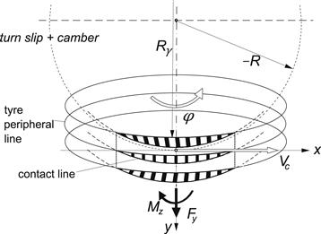
FIGURE 3.23 Top view of cambered tire model rolling in a curve with radius −R.
Up to now we have dealt with the relatively simple case of complete adhesion. When sliding is allowed by introducing a limited value of the coefficient of friction μ, the calculations become quite complicated. When a finite width 2b is considered, complete adhesion will only occur for vanishing values of spin. We expect that sliding will start at the left and right rear corners of the contact area, since in these points the available horizontal contact forces reduce to zero and the longitudinal deformations u would become maximal in the hypothetical case that μ → ∞. The zones of sliding grow with increasing spin and will thereby cause a less than proportional variation of Fy and Mz with φ. The case of finite contact width is too difficult to handle by a simple analysis. It will be dealt with later on in Section 3.3 when the tread element following simulation method is introduced.
For now we assume a thin tire model with b = 0. If, as before, a parabolic pressure distribution is assumed with a similar variation of the maximum possible lateral deflection vmax, it is obvious from Eqn (3.61) showing that the lateral deflection is also (approximately) parabolic that no sliding will occur up to a certain critical value of spin φsl, where the adhesion limit is reached throughout the contact length. Up to this point, Fy varies linearly with φ and Mz remains equal to zero.
According to Eqn (3.63) with εγ assumed to take a value that is minimally equal to zero, spin due to camber theoretically cannot exceed the value 1/re. Consequently, at larger values of spin turn slip must be involved. Beyond the critical value φsl the situation becomes quite complex. The discussion may be simplified by considering a turntable on top of which the wheel rolls with its spin axis fixed. The condition of adhesion is satisfied when the deflections remain within the boundaries given by the parabola’s ±vmax as indicated in Figure 3.24a. In the same figure, the corresponding situation at camber has been indicated at the same value of spin with curvature 1/Rγ of the deflected peripheral line (yγo, Eqn (3.56)) on a μ = 0 surface equal to the path curvature 1/R.
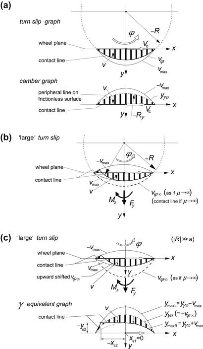
FIGURE 3.24 The tire brush model with zero width rolling while turning or at a camber angle (a) at full adhesion. Turning at large spin showing sliding at the front half and at the rear end (b,c), with parabolic approximation of the circular path in (c).
Sliding occurs as soon as the points of the table surface can cross the adhesion boundary ±vmax. This occurs simultaneously for all the points in the front half of the contact line when the path curvature exceeds the curvature of the adhesion boundary. Once the contact point arrives in the rear half of the contact zone (at x = 0), the point can maintain adhesion because now the point on the table moves toward the inside of the adhesion boundaries. The point follows a circle until the opposite boundary is reached at x = xs2 (cf. Figure 3.24b,c) where the deformation v is opposite in sign and reaches its maximum value vmax, after which sliding occurs again. With increasing turn slip φ (= −1/R), this latter sliding zone grows. At the same time, the side force Fy decreases and the torque Mz, that arises for φ > φsl, increases until the situation is reached where R and Fy approach zero and Mz attains its maximum value (tire standing still and rotating about its vertical axis). In Figure 3.24c the radius R has been considered large with respect to half the contact length a. Then the circle segments may be approximated by parabolas which make the analysis a lot simpler. In the lower part of the figure, a camber equivalent graph has been depicted. The curved contact line in the adhesion range is then converted to a straight (horizontal) line. The graph is obtained from the turn slip graph by subtracting from all the curves the deflection vφ∞ that would occur if full adhesion can be maintained (e.g., at μ → ∞). We use this graph as the basis for the calculation of the force and moment response to spin: first for the case of pure spin and then for the case of combined spin and side slip.
The parameter θy defined by Eqn (3.6) is used again and the maximum possible lateral deflection reads according to (3.5):
![]() (3.64)
(3.64)
The deflection at assumed full adhesion would become
![]() (3.65)
(3.65)
Equating the deflection at full sliding to the one at full adhesion yields the spin at the verge of sliding:
![]() (3.66)
(3.66)
The locations of the transition points indicated in Figure 3.24c are found to be given by the coordinates:
 (3.67)
The deflections become in the first and second sliding regions and in the adhesion region respectively:
![]() (3.68)
(3.68)
Integration over the contact length yields, for the side force,
![]() (3.69)
(3.69)
and, for the moment,
![]() (3.70)
(3.70)
At φ = φsl, the force reduces to μFz sgn φ and the moment to zero. The same can be obtained from the expressions (3.62) holding for the case of full adhesion when 2 ![]() is replaced by
is replaced by ![]() and the width 2b is taken equal to zero.
and the width 2b is taken equal to zero.
For spin approaching infinity, that is when the radius R → 0, the force Fy vanishes while the moment reaches its maximum value:
![]() (3.71)
(3.71)
In Figure 3.25, the pure spin characteristics have been presented according to the above expressions. It is of interest to note that although the parabola does not resemble the circular path so well at smaller radii, the resulting response seems to be acceptable at least if the deflections remain sufficiently small.
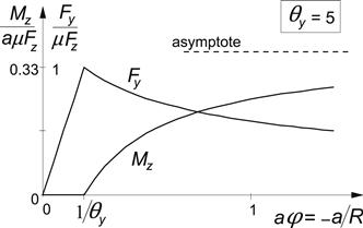
FIGURE 3.25 Force and moment vs nondimensional spin for single row brush model.
Spin and Side Slip
In the analysis of combined spin and side slip, we may distinguish again between the cases of small and large spin. As before, at small spin we have only a sliding range that starts at the rear end of the contact line, whereas at large spin we have an additional sliding zone that starts at the leading edge. First we will consider the simpler case of small spin.
In Figure 3.26, an example is shown of the single row brush model, both for the cases of turning and (equivalent) camber. In the camber graph, the curvesymaxL and ymaxR have been drawn which indicate the maximum possible displacements of the tips of the elements to the left and to the right with respect to the yγo line. The shaded area corresponds to the deformation of the brush model when subjected solely to the slip angle with the maximum possible deflection −vmax replaced by (in this case with negative slip angle) ymaxL. This would correspond to the introduction of an adapted friction coefficient μ or parameter θy. Apparently, the actual deflection of the elements at camber and side slip is then obtained by adding the deflection vφ∞ that would occur when the model would be subjected to spin only and full adhesion is assumed. The adapted parameter θy turns out to read
![]() (3.72)
(3.72)
with the condition for the spin to be ‘small’:
![]() (3.73)
(3.73)
The side force becomes similar to Eqn (3.11) with the camber force at full adhesion added:
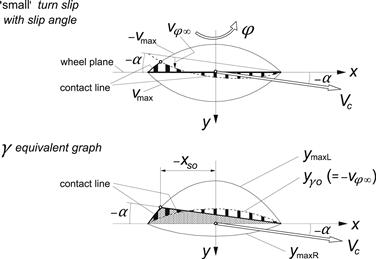
FIGURE 3.26 The brush model turning at ‘small’ spin or subjected to camber at the same level of spin while running at a slip angle.
if ![]()
![]() (3.74)
(3.74)
and if ![]()
![]() (3.74a)
(3.74a)
if ![]()
![]() (3.75)
(3.75)
and if ![]()
![]() (3.75a)
(3.75a)
We may introduce a pneumatic trail tα that multiplied with the force Fyα due to the slip angle (with the last term of (3.74) omitted) produces the moment −Mz:
if ![]()
 (3.76)
and else tα = 0.
The graph of Figure 3.27 clarifies the configuration of the various curves and their mutual relationship. For different values of the camber angle γ, the characteristics for the force and the moment versus the slip angle have been calculated with the above equations and presented in Figure 3.28. The corresponding Gough plot has been depicted in Figure 3.29. The relationship between γ and the spin φ follows from Eqn (3.55).
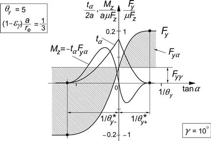
FIGURE 3.27 Basic configuration of the characteristics vs side slip at camber angle γ = 10°.
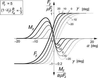
FIGURE 3.28 The calculated side force and moment characteristics at various camber angles.
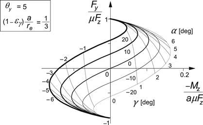
FIGURE 3.29 The corresponding Gough plot.
The curves established show good qualitative agreement with measured characteristics. Some details in their features may be different with respect to experimental evidence. In the next section where the simulation model is introduced, the effect of various other parameters like the width of the contact patch and the possibly camber-dependent average friction coefficient on the peak side force will be discussed.
The next item to be addressed is the response to large spin in the presence of side slip. Figures 3.30a,b refer to this situation. Large spin with two sliding ranges occurs when the following two conditions are fulfilled:
![]() (3.77)
(3.77)
If the second condition is not satisfied, we have a relatively large slip angle and the Eqns (3.74, 3.75) hold again. This situation is illustrated in Figure 3.30c.
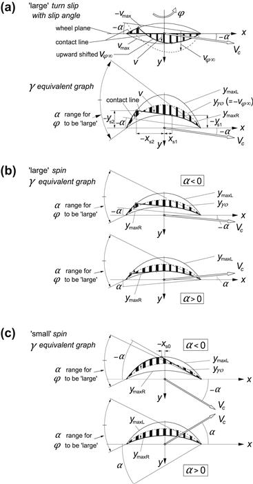
FIGURE 3.30 The model running at large spin (turning and equivalent camber) at a relatively small (a, b) or large positive or negative slip angle (c).
For the development of the equations for the deflections, we refer to Figure 3.30a with the camber equivalent graph. First, the distances y will be established and then the deflections vφ∞ will be added to obtain the actual deflections v. Adhesion occurs in between the two sliding ranges. The straight line runs parallel to the speed vector and touches the boundary ymaxR. The tangent point forms the first transition point from sliding to adhesion. More to the rear, the straight line intersects the other boundary ymaxL. With the following two quantities introduced,
![]() (3.78)
(3.78)
we derive for the x-coordinates of the transition points:
![]() (3.79)
(3.79)
and
![]() (3.80)
(3.80)
with
![]() (3.81)
(3.81)
The distances y in the first sliding region (xs1 < x < a) read
![]() (3.82)
(3.82)
in the adhesion region (xs2 < x < xs1):
![]() (3.83)
(3.83)
with
![]() (3.84)
(3.84)
and in second sliding range (−a < x < xs2):
![]() (3.85)
(3.85)
Integration over the contact length after addition of vφ∞ and multiplication with the stiffness per unit length cpy gives the side force and after first multiplying with x the aligning torque. We obtain the formulas
 (3.86)
 (3.87)
The resulting characteristics have been presented in Figures 3.31 and 3.32. The graphs form an extension of the diagram of Figure 3.28 where the level of camber corresponds to ‘small’ spin. It can be observed that in accordance with Figure 3.25 the force at zero side slip first increases with increasing spin and then decays. As was the case with smaller spin for the case where spin and side slip have the same sign, the slip angle where the peak side force is reached becomes larger. When the signs of both slip components have opposite signs, the level of side slip where the force saturates may become very large. As can be seen from Figure 3.30b, the deflection pattern becomes more anti-symmetric when with positive spin the slip angle is negative. This explains the fact that at higher levels of spin, the torque attains its maximum at larger slip angles with a sign opposite to that of the spin. The observation concerning the peak side force, of course, also holds for the slip angle where the torque reduces to zero.
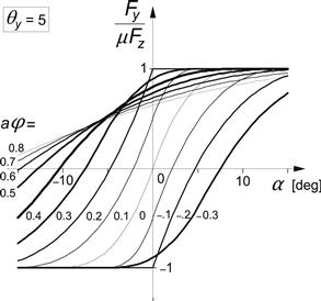
FIGURE 3.31 Side force characteristics of the single row brush model up to large levels of spin (compare with Figure 3.28 where spin is small and aφ = 0.33 sin γ).
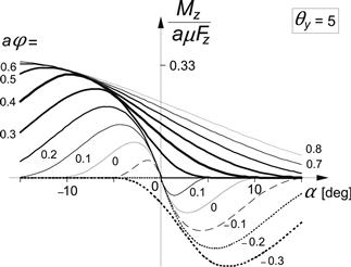
FIGURE 3.32 Aligning torque characteristics of the single row brush model up to large levels of spin (compare with Figure 3.28 where spin is small and aφ = 0.33 sin γ).
Spin, Longitudinal and Side Slip, the Width Effect
The width of the contact patch has a considerable effect on the torque and indirectly on the side force because of the consumption of some of the friction by the longitudinal forces involved. Furthermore, for the actual tire with carcass compliance, the spin torque will generate an additional distortion of the carcass which results in a further change of the effective slip angle (beside the distortion already brought about by the aligning torque that results from lateral forces). Among other things, these matters can be taken into account in the tread simulation model to be dealt with in Section 3.3.
In the part that follows now, we will show the complexity involved when longitudinal slip is considered besides spin and side slip. To include the effect of the width of the contact patch, we consider a model with a left and a right row of tread elements positioned at a distance yL = −brow and yR = brow from the wheel center plane. In fact, we may assume that we deal with two wheels attached to each other on the same shaft at a distance 2brow from each other. The wheels are subjected to the same side slip and turn slip velocities, Vsy and ![]() , and show the same camber angle γ. However, the longitudinal slip velocities are different for the case of camber because of a difference in effective rolling radii. We have, for the longitudinal slip velocity of the left or right wheel positioned at a distance yL,R from the center plane,
, and show the same camber angle γ. However, the longitudinal slip velocities are different for the case of camber because of a difference in effective rolling radii. We have, for the longitudinal slip velocity of the left or right wheel positioned at a distance yL,R from the center plane,
![]() (3.88)
(3.88)
This expression is obtained by considering Eqn (2.55) in which conicity is disregarded, steady-state is assumed to occur and the camber reduction factor εγ is introduced. The factors θ are defined as (like in (3.54, 3.55))
![]() (3.89)
(3.89)
From Eqns (2.55, 2.56) using (3.88), the sliding velocity components are obtained:
![]() (3.90)
(3.90)
![]() (3.91)
(3.91)
After introducing the theoretical slip quantities for the two attached wheels
![]() (3.92)
(3.92)
we find, for the gradients of the deflections in the adhesion zone (where Vg = 0) if small spin is considered (sliding only at the rear),
![]() (3.93)
(3.93)
![]() (3.94)
(3.94)
which yields after integration for the deflections in the adhesion zone (x < xt):
![]() (3.95)
(3.95)
![]() (3.96)
(3.96)
The transition point from adhesion to sliding, at x = xt, can be assessed with the aid of the condition
![]() (3.97)
(3.97)
with the magnitude of the deflection
![]() (3.98)
(3.98)
Solving for xt and performing the integration over the adhesion range may be carried out numerically. In the sliding range, the direction of the deflections varies with x. As an approximation, one may assume that these deflections e (for an isotropic model) are all directed opposite to the slip speed VsL,R. Results of such integrations yielding the values of Fx, Fy and Mz will not be shown here. We refer to Sakai (1990) for analytical solutions of the single row brush model at combined slip with camber.
3.3 The Tread Simulation Model
In this section, a methodology is developed that enables us to investigate effects of elements in the tire model which were impossible to include in the analytical brush model dealt with in the preceding Section 3.2. Examples of such complicating features are: arbitrary pressure distribution; velocity and pressure dependent friction coefficient; isotropic stiffness properties; combined lateral, longitudinal and camber or turn slip; lateral, bending and yaw compliance of the carcass and belt; and finite tread width at turn slip or camber.
The method is based on the time simulation of the deformation history of one or more tread elements while moving through the contact zone. The method is very powerful and can be used either under steady-state or time-varying conditions. In the latter nonsteady situation, we may divide the contact length into a number of zones of equal length in each of which a tread element is followed. In the case of turning or camber, the contact patch should be divided into several parallel rows of elements. While moving through the zones, the forces acting on the elements are calculated and integrated. After having moved completely through a zone, the integration produces the zone forces. These forces act on the belt and the corresponding distortion is calculated. With the updated belt deflection, the next passage through the zones is performed and the calculation is repeated.
Here, we will restrict the discussion to steady-state slip conditions and take a single zone with length equal to the contact length. In Section 2.5, an introductory discussion has been given and reference has been made to a number of sources in the literature. The complete listing of the simulation program TreadSim written in Matlab code can be found online (cf. App. 2). For details, we may refer to this program.
Figure 3.33 depicts the model with deflected belt and the tread element that has moved from the leading edge to a certain position in the contact zone. In Figure 3.34, the tread element deflection vector e has been shown. The tread element is assumed to be isotropic, thus with equal stiffnesses in the x- and y-direction. Then, when the element is sliding, the sliding speed vector Vg, that has a sense opposite to the friction force vector q, is directed opposite to the deflection vector e. The figure depicts the deflected element at the ends of two successive time steps i − 1 and i. The first objective is now to find an expression for the displacement g of the tip of the element while sliding over the ground.
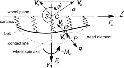
FIGURE 3.33 Enhanced model with deflected carcass and tread element that is followed from front to rear.
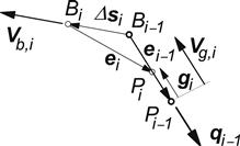
FIGURE 3.34 The isotropic tread element with deflection e in two successive positions i − 1 and i. Its base point B moves with speed Vb and its tip P slides with speed Vg.
The contact length is divided into n intervals. Over each time step Δt, the base point B moves over an interval length toward the rear. With given length
![]() (3.99)
(3.99)
and the linear speed of rolling Vr = reΩ, the time step Δt is obtained
![]() (3.100)
(3.100)
with the velocity vector Vb of point B, the displacement vector Δs of this point over the time step becomes
![]() (3.101)
(3.101)
The base point B moves along the belt peripheral line or a line parallel to this line. With the known lateral coordinate yb of this line of base points with respect to the wheel center plane, the local slope ![]() can be assessed. Then, with the slip velocity Vs of the slip point S, the yaw rate of the line of intersection
can be assessed. Then, with the slip velocity Vs of the slip point S, the yaw rate of the line of intersection ![]() , and the rolling speed Vr, the components of Vb can be found.
, and the rolling speed Vr, the components of Vb can be found.
The velocity of point B may be considered as the sliding velocity of this point with respect to the ground and we may employ equations (2.55, 2.56) for its assessment. In these equations, at steady state, the time derivatives of u and v vanish, the slope ![]() is replaced by zero, and for
is replaced by zero, and for ![]() we take the gradient of the belt deflection caused by the external force and moment. We have, with average x position xb = x + 0.5Δx,
we take the gradient of the belt deflection caused by the external force and moment. We have, with average x position xb = x + 0.5Δx,
![]() (3.102)
(3.102)
![]() (3.103)
(3.103)
with the slip and roll velocities
![]() (3.104)
(3.104)
The lateral displacement yb of the belt at the contact center is attributed to camber, conicity, and the lateral external force (through the lateral compliance of the carcass). The gradient ![]() may be approximately assessed by assuming a parabolic base line yb(xb) exhibiting an average slope cs influenced by the aligning torque (through the yaw compliance) and ply-steer, and a curvature cc influenced by the side force (through the bending stiffness) and camber and conicity (cf. (3.56)). We have, for the lateral coordinate,
may be approximately assessed by assuming a parabolic base line yb(xb) exhibiting an average slope cs influenced by the aligning torque (through the yaw compliance) and ply-steer, and a curvature cc influenced by the side force (through the bending stiffness) and camber and conicity (cf. (3.56)). We have, for the lateral coordinate,
![]() (3.105)
(3.105)
and, for its approximation used in (3.102),
![]() (3.106)
(3.106)
and the slope:
![]() (3.107)
(3.107)
Conicity and ply-steer will be interpreted here to be caused by ‘built-in’ camber and slip angles. These equivalent camber and slip angles γcon and αply are introduced in the expressions of the quantities θ. We define
![]() (3.108)
(3.108)
and
![]() (3.109)
(3.109)
The coefficients εγx and εγy may be taken equal to each other. The first term of the displacement (3.105) is just a guess. It constitutes the lateral displacement of the base line at the contact center when the tire is pressed on a frictionless surface in the presence of conicity and camber. The displacements at the contact leading and trailing edges are assumed to be zero under these conditions. The approximation ybo(3.106) is used in (3.102) to avoid apparent changes in the effective rolling radius at camber. The actual lateral coordinate yb (3.105) plus a term yrγ is used to calculate the aligning torque. With this additional term, the lateral shift of Fx due to sideways rolling when the tire is being cambered is accounted for. We have yb,eff = yb + yrγ with yrγ = εyrγ b sin γ with an upper limit of its magnitude equal to b. The moment ![]() causes the torsion of the contact patch and is assumed to act around a point closer to its center as depicted in Figure 3.19. A reduction parameter
causes the torsion of the contact patch and is assumed to act around a point closer to its center as depicted in Figure 3.19. A reduction parameter ![]() is used for this purpose. More refinements may be introduced to better approximate the shape of the base line, especially near the leading and trailing edges (bending back).
is used for this purpose. More refinements may be introduced to better approximate the shape of the base line, especially near the leading and trailing edges (bending back).
With the displacement vector Δs (3.101) established, we can derive the change in deflection e over one time step. By keeping the directions of motion of the points B and P in Figure 3.34 constant during the time step, an approximate expression for the new deflection vector is obtained. After the base point B has moved according to the vector Δs, we have
![]() (3.110)
(3.110)
Here, ei−1 denotes the absolute value of the deflection and gi, the distance P, has slided in the direction of −ei−1. In the case of adhesion, the sliding distance gi = 0. When the tip slides, the deflection becomes
![]() (3.111)
(3.111)
From (3.110), an approximate expression for gi can be established, considering that g is small with respect to the deflection e. We obtain
![]() (3.112)
(3.112)
in which expression (3.111) is to be substituted. If gi is positive, sliding remains. If not, adhesion commences. In the case of sliding, the deflection components can be found from (3.110) using (3.112). Then, the force vector per unit length is
![]() (3.113)
(3.113)
If adhesion occurs, gi = 0 and with (3.110) the deflection is determined again. The force per unit length now reads
![]() (3.114)
(3.114)
As soon as the condition for adhesion
![]() (3.115)
(3.115)
is violated, sliding begins. The sliding distance gi is calculated again and its sign checked until adhesion may show up again.
In (3.113), the friction coefficient appears. This quantity may be expressed as a function of the sliding velocity of the tip of the element over the ground. However, this velocity is not available at this stage of the calculation. Through iterations, we may be able to assess the sliding speed at the position considered. Instead, we will adopt an approximation and use the velocity of the base point (3.102, 3.103) to determine the current value of the friction coefficient. The following functional relationship may be used for the friction coefficient versus the magnitude of the approximated sliding speed Vb:
![]() (3.116)
(3.116)
During the passage of the element through the contact zone, the forces ΔFi are calculated by multiplying qi with the part of the contact length Δx covered over the time step Δt.
Subsequently, the total force components and the aligning moment are found by adding together all the contributions ΔFxi, ΔFyi, and xbiΔFyi−ybi,effΔFxi, respectively. A correction to the moment arm may be introduced to account for the side ways rolling of the tire cross section while being cambered and deflected (causing lateral shift of point of action of the resulting normal load Fz and similarly of the longitudinal force Fx). Also, the counter-effect of the longitudinal deflection uc may contribute to this correction factor (cf. Eqn (3.51)).
For details and possible application of the model, we refer to the complete listing of the Matlab program TreadSim presented online.
In the sequel, a number of example results of using the tread simulation model have been presented. The following cases have been investigated:
1. Sliding velocity-dependent friction coefficient (rigid carcass but parameter c of Eqn (3.52) is included) (Figure 3.35a).
2. Flexible carcass, without and with camber (Figure 3.35b).
3. Finite tread width (two rows of tread elements, flexible carcass), with and without camber (Figure 3.35c).
4. Combined lateral and turn slip (two rows, flexible carcass) (Figure 3.35d).
5. Pneumatic trail at pure side slip (flexible and rigid carcass) (Figure 3.36).
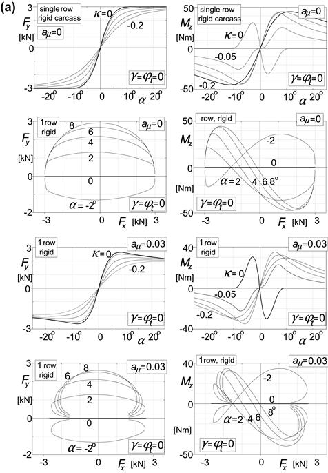
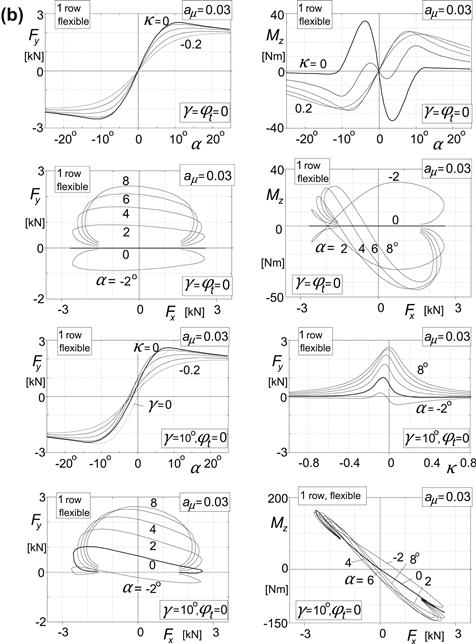
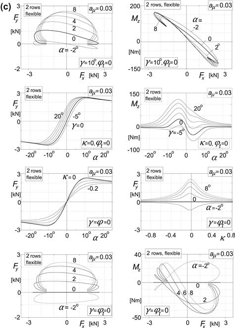
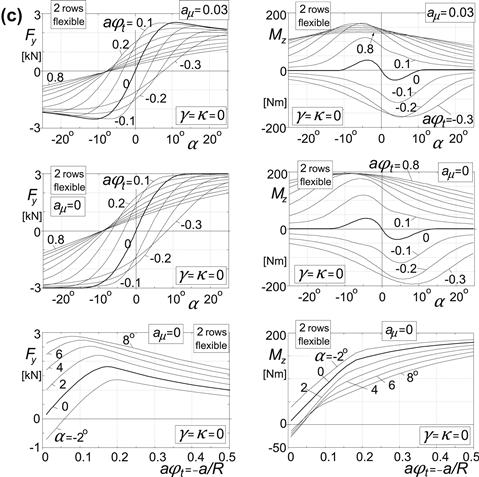
FIGURE 3.35(a) Characteristics computed with tread simulation model.
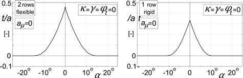
FIGURE 3.36 Pneumatic trail variation as computed with tread simulation model.
The computations have been conducted with the set of parameter values listed in Table 3.1.
TABLE 3.1 Parameter Values used in the Tread Simulation Model (Figures 3.35–3.37)
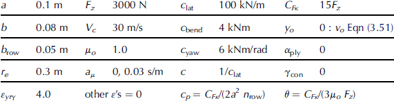
In the case of a ‘rigid’ carcass, parameter c (= 0.01 m/kN), Eqn (3.52), is used while clat, cbend, cyaw → ∞. As indicated, quantities cp and θ follow from the model parameters.
The graphs of the lower half of Figure 3.35a relative to the upper half show the most prominent effect of a with sliding velocity decreasing friction coefficient. At aμ = 0.03, the side force Fy exhibits a clear peak at a slip angle of about seven degrees when the wheel is rolling freely (κ = 0). Also, the fore-and-aft force Fx tends to decrease after having reached its peak value. The inward endings of the curves at constant values of slip angle shown in the bottom diagram are typical especially for a tire running on wet road surfaces. The peak values themselves will decrease when the speed of travel is increased (not shown) while the initial slopes (slip stiffnesses) remain unchanged. The change in sign of the aligning torque in the braking range of its diagram occurs because of the retained parameter c that produces the effect of the flexible carcass according to Eqns (3.51, 3.52). The expected change in sign of the aligning torque curve at pure side slip at higher levels of side slip does not occur due to the limitation of the estimation of the sliding speed for which the speed of a point of the belt is taken (here rigid). In Figure 3.35b with the carcass considered flexible, this sign change does show up as illustrated in the upper right diagram.
A more important effect of the flexible carcass presented in Figure 3.35b is the decreased cornering stiffness while the fore-and-aft slip stiffness remains the same. The lower value of Fy at α = 2° in the Fy vs Fx diagram clearly demonstrates this effect (the curves become less curved). The aligning torque, however, is not so much affected. This is due to the larger pneumatic trail which is a result of the curved deflection line of the belt. Figure 3.36 shows the pneumatic trail diagram for the model with and without carcass compliance (the number of rows has no influence in case of zero spin). As expected, the simple brush model with rigid carcass has a trail of 0.33a when the slip angle approaches zero. The flexible carcass model considered features a pneumatic trail of about 0.46a. See Figure 3.38 for the deflection pattern.
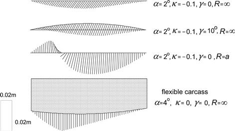
FIGURE 3.38 Examples of deflection patterns at various combinations of slip for the single row model with rigid and flexible carcass.
The influence on the curves of the introduction of the relatively large camber angle of 10° is indicated in the lower half of Figure 3.35b. The effect is most clearly demonstrated in the lower-left diagram. The camber thrust is accompanied by a lateral deflection that causes a shift of the line of action of the longitudinal force. The resulting torque tends to rotate the lower part of the belt about the vertical axis which now can be accomplished through the yaw compliance of the carcass. At braking, the rotation is such that an apparent slip angle arises that increases the camber side force. At driving, the opposite occurs. As a result, the constant slip angle curves plotted in the diagram show an inclination. The corresponding influence diagram of κ on Fy shows distorted curves when compared with those of Figure 3.11. The inversed S shape of the curves at small slip angle is a feature that is commonly encountered in measured characteristics. The aligning torque diagram (lower-right picture) is considerably changed as a result of the action of the torque mentioned above that originates from Fx.
In Figure 3.35c, the effect of a finite width of the contact patch is demonstrated. Two rows of tread elements have been considered. At the camber angle of 10°, a spin torque is generated that appears to rotate the lower part of the belt in such a way that an apparent slip angle arises that increases the camber thrust. The upper-left-hand diagram shows the increase in side force. The right-hand diagram indicates the considerable rise in the aligning torque as a result of the spin torque in the range of small longitudinal force Fx.
The two diagrams in the second row demonstrate the effects of tread width, carcass flexibility, and friction decay with velocity on the side force and moment vs slip angle characteristics for a series of camber angles. The plots may be compared with those of Figure 3.28. The lower half of Figure 3.35c refers to the case without camber and may be compared with the plots of the upper half of Figure 3.35b that does not include the effects of tread width.
Figure 3.35d presents the force and moment characteristics for a series of levels of turn slip, including large values of spin corresponding to a radius of curvature equal to a/0.8. The figures of the second row refer to the case of constant friction (aμ = 0) and may be compared with Figures 3.31, 3.32. An interesting effect of tread width is the further decrease of the side force at higher levels of turn slip due to longitudinal slip that occurs on both sides of the contact patch which consumes a lot of the available frictional forces. Of course, the aligning torque is now considerably larger. The third row of diagrams represents the spin force and moment characteristics at various levels of side slip. In Figure 3.37, the pure spin characteristics have been drawn for the model with a rigid carcass provided with one row of tread elements (same as Figure 3.25) and with two rows computed with the tread simulation model. Comparison clearly shows the considerable reduction of the peak side force and the much larger level of the aligning torque caused by the finite tread width. The influence of carcass flexibility appears to be very small both for the force and for the moment.
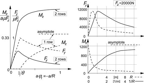
FIGURE 3.37 Pure turn slip characteristics according to the model (left, rigid carcass with one or two rows of elements) and results from experiments with a bias-ply truck tire (right, 9.00–20 eHD, pi = 5.5 bar, V = 1–3 km/h on dry road, from Freudenstein 1961). Model parameters: θ = 5, aμ = 0, and brow = 0.5 a.
These results indicate that the single row theory developed in Section 3.2 also for high spin in combination with side slip has only limited practical significance. The influence of small spin, i.e., camber, on the side force vs slip angle characteristic as calculated with the aid of the simple single row, rigid carcass brush model may be considered as reasonable.
Freudenstein (1961) has conducted side-slip and turning experiments with a bias-ply truck tire on a dry road surface. The side-slip measurement results of this tire were already depicted in Figure 3.6. In the right-hand diagram of Figure 3.37, the results from the turning experiments have been presented. As abscissa, both the path radius and the path curvature have been used. Obviously, the calculated two-row model characteristics show good qualitative agreement with the experimental curves. For the values a = 0.1 m, μFz = 20000 N, and θ = 8, a very reasonable also quantitative correspondence for both the force and the moment characteristics of Figure 3.37 can be obtained. Freudenstein suggests the following formula for the peak moment generated at pure turning at wheel speed V = 0:
![]() (3.117)
(3.117)
As Freudenstein did not give the camber characteristics of the truck tires on which the turning behavior was measured, we are not able to compare the responses to camber and turning. According to Hadekel (1952), for aircraft tires the lateral force due to turning is about four times higher than the camber force at equal values of spin. From experiments performed by Higuchi (1997), a factor of about two can be deduced for a radial ply car tire (cf. Chap. 7 discussion above Figure 7.11). This supports the theory of the reduced curvature of the peripheral line of the cambered tire pressed on a frictionless surface due to the high lateral bending stiffness of the tread band, as illustrated in Figure 2.10, and the associated coefficient εγ in Eqn (3.55). The program TreadSim also provides information on the distribution of contact forces and deflections of belt and tread elements. Some examples of the deformation pattern have been depicted in Figures 3.38 and 3.39. In Figure 3.38, the deflections of the single row brush model have been depicted and in addition of the model with carcass lateral, yaw and bending compliance. As indicated, the scale of the drawing has been chosen larger in lateral direction. In the middle two diagrams, the influence of camber and of turning on the deflections at side and brake slip has been shown. Turning was considered with an exceptionally small turn radius R equal to a which is half the contact length. One may note the central section where adhesion occurs. The latter situation also occurs with the middle row of tread elements of the three row brush model depicted in Figure 3.39. In this drawing, the scales are the same. Clearly, the tire generates longitudinal deflections of the outer rows of elements which contribute to the torque.
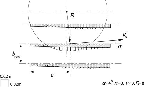
FIGURE 3.39 Deflections of the tread elements and of the belt for the three row model at side slip and turning.
3.4 Application: Vehicle Stability at Braking up to Wheel Lock
When the vehicle is being braked forcefully and a possible downward slope does not compensate for the reduction in speed of travel, the situation can no longer be considered as steady state. The influence of the rate of change of the longitudinal speed and of the effect of combined slip on the lateral stability may no longer be neglected. Instead of using the two first-order differential equations (1.42) for the lateral and yaw motions, we must now consider the complete set, including the equation for the longitudinal motion which is also of the first order.
Because of the complexity involved, the influence of the height of the center of gravity on the vehicle motion will be disregarded. With a finite height, fore-and-aft but also lateral load transfer would occur, the latter causing unequal braking forces on the left- and right-locked wheels that give rise to a stabilizing torque counteracting the effect of the fore and aft load transfer.
The steer angle is kept equal to zero. This two-wheel, single-track, rigid vehicle with zero c.g. height has been depicted in Figure 3.40 where the wheel on axle 2 is considered to be locked. For the three states, we obtain the equations
 (3.118)
with
 (3.119)
and
![]() (3.120)
(3.120)
For a proper simulation of the motion, the slip ratio’s κi should result from the wheel speeds of revolution Ωi which would require additional degrees of freedom. For this occasion, we will employ an alternative approach that involves the introduction of functions for the side force in which its direct dependence on the braking effort (or brake pressure) is included. This is possible when ‘dry’ friction is assumed to occur between tire and road and the curves of the right-most diagram of Figure 1.2 do not show inward endings and thus double valued functions are avoided. The characteristics of Figure 3.16 will be used for our analysis. In Figure 3.41, the characteristics have been reproduced: one curve for the freely rolling wheel, another one for the wheel that is being braked with a braking effort corresponding to a brake force B1 = −Fx1 at straight ahead rolling (α small) and finally for a wheel that is locked completely. The second curve shows that at higher slip angles, a lower horizontal plateau is followed until the straight inclined line is reached where also this wheel gets locked (note that sin α has been used as abscissa which makes the relationship linear). A full discussion of this behavior has been given in Subsection 3.2.3 in connection with the treatment of the tire brush model.
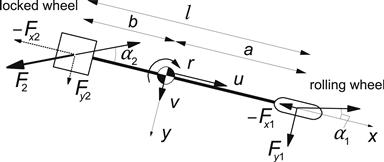
FIGURE 3.40 ‘Bicycle’ model with one wheel locked.
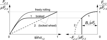
FIGURE 3.41 Tire side force characteristics for freely rolling and braked wheels.
As shown in Figure 3.40, we assume that the wheel on axle 2 is locked and that on axle 1 may be braked. The characteristics of Figure 3.41 apply. First, the situation near the undisturbed straight ahead motion will be studied. Linearization with both slip angles assumed small yields for the horizontal wheel forces:
 (3.121)
For the locked wheel, we have now an effective side-slip stiffness:
![]() (3.122)
(3.122)
As a result, Eqns (3.118–3.120) reduce to
 (3.123)
Furthermore, we have introduced the absolute value of the forward speed u in the denominators to allow for the consideration of negative values of u, while at the same time the sign of α remains unchanged (cf. the corresponding equations (1.46) for the nondriven or braked vehicle). Negative values of u correspond to the case of locked front wheels.
Elimination of the lateral velocity v from Eqn (3.123) yields
![]() (3.124)
(3.124)
When compared with Eqn (1.50), considering (1.48), it is noted that in the second coefficient of (3.124), the term k2C2 has disappeared and that −k2B1 has been added. This is due to the differentiation of u in the elimination process of v. We had, originally in the second coefficient of (3.124), the term
![]() (3.125)
(3.125)
which explains the changes observed. In other respects, Eqn (3.124) is similar to the homogeneous version of Eqn (1.50). However, an important difference appears in the coefficients which are now dependent on the time because of the presence of the linearly with time decreasing speed u. We have the additional equation for u (by integration of the first of Eqn (3.123)):
![]() (3.126)
(3.126)
The exact solution of Eqn (3.124) can be found because of the fortunate fact that the equation can be reduced to the differential equation of Bessel, the solution of which is known in tabular form. Before giving an example of such a complete solution, we will analyze the motion just after the application of a slight disturbance which allows us to approximate the equation to one with constant parameters in which u is replaced by its initial value uo. For this substitutive equation, the solution can be found easily. We obtain
![]() (3.127)
(3.127)
with D1,2 denoting the constants of integration (governed by the initial values of the state variables v and r) and λ1,2 representing the eigenvalues, that is, the roots of the characteristic equation of the substitutive differential equation:
![]() (3.128)
(3.128)
Comparison with the coefficients of Eqn (3.124) reveals the expressions for the quantities A, B, C, and D. Since, apparently, the first three are always positive and in the case considered C2 is much smaller than C1 which makes D also a positive quantity, we expect that the substitutive system can only become unstable because of a possibly negative third coefficient. Then, one of the roots (lets say λ1) becomes positive (while remaining real). Obviously, this can only occur when u is positive which means: when the wheels of the rear axle are locked. Locked front wheels which occur when in our system description u < 0 will not destabilize the system but makes the vehicle unsteerable. This is because of the fact that changing the steer angle of a locked wheel cannot effect the orientation of its frictional force vector. The car with locked rear wheels corresponds in behavior with the case of excessive oversteer while locked front wheels would give rise to extreme understeer. The critical speed for the case of locked rear wheels is derived by making the third coefficient of Eqn (3.128), or of Eqn (3.124), equal to zero. We find, by using (3.122),
 (3.129)
From this expression, it can be seen that when a rigid front tire is considered so that C1 → ∞, we obtain the simple form: ![]() . The influence of an elastic front tire is not very great as the front cornering stiffness may range from 6 to 30 times the tire normal load. Considering a dry road with μ = 1, we find a critical speed of about 20 km/h.
. The influence of an elastic front tire is not very great as the front cornering stiffness may range from 6 to 30 times the tire normal load. Considering a dry road with μ = 1, we find a critical speed of about 20 km/h.
In view of this very low speed above which the vehicle with rear wheels locked becomes unstable and the fact that normally the speed will already be a lot larger than the critical speed when the brakes are being applied, it is more useful to consider the degree of instability as a function of speed. We will adopt the root λ1 to represent the degree of instability. Figure 3.42 illustrates the manner in which the roots vary with speed of travel. The diagram includes the case of front wheels locked (u < 0), where obviously the roots remain negative and become complex at higher speeds of travel (real part: dotted curve). As a practical indication for the degree of instability, we may employ the height of the horizontal asymptote to which λ1 tends when u → ∞. For that we find
![]() (3.130)
(3.130)
which shows that instability decreases when the front tire cornering stiffness is lower and becomes more in balance with the here very low rear ‘cornering stiffness’ (3.122). It also becomes clear that when the front wheels are locked as well (C1 = μFz1), the degree of instability reduces to zero representing indifferent stability.
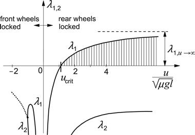
FIGURE 3.42 Real (part of the) eigenvalues of the substitutive linear system with constant coefficients.
The complete solution of Eqn (3.124) can be found by applying the Lommel transformation of the Bessel differential equation and using the modified functions of Bessel in its solution. These functions are available in tabulated form and can be found in the book by Abramowitz and Stegun (1965, cf. Eqn 9.1.53 for the transformed equation and p. 377 for the solution).
In the paper of Koiter and Pacejka (1969), the exact solution has been given together with examples of the numerically computed solution for the complete nonlinear system. For the special case with parameters a = b = k, B1 = 0, C1/μFz = 6, the solution of the linear Eqn (3.124) is presented in Figure 3.43. The exact solution is compared with the approximate one (3.127) of the substitutive equation. The solution in the form of a stable and an unstable branch has been drawn in the (u, r) plane constituting the projection of the complete three-dimensional trajectory in the (u, v, r) space. Along the u axis, we may introduce the time axis considering the relationship (3.126). In the case considered the nondimensional eigenvalues λ1,2√(l/μg) take the values 1.26 and −3.43 respectively. For the sake of comparison, the initial values have been taken the same for both pairs of solutions. No visible difference can be detected between the two decaying stable branches. The ‘unstable’ branch of the exact solution, however, shows for greater values of time an increasing difference with the corresponding approximate exponential solution. At the start of the motion where the rear axle tends to break away the agreement is very good. It can be shown that when expanded in a series of powers of the time t, the solutions are identical up to and including the third term (with t2). This supports our choice of defining the degree of instability.
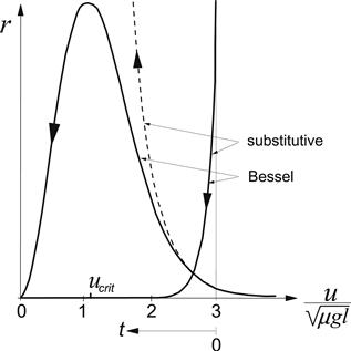
FIGURE 3.43 Solutions of the exact and the approximated linear systems representing the variation of the yaw rate r with forward velocity u or with time t.
Along the vertical axis, the yaw rate is plotted. After having attained a maximum, the yaw angle develops at a lesser rate until the motion reaches a complete stop. The area underneath the curves is proportional to the final angle of swing. This finite angle will linearly depend on the initial values of the variables r and v. Consequently, the final deviation with respect to the original rectilinear path can be kept within any chosen limit and, strictly speaking, the actual system is always stable.
Finally, the solutions for the nonlinear system governed by the Eqns (3.118, 3.119) and tire characteristics according to Figure 3.41 have been established by numerical integration of the equations of motion. Now, the character of the motion may change with the level of the initial disturbance. In Figures 3.44 and 3.45, the resulting motions for two cases have been depicted: the first without braking the front wheels (Figure 3.44) and the second with also the front wheels being braked but at a lower effort to make sure that they roll at least initially. The initial speed of travel and disturbances has been kept the same for all cases but the coefficient of friction μ has been varied. At lower friction, the time available to develop the angle of swing is larger and we see that an angle of more than 180 degrees may be reached. Then the locked wheels are moving at the front (u < 0) and we have seen that situation is stable while the motion can become oscillatory (cf. Figure 3.42). For the case of Figure 3.44 with μ = 0.25, we indeed observe that a sign change occurs once for the yaw rate r. When the brakes are applied also at the front axle, the deceleration is larger and we have less time to come to a stop. Consequently, the final angles of Figure 3.45 are smaller than those reached in Figure 3.44. The shaded zones indicate the ranges where also the front wheels get locked. This obviously occurs when the slip angle of the initially rolling wheels 1 becomes sufficiently large and exceeds the value indicated in Figure 3.41 where the inclined straight line is reached. It has been found (not surprisingly) that the influence of raising the initial speed is qualitatively the same as the effect of reducing the coefficient of friction.
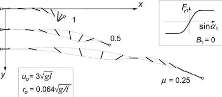
FIGURE 3.44 Development of the vehicle motion after the rear wheels get locked while the front wheels remain rolling freely.
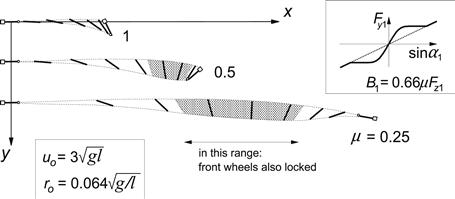
FIGURE 3.45 Development of the vehicle motion after the rear wheels get locked while also the front wheels are being braked.