4.2.1 Water Salinity

The salinity of water comprises the amount of solid matter in grams per kilogram of seawater when the bromine and iodine have been replaced by the equivalent chlorine, and when the carbonate has become oxide and the organic matter has been oxidized completely. In Table 4.2 the main composition of the salts of various oceans is presented. Note that the Dead Sea not only has a large salt content, but also that the salt composition is different due to the large presence of MgCl₂.

4.2.2 Seawater Desalination

From a historical perspective, the first references to water treatment for purification date back to 2000 BC. It was already known by that time that seawater might be purified, in terms of its taste. For instance, Aristotle stated that saltwater, when turned into vapor, becomes sweet, and that vapor does not form saltwater upon condensation. In China, the use of bamboo and earthenware filters was reported. By 1500 BC in ancient Egypt, coagulation was developed to settle particles using alum. It was not until 500 BC that Hippocrates discovered the healing powers of water and invented bag filters to trap sediments responsible for bad odors. Another ancient method described by Tales and Democritus was the use of sand and gravel filtration. This was reported after analyzing the water that entered through wax walls in a vessel located in the ocean for some time. During the first century, Pliny the Elder (AD 23–79) gathered the information available on natural history, commenting on the methods he was aware of that related to water purification. In China, they used leaves to concentrate the wine at that time. Later in the second century, Alexander of Aphrodisia designed equipment for evaporation and condensation of water—in other words, distillation. During Roman times, civil engineering for water transportation was the main contribution to the history of water processing. Another important discovery was the fact that the ice generated out of seawater was sweet, a discovery made by Thomas Bartholin, Robert Boyle, Samuel Beyher by the 17th century. Over the next two centuries, the development of the already-known solar evaporation, distillation, and freezing was the main contribution. During the 20th century, technology allowed reverse osmosis and ion exchange. However, industrial development has been slow.

The cost of water desalination is determined by a number of factors, such as the process technology, the cost of energy, the unit capacity installed, and the value of the byproducts. Among the methods, two types can be distinguished, those aiming at water separation and those devoted to salt separation. The volume of water is around 30 times that of the salts, thus it would be expected that, from a thermodynamic point of view, it should be cheaper to recover the salts. However, the technologies required for that purpose are more expensive. From an industrial perspective, evaporation, freezing, and reverse osmosis are the most common methods. Table 4.3 presents the energy required to produce 1 kg of water, assumed to be at 20°C. For the sake of simplicity, no ebullioscopic or cryoscopic effects are shown in these calculations. From a purely energy balance point of view, evaporation is by far the most energy-intense method, while reverse osmosis is the most promising. However, this procedure presents some complications related to the membranes and their material. Comparing freezing with evaporation, the latter requires more than six times as much energy, which somehow points to freezing as a better alternative. Again, there are factors beyond energy consumption. For instance, the ice crystals obtained during freezing require a large amount of freshwater to be cleaned, to remove the rest of the salt. Therefore, evaporation and distillation are nowadays the most-used methods. Needless to say, these methods benefit from a knowledge of water thermodynamics. Table 4.4 reports some values of the cost of production using different methods. The purer the water, the more expensive, but because of the distillation-based method, the cost is almost independent of the salt content.

4.2.2.1 Technologies based on water separation

There are five core technologies based on water separation: evaporation, freezing, hydrate production, extraction using solvents, and reverse osmosis.

4.2.2.1.1 Evaporation

It is the most widely used technology, and therefore the data available is considerable Billet (1998). Its advantages versus other technologies are as follows:

• High production capacities.

• Low investment cost.

• High heat transfer yield.

• Seawater, properly processed, is not corrosive.

Evaporation-type technologies are based on steam economy. It consists of reusing the steam generated at higher pressure to provide the energy for further evaporation stages so that only one of the effects requires utilities. Thus, there should be a negative gradient of pressure from one evaporation chamber to the next as we progress downstream. This is to maintain the driving force, ie, the temperature difference between the evaporation chamber and the condensation one.

The typical systems are multieffect evaporation systems. Seawater is fed to the first effect, where utility steam is used for the evaporation. The steam produced in the first effect is used to evaporate water out of the brine from the previous effect. As the number of effects increases, the energy integration is better, but the investment increases. Thus the optimal number of effects is typically 12. This gives a steam economy of 10, due to ebullioscopic effects, which is 10 kg of steam generated out of 1 kg of steam utility purchased. Before seawater is processed, bicarbonates and CO₂ must be removed. Fig. 4.4 shows a scheme of a three-effect system. Apart from these, the use of open boilers (directly heated) is interesting due to the possibility of producing salt in the form of big crystals (McCabe et al., 2001).

One particular feature of the evaporation of water from salt solutions is the effect of the salt concentration on the boiling point of the solution. Saline water does not boil at the saturation temperature corresponding to the working pressure, but above that. A Dühring diagram is used to compute the increase in the boiling point of the solution. Fig. 4.5 shows the Dühring diagram for NaCl solutions from Earle and Earle (2004).

Evaporator design

There are two main types of evaporator design: single-effect evaporators and multieffect evaporators Ocon and Tojo (1967).

Single-Effect Evaporators

The aim is to compute the contact area required. We proceed by formulating a mass and energy balance, and apply the design equation for the energy transferred. Fig. 4.6 can be used as reference.

Let F, S, E, and W be the flow rates of the feed, the concentrated solution, the evaporated solvent, and the steam used as heating utility, respectively. H is used for vapor phase enthalpies, and h for liquid phase ones. T is used for temperature, and x_i is the mass fraction of the solute in stream i.

Global mass balance:

$F=S+E$ (4.1)

(4.1)

Mass balance to the solute:

$F{x}_{\mathrm{f}}=S·x_{\mathrm{s}}$ (4.2)

(4.2)

Enthalpy balance to the evaporator:

$\begin{array}{l}\sum f_{\mathrm{in}}{H}_{\mathrm{in}}=\sum f_{\mathrm{out}}·H_{\mathrm{out}}\hfill \\ W·H_{\mathrm{w}}+F·h_{\mathrm{f}}=W·h_{\mathrm{w}}+E·H_{\mathrm{e}}+S·h_{\mathrm{s}}+q\hfill \\ W(H_{\mathrm{w}}-h_{\mathrm{w}})=E·H_{\mathrm{e}}+S·h_{\mathrm{s}}-F·h_{\mathrm{f}}\hfill \end{array}$ (4.3)

(4.3)

Although the mass balance is formulated in a generic way, computing the enthalpies of the different streams is a function of the properties of the solutions.

If the solution heat is negligible, both h_f and h_s can be computed using a reference temperature and the heat capacities. Thus, for saturated steam as utility, the energy balance becomes the following, as given by Eq. (4.4):

$W({\lambda }_{\mathrm{w}})=(F-S)·H_{\mathrm{e}}+S·h_{\mathrm{s}}-F·h_{\mathrm{f}}$ (4.4)

(4.4)

If there is no ebullioscopic increment, E and S are in equilibrium at the same temperature, T_s=T_e; thus the balance is as follows:

$\begin{array}{l}W({\lambda }_{\mathrm{w}})=(F-S)·({\lambda }_{\mathrm{s}}+c_p(T_{\mathrm{s}}-T_{\mathrm{ref}}))+S·c_p(T_{\mathrm{s}}-T_{\mathrm{ref}})-F·c_p(T_{\mathrm{f}}-T_{\mathrm{ref}})\hfill \\ \mathrm{for}{T}_{\mathrm{ref}}=T_{\mathrm{s}}\hfill \\ W({\lambda }_{\mathrm{w}})=(F-S)·({\lambda }_{\mathrm{s}})-F·c_p(T_{\mathrm{f}}-T_{\mathrm{s}})\hfill \end{array}$ (4.5)

(4.5)

If the solution presents an ebullioscopic increment, the steam leaves the chamber superheated and the enthalpy is computed as:

$H_{\mathrm{e}}=c_{p,\mathrm{vap}}(T_{\mathrm{s}}-T_{\text{sat},\text{water}}(\mathrm{Pressure}))+{\lambda }_{\mathrm{s}}+c_p(T_{\text{sat},\text{water}}(\mathrm{Pressure})-T_{\mathrm{ref}})$ (4.6)

(4.6)

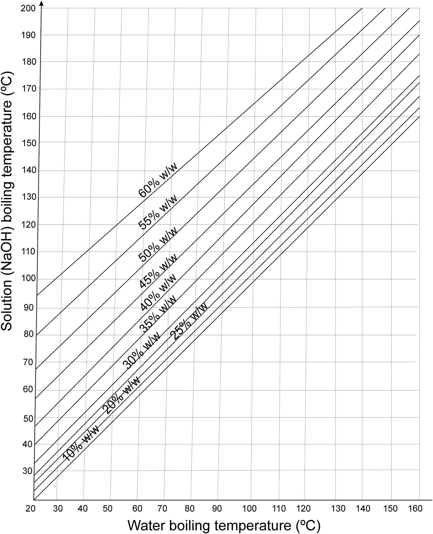
If solution heat is not negligible, then enthalpy is not a function of temperature alone, but also of the concentration. For NaCl solutions, the increase in the boiling point of the solutions is presented in the Dühring diagram in Fig. 4.5. For NaOH solutions, Fig. 4.7 shows the correspondent diagram. Furthermore, the enthalpy of the NaOH liquid solutions can be determined using Fig. 4.8.

For an useful temperature interval, the driving force for the heat transfer in the evaporator is the temperature gradient between chambers. In the evaporation chamber, the temperature is that of the water boiling point plus the ebullioscopic increment due to the solutes dissolved. In the condensation chamber, there is saturated steam that condenses. Thus, the driving force is given by:

$\mathrm{\Delta }{T}_{\mathrm{useful}}=T_{\mathrm{cond}}-T_{\mathrm{eb}}-\mathrm{\Delta }e$ (4.7)

(4.7)

The design equation for the evaporator is as follows:

$Q=U·A·\mathrm{\Delta }T$ (4.8)

(4.8)

where U is the global heat transfer coefficient, A, the contact area, and ΔT is the temperature gradient. See example 4.2 for the design of a single-effect evaporator.

Example 4.2

A simple evaporator processes 10,000 kg/h of a NaOH solution, 20% by weight. A final concentration of 50% is required. The available heating utility is saturated steam at 5 atm, and the evaporation chamber operates at 150 mmHg. The global heat transfer coefficient is 2500 kcal/m²h°C. The feed to the system is at 20°C. Compute:

a. The flowrate of heating utility.

b. The area of the evaporator.

c. The steam economy of the system.

Solution

a. Fig. 4E2.1 shows a scheme of the operation.

We formulate a mass balance to the solids to determine the concentrated liquid flow rate, L, and the evaporated water, E:

$\begin{array}{l}F·x_{\mathrm{f}}=L·x_{\mathrm{L}}\hfill \\ L=\frac{10000\frac{\mathrm{kg}}{\mathrm{h}}·0.2}{0.5}=4000\frac{\mathrm{kg}}{\mathrm{h}}\hfill \end{array}$

$\begin{array}{l}F=L+E\hfill \\ E=6000\frac{\mathrm{kg}}{\mathrm{h}}\hfill \end{array}$

Next, an energy balance to the system is formulated as follows:

$W·H_{\mathrm{w}}+F·h_{\mathrm{f}}=W·h_{\mathrm{w}}+E·H_{\mathrm{e}}+L·h_{\mathrm{L}}$

The enthalpies of the liquid streams—the feed and the concentrated liquid, h_f and h_l, respectively—are shown in Fig. 4.8 as a function of their temperature and composition. H_e is the superheated steam enthalpy, which is a function of the ebullioscopic increment in the boiling point. Fig. 4.7 can be used to determine the difference in the boiling point of the product liquid phase, L, taking into account that at 150 mmHg the boiling point should be 60°C. The properties of the saturated steam can be taken from tables. Thus, the energy balance yields:

$\begin{array}{l}W·{\lambda }_{\mathrm{w},5\mathrm{atm}}+F·h_{\mathrm{f}}(20°\mathrm{C},20\%)=\hfill \\ E·H_{\mathrm{e}}(H_{\mathrm{vsat},{\mathrm{Teb}}_{150\mathrm{mmHg}}}+0.46·\mathrm{\Delta }{e}_{50\%})\hfill \\ +L·h_{\mathrm{L}}(Te{b}_{150\mathrm{mmHg}}+\mathrm{\Delta }{e}_{50\%},50\%)\hfill \\ W·503\text{kcal}/\text{kg}+10000·14.2\text{kcal}/\text{kg}=6000·643.4\text{kcal}/\text{kg}+4000·136\text{kcal}/\text{kg}\hfill \\ W=8400\text{kg}/h\hfill \end{array}$

See Table 4E2.1 for the results.

Table 4E2.1

Results

Heating Utility
Pressure (mmHg)	3800
T (°C)	152.315955
λ (kcal/kg)	503.115296

Solution
Pressure (mmHg)	F	L	E (vapor rec)
Tini (°C)	20	104.7	104.7
C (%w/w)	20	50
Hdis (kcal/kg)	14.22852	136.374159	643.6
	P (mmHg)	T (boiling, water)	C (%)	T+Δe
Outlet	150	60.08°C	50	104.7

b. Thus, the heat transfer area is determined as follows:

$Q=W·{\lambda }_{\mathrm{w}}=U·A·\mathrm{\Delta }{T}_{\mathrm{util}}\Rightarrow A=\frac{W·{\lambda }_{\mathrm{w}}}{U·\mathrm{\Delta }{T}_{\mathrm{util}}}=\frac{4.23·{10}^6\text{kcal}/h}{2500\frac{\mathrm{kcal}}{{\mathrm{m}}^{2}h°C}(152.3-104.7)°\mathrm{C}}=36{\mathrm{m}}^2$

c. The vapor economy, Ec, of the process is given by the following equation:

$Ec=\frac{E}{W}=\frac{6000}{8400}=0.71$

Multieffect Evaporators

This is the typical configuration for the operation of evaporators. The vapor phase generated in the first effect is used to evaporate water from the solution fed to the second effect. In order for the system to operate, as we go along the evaporator train, the evaporation chamber pressure decreases to maintain a driving force between chambers. There are a number of alternative operating conditions, depending on the direction of the flows and the feed to the evaporators.

There are four types of feed systems:

a. Direct Feed. The direction of the vapor and that of the liquid to be concentrated is the same along the evaporator train. Fig. 4.4 is an example of this operation. The pressure at the evaporator chamber decreases in the flow’s direction. The mass and energy balances to this system are given by the following system of equations:

$\begin{array}{l}F-L_n=\sum _n{E}_i\hfill \\ W·{\lambda }_{\mathrm{w}}+F·h_{\mathrm{f}}=E_1·H_{\mathrm{e1}}+L_1·h_{\mathrm{L1}}\hfill \\ E_1·({\lambda }_{\mathrm{e}1}+0.46\mathrm{\Delta }{e}_1)+L_1·h_{\mathrm{L1}}=E_2·H_{\mathrm{e2}}+L_2·h_{\mathrm{L2}}\hfill \\ E_2·({\lambda }_{\mathrm{e2}}+0.46\mathrm{\Delta }{e}_2)+L_2·h_{\mathrm{L}2}=E_3·H_{\mathrm{e}3}+L_3·h_{\mathrm{L}3}\hfill \\ H_{\mathrm{e}i}=H_{\text{sat},\text{boilingwater}}+c_p\mathrm{\Delta }{e}_i\hfill \\ h_{\mathrm{L},i}=h_{\mathrm{dis}}({\%}_i,T_{b,\text{water}}+\mathrm{\Delta }{e}_i)\hfill \end{array}$ (4.9)

(4.9)

b. Countercurrent feed. The direction of the heating vapor and that of the liquid to be concentrated are opposite. The liquid is fed to the last effect. See Fig. 4.9A.

c. Mixed feed. Part of the system is fed following a direct scheme and the rest as countercurrent. See Fig. 4.9B for a scheme.

d. Feed in parallel. The liquid to be concentrated is simultaneously fed to all effects.

There is a useful temperature gradient in a multieffect system. The actual driving force is computed as the difference between the condensing temperature at the steam chamber and the boiling point of water at the last of the effects. From this difference we have to deduct the ebullioscopic increments in the various evaporators of the system. Thus, the useful gradient of temperature decreases with the number of effects, reducing the number of effects that can be used. The advantage of the multieffect evaporator system is a lower energy consumption, while its individual efficiency is lower than a single-effect system.

$\mathrm{\Delta }{T}_{\mathrm{useful}}=T_{\mathrm{o}}-T_n-\sum \mathrm{\Delta }{e}_i$ (4.10)

(4.10)

There are two approaches that can be used for the design of a multieffect evaporator system. There is the computational-based one, depicted in Martín (2014), where advanced modeling and simulation techniques were required to include the thermodynamic models of the mixtures; or the traditional iterative approach, based on the schemes in Figs. 4.7 and 4.8. For the sake of argument, here we only discuss the second one and leave it to the reader to investigate the modeling-based approach. The iterative approach consists of six stages:

1. Perform a mass balance to the system to compute the total vapor generated:

$F=L+E$ (4.11)

(4.11)

2. Assume that all the effects are equal, including their size and the energy exchanged. Thus we distribute the useful driving force among the effects inversely proportional to the global heat transfer coefficient.

3. Formulate the energy balances to all effects.

4. Solve the system of equations evaluating the evaporated flowrate at each one of them.

5. Compute the contact area of each effect. If they are the same, we are done. If not, we must proceed to stage 6.

6. Redistribute the driving force as follows:

$\mathrm{\Delta }\prime T_1=\mathrm{\Delta }T\frac{q_1/U_1}{\sum q/U};\mathrm{\Delta }\prime T_2=\mathrm{\Delta }T\frac{q_2/U_2}{\sum q/U}$ (4.12)

(4.12)

Example 4.3

In the production of NaOH from Na₂CO₃, a 12% w/w solution is obtained. Its concentration for further use must be 38%. Thus a three-effect evaporation system is employed. The initial feed consists of a flowrate of 13,500 kg/h at 25°C, and it is fed to the first effect in direct-feed operating mode. Saturated steam at 4 kg/cm² is available as heating utility. It leaves the first effect as saturated liquid. The absolute pressure at the evaporation chamber in the first effect is 0.1 kg/cm² and the global heat transfer coefficients are 1460, 1250, and 1050 kcal/m² h°C, respectively.

Assuming that all the effects are similar, and that we have as fuel a gas mixture that is 90% methane and 10% nitrogen (by volume) at 25°C and 1 atm, determine the flowrate of fuel (m³/h) required for the operation of the evaporation system if the combustion efficiency is 80%.

Solution

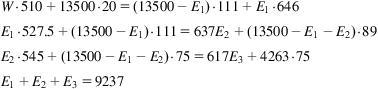
Fig. 4E3.1 shows the scheme of the process for concentrating NaOH using a three-effect evaporator system. We follow the method proposed above. Using a mass balance we compute the product, L=4263 kg/h, and the total vapor, E=9237 kg/h. Assuming that all the effects work similarly, the evaporated water at each effect is E_i=3079 kg. With this and the mass balances to each of the effects:

$L_{i-1}=L_i+E_i$

$L_{i-1}·x_{\mathrm{L}i-1}=L_i·x_{\mathrm{L}i}$

The composition of the liquid flows is as follows:

$x_1=0.155,x_2=0.22,x_3=0.38$

Using Fig. 4.7, the ebullioscopic increments for the three-liquid composition are 3°C, 5°C, and 23°C, respectively. The boiling point at the third effect pressure, 0.1 atm, is 46°C.

Thus, the useful temperature gradient is as follows:

$\mathrm{\Delta }{T}_{\mathrm{useful}}=144-46-3-5-23=67°\mathrm{C}$

Redistributing the temperature gradient inversely proportional to U we have the following:

$\mathrm{\Delta }{T}_1=18.7°\mathrm{C},\mathrm{\Delta }{T}_2=21.8°\mathrm{C},\mathrm{\Delta }{T}_3=25.97°\mathrm{C}$

We now build Table 4E3.1. Starting from the highest temperature, that of the saturated steam, we go down bit-by-bit, computing the temperatures at the different effects and their boiling temperatures. Note that most of the energy transfer from the supersaturated vapor to the next effect takes place at the boiling point, and thus that temperature is used to compute the ΔΤ for area calculation purposes. With these values in the second column of Table 4E3.1, and the composition of the liquid phase, we compute the enthalpies. For instance, the latent heats are evaluated at the boiling temperatures (Tb), while the enthalpies of the vapor phases are those of the superheated vapor at the chamber temperature (T).

Table 4E3.1

Enthalpy Data for Example 4.3

	T (°C)	λ(kcal/kg)	Reheat	Total(kcal/kg)	Hdis(kcal/kg)	Hvap(kcal/kg)
Vapor 1	144	510	0	510
ΔT1	18.7
TI	125.2				111
Δe1	3
Tb I	122.2	526	1.5	527.5		646
ΔT2	21.8
T II	100.4				89
Δe2	5
Tb II	95.4	543	2.5	545		637
ΔT3	26
T III	69.4	559			75
Δe3	23
Tb III	46.4	571	11.5	583		617

We now can solve the energy balances to each of the effects to compute W, E₁, E₂, and E₃:

$\begin{array}{l}W·510+13500·20=(13500-E_1)·111+E_1·646\hfill \\ E_1·527.5+(13500-E_1)·111=637E_2+(13500-E_1-E_2)·89\hfill \\ E_2·545+(13500-E_1-E_2)·75=617E_3+4263·75\hfill \\ E_1+E_2+E_3=9237\hfill \end{array}$

Thus we obtain:

$W=5100\mathrm{kg}/h;E_1=2566\mathrm{kg}/h;E_2=2921\mathrm{kg}/h;E_3=3751\mathrm{kg}/\mathrm{h}$

We see that the evaporated flowrates are not the same, and neither are the areas. Thus, we redistribute the temperatures again and go back. Table 4E3.2 presents the results of the operation of the system.

Table 4E3.2

Results for Example 4.3

The energy to be provided:

$W{\mathrm{\lambda }}_{\mathrm{w}}=2,683,000\text{kcal}/h.$

This energy is obtained from natural gas. The stoichiometry is as follows:

${\mathrm{CH}}_4+0.11{\mathrm{N}}_2+2({\mathrm{O}}_2+3.76{\mathrm{N}}_2)\to {\mathrm{CO}}_2+2{\mathrm{H}}_2\mathrm{O}+(0.11+1.5·3.76){\mathrm{N}}_2$

Assuming liquid water, the energy produced in the combustion of the gas is computed as follows:

$\mathrm{\Delta }{H}_{\mathrm{r}}={\sum \mathrm{\Delta }{H}_{\mathrm{f}}|}_{\mathrm{p}}-{\sum \mathrm{\Delta }{H}_{\mathrm{f}}|}_{\mathrm{r}}=-94.052+2(-57.8)+17.889=-191.76\text{kcal}/\text{mol}$

Assuming an efficiency of 80%, the flowrate of gas required is given by the following expression:

$n=\frac{2.68·{10}^6}{0.8·191.76}=17500\frac{{\mathrm{mol}}_{{\mathrm{CH}}_4}}{\mathrm{h}}\equiv 19700\frac{{\mathrm{mol}}_{\mathrm{gas}}}{\mathrm{h}}\equiv 480{\mathrm{Nm}}^3/h$

Sometimes in the evaporation the liquid is saturated and crystals are formed. Therefore, apart from evaporators, the units act as crystallizers. Crystallization is a separation based on the formation of a pure solid. In the case of penicillin, it is from a solution and it occurs by supersaturation. In this way the solubility of the solid in the solution is overcome. There is a phase equilibrium between the solid and liquid phases. Three regions are found: undersaturated, metastable, and labile solutions. Only in this last region are new crystals formed spontaneously, by nucleation. In the metastable region crystals can grow, while in the undersaturated region any crystals dissolve. Supersaturation can be accomplished by cooling/heating, via evaporation of the solvent at constant temperature, or by using a mixed process, adiabatic evaporation. Alternatively, supersaturation can be achieved via precipitation using a chemical or salting-out by adding a second solvent.

The analysis of crystallization processes is carried out using population balances, accounting for the generation, growth, and death of the crystals. This state can be modeled using a mass transport balance of the species from the bulk to the solid. Assuming that the volume and the surface area are proportional to a characteristic length, we obtain:

${\rho }_{\mathrm{c}}\alpha L^2\frac{dL}{dt}=\frac{d{\rho }_{\mathrm{c}}V}{dt}=\frac{dM}{dt}=A·N_{\mathrm{A}}=A·K_{\mathrm{C}}·\mathrm{\Delta }{C}^n=\beta L^2·K_{\mathrm{C}}·\mathrm{\Delta }{C}^n=G$ (4.13)

(4.13)

This holds if there is uniform supersaturation of the media and there is no crystal breakage (death); thus the growth rate is independent of the size, ie, McCabe’s ΔL law. It is widely used in crystallization modeling. By performing a population balance to a perfectly mixed tank, the concentration of particles of size L, assuming mixed product removal, n_o=n, no seeding and no breakage of crystals, and that McCabe’s ΔL law holds:

$\frac{\partial Vn}{\partial t}=\frac{\partial n}{\partial t}+n\frac{\partial \ln V}{\partial t}=\frac{n_i}{{\tau }_i}-\frac{n_{\mathrm{o}}}{{\tau }_{\mathrm{o}}}-\frac{\partial Gn}{\partial L}+B-D\Rightarrow \frac{dn}{n}=-\frac{dL}{G\tau }\to n=n_{\mathrm{o}}{e}^{-L/(G\tau )}$ (4.14)

(4.14)

where G is the growth rate and τ the residence time (V/Q). The design of these crystallizers is carried out by solving:

• Mass balance to the solute.

• Global mass balance. Accounting for evaporation rate.

• Residence time. Compute the size of the tank.

• Nucleation rate.

• Growth rate.

• Population balance. Compute total mass of crystals, M=6αρ_pn_o(Gτ)⁴.

• Modal size of the crystal. The dominant crystal size, L_D, is 3 Gτ.

Example 4.4

A three-effect evaporator system (see Fig. 4E4.1) is fed with 30 t of brine, 15% by weight of NaCl. From the first effect, 12 t of water are evaporated. From the second, 8 t are evaporated, and 6 t from the last one. The salt crystals are recovered in a conic hopper. During this operation, the level inside the evaporator decreased. The cross-sectional area of the evaporators is 15 m³/m. Table 4E4.1 shows the operating data of the system. Compute the mass of NaCl obtained at each evaporator and the concentrated solution obtained from evaporator III, if its final composition has to be 35%.

Table 4E4.1

Operating Parameters of the Multieffect Evaporator System

	Evaporator
	I	II	III
Feed (t)	30
Feed composition	0.15
Level decrease (m)	0.04	0.05	0.03
Evaporated water (t)	12	8	6
Solubility of NaCl % weight	30	32	35
Concentrated compositions % weight	18	22	35
Density (t/m3)	1.140	1.145	1.150

Solution

We formulate the mass balances to the solid (a), the liquid (b), the brine (c), and the crystals (d), for each effect as follows:

$\begin{array}{ll}F·x_{\mathrm{f}}+B_{C,I}=C_{\mathrm{I}}+L_{\mathrm{I}}{x}_{s,I}\hfill & (\mathrm{a})\hfill \\ F·(1-x_{\mathrm{f}})+B_{\text{Wa},I}={\mathrm{Vap}}_{\mathrm{I}}+L_{\mathrm{I}}(1-x_{s,I})\hfill & (\mathrm{b})\hfill \\ B_{C,I}+B_{\text{Wa},I}=h_{\mathrm{I}}·A·{\rho }_{\mathrm{Brine}}\hfill & (\mathrm{c})\hfill \\ B_{C,I}={\mathrm{sol}}_{\mathrm{I}}·(B_{C,I}+B_{\text{Wa},I})\hfill & (\mathrm{d})\hfill \end{array}$

where B_C is the solids in the brine and B_Wa is the water in the brine; C is the crystals generated; F, L, and Vap are the flows of liquid fed, concentrated solution, and vapor; x is the salt concentration; h is the level of brine descended; A is the cross-sectional area; sol is the solubility of the salt in the operating conditions of the evaporators; and ρ is the brine density.

We do the same for effects II and III:

$\begin{array}{l}{L}_{\mathrm{I}}·x_{s,I}+B_{C,\text{II}}=C_{\mathrm{II}}+L_{\mathrm{II}}{x}_{s,\text{II}}\hfill \\ L_{\mathrm{I}}·(1-x_{s,I})+B_{\text{Wa},\text{II}}={\mathrm{Vap}}_{\mathrm{II}}+L_{\mathrm{II}}(1-x_{s,\text{II}})\hfill \\ B_{C,\text{II}}+B_{\text{Wa},\text{II}}=h_{\mathrm{II}}·A·{\rho }_{\mathrm{Brine}}\hfill \\ B_{C,\text{II}}={\mathrm{sol}}_{\mathrm{II}}·(B_{C,\text{II}}+B_{\text{Wa},\text{II}})\hfill \end{array}$

$\begin{array}{l}{L}_{\mathrm{II}}{x}_{s,\text{II}}+B_{C,\text{III}}=C_{\mathrm{III}}+L_{\mathrm{III}}{x}_{s,\text{III}}\hfill \\ L_{\mathrm{II}}(1-x_{s,\text{II}})+B_{\text{Wa},\text{III}}={\mathrm{Vap}}_{\mathrm{III}}+L_{\mathrm{III}}(1-x_{s,\text{III}})\hfill \\ B_{C,\text{III}}+B_{\text{Wa},\text{III}}=h_{\mathrm{III}}·A·{\rho }_{\mathrm{Brine}}\hfill \\ B_{C,\text{III}}={\mathrm{sol}}_{\mathrm{III}}·(B_{C,\text{III}}+B_{\text{Wa},\text{III}})\hfill \end{array}$

We see that the variables that we have at each effect are as follows:

$B_{\mathrm{C},i},C_i,B_{\mathrm{Wa},i},L_i$

We can actually solve each evaporator one after the other, or the three simultaneously. See Table 4E4.2 for the results.

Table 4E4.2

Operating Parameters of the Multieffect Evaporator System

I		II		III
F=	30	LI=	20.06	LII=	11.59
xf=	0.15	xs,I=	0.18	xs,II=	0.22
BC,I=	0.2052	BC,II=	0.27	BC,III=	0.1811
Ba1=	0.4788	Ba2=	0.5839	Ba3=	0.3364
CI=	1.43	CII=	1.06	CIII=	0.73
LI=	17.07	LII=	11.59	LIII=	5.19
xs,I=	0.18	xs,II=	0.22	xs,III=	0.35
Vap1=	12	Vap2=	8	Vap3=	6
hI (m)	0.04	hII (m)	0.05	hIII (m)	0.03
ρ1 (t/m3)	1.14	ρ 2 (t/m3)	1.145	ρ 3 (t/m3)	1.15
Area (m3/m)	15	Area (m3/m)	15	Area (m3/m)	15
Sol	0.3	Sol	0.32	Sol	0.35

Therefore we obtain 3.23 t of crystals and a concentrated solution of 5.19 t of water 35% of NaCl.

Vapor recompression. This modification involves the compression of the vapor generated in the evaporation. The compressed vapor is used as heating utility.

Solar evaporators: The operation of this units is based on gas–liquid separation with no boiling. The system consists of pools of water covered with plastic or glass. The water evaporates to a dry air so that the distance to saturation is the driving force for the process. Solar energy is the source for heating up the water, and the evaporated water condenses on the surface of the films or the glasses. Proper design allows collecting the condensed drops. Currently, work is being carried out to overcome losses in efficiency due to the reflection of the transparent film, the drops on the surface, the water surfaces and that of the ground, and the radiation from the water bulk. Fig. 4.10 shows schemes of several designs.

4.2.2.1.2 Freezing

Water desalination via freezing is based on the generation of a liquid–solid interphase that is permeable to water only. The solid is obtained by freezing a layer of water. The ice crystals remain in the water and must be recovered. The drawbacks of this technology are that on the one hand there is salt trapped within the crystal, and on the other hand the salt also remains on the crystal surface and freshwater is needed for washing.

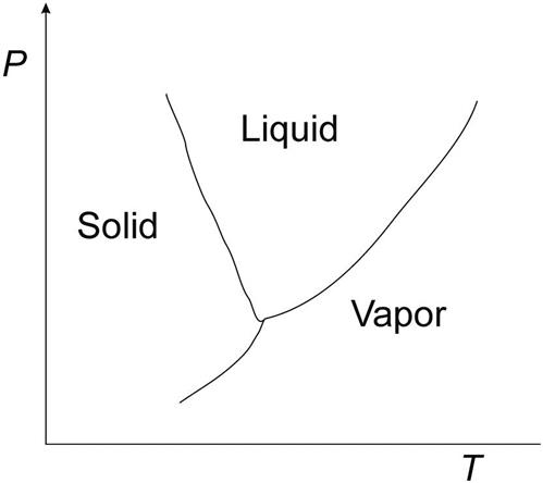
Taking a look at Fig. 4.11, the water phase diagram, we realize that by reducing the pressure and removing the heat, it is possible to freeze water.

Furthermore, by compressing a vapor phase at constant temperature, it is also possible to obtain crystals. There are two main methods for doing this:

a. Water expansion. Vacuum freezing. Seawater is frozen at −4°C and 3 mmHg. In the evaporation it cools down, generating the ice crystals. To maintain the vacuum, the vapor generated in the expansion must be removed either using a compressor or by absorbing it into a hydroscopic solution. The large amount of vapor generated is a technical challenge.

b. Use of a refrigerant. We use a refrigerant whose vapor pressure is above that of water and that is not miscible with it; for instance, butane. When it is expanded, the cooling process freezes the water, generating ice crystals that are easily separated. Fig. 4.12 shows the cycle. The ice is melted, cooling down the refrigerant after recompression, and the water is either used to wash the crystals or as product.

4.2.2.1.3 Hydrate production

This method consists of the production of hydrates by combining water and halogenated organic chemicals. These species can be separated from the brine and later decomposed to recycle the organic species.

4.2.2.1.4 Extraction using solvents

An organic solvent, immiscible with the brine and partially miscible with fresh water, is used for extraction.

4.2.2.1.5 Reverse osmosis

Reverse osmosis is the process by which a semipermeable membrane is used to separate or purify a liquid by permeation King (1980). The concentrated solution cannot permeate it. This technology allows the highest level of separation between salts and water, and it is based on the natural operation of living organisms. The osmosis process was the one observed. When two solutions of different concentration are put into contact across a membrane, water flows from the less concentrated chamber to dilute the second solution (Fig. 4.13A). This flow only stops when the pressure at both sides reaches an equilibrium (Fig. 4.13B). This phenomenon is known as osmosis. Osmotic pressure is so-called because the increase in the volume, and thus in the liquid height, generates a difference in hydrostatic pressure.

The osmotic pressure for two components (the solute and the liquid) in the equilibrium across a membrane can be estimated as follows:

$\mathrm{\Delta }{P}_{\mathrm{eq}}=-(RT/VA)\ln ßA$ (4.15)

(4.15)

For a dilute solution:

$\ln ßA=-(n_{\mathrm{B}}/n_{\mathrm{A}})$ (4.16)

(4.16)

where n_A is the number of moles of solvent and n_B is the number of moles of solute. Upon observing this phenomenon, the idea of reversing it came to mind. If a pressure equal to or above the osmotic pressure is applied to the side of the concentrated solution (Fig. 4.13C), the solvent is forced across the membrane, ie, reverse osmosis.

Separation factors

In reverse osmosis there are two driving forces. On the one hand, there is the pressure difference. On the other hand, there is the gradient in solute concentration. Thus, the flow of each of the species, the solvent (A) and the solute (B), can be calculated as follows:

$N_{\mathrm{A}}=K_{\mathrm{A}}(\mathrm{\Delta }P-\mathrm{\Delta }\pi )$ (4.17)

(4.17)

$N_{\mathrm{B}}=K_{\mathrm{B}}(C_{\mathrm{B}1}-C_{\mathrm{B}2})$ (4.18)

(4.18)

where N_A and N_B are the flows of both components across the membrane (A represents water and B represents the salt).

ΔP: Pressure difference across the membrane.

Δπ: Osmotic pressure difference across the membrane.

C_B1, C_B2: Salt concentration at both sides of the membrane.

K_A, K_B: Empiric constants as a function of the membrane and the salts.

In the equilibrium the ratio $\frac{C_{\mathrm{A}2}}{C_{\mathrm{B}2}}$ should be proportional to $\frac{N_{\mathrm{A}}}{N_{\mathrm{B}}}$. Thus dividing both expressions we have:

$\frac{C_{\mathrm{A}2}}{C_{\mathrm{B}2}}=\frac{N_{\mathrm{A}}}{N_{\mathrm{B}}}=\frac{K_{\mathrm{A}}(\mathrm{\Delta }P-\mathrm{\Delta }\pi )}{K_{\mathrm{B}}(C_{\mathrm{B}1}-C_{\mathrm{B}2})}$ (4.19)

(4.19)

Assuming that the membrane does not allow the salt to cross, the following relationships hold:

$C_{\mathrm{B}2}\to 0\text{and}{C}_{\mathrm{B}2}\ll C_{\mathrm{B}1}$

Thus, Eq. (4.19) becomes:

${\alpha }_{\mathrm{A}-\mathrm{B}}=\frac{C_{\mathrm{A}2}}{C_{\mathrm{B}2}}=\frac{N_{\mathrm{A}}}{N_{\mathrm{B}}}=\frac{K_{\mathrm{A}}(\mathrm{\Delta }P-\mathrm{\Delta }\pi )}{K_{\mathrm{B}}(C_{\mathrm{B}1})}$ (4.20)

(4.20)

Rearranging the variables we have Eq. (4.21):

$\frac{C_{\mathrm{A}2}{C}_{\mathrm{B}1}}{C_{\mathrm{B}2}}=\frac{K_{\mathrm{A}}(\mathrm{\Delta }P-\mathrm{\Delta }\pi )}{K_{\mathrm{B}}}$ (4.21)

(4.21)

Thus, the separation factor f becomes:

$\frac{C_{\mathrm{A}2}{C}_{\mathrm{B}1}}{C{}_{\mathrm{A}1}C_{\mathrm{B}2}}=\frac{{(C_{\mathrm{B}}/C_{\mathrm{A}})}_1}{{(C_{\mathrm{B}}/C_{\mathrm{A}})}_2}=\frac{K_{\mathrm{A}}(\mathrm{\Delta }P-\mathrm{\Delta }\pi )}{K_{\mathrm{B}}{C}_{\mathrm{A}1}}=f$ (4.22)

(4.22)

where 1/C_A1 is equal to 1/ρ_Α, water density, which is constant.

Membrane characteristics

Membranes are the key element in reverse osmosis. They allow the flow of solvents and reject salts. Their filtration capacity depends on the chemical composition of the fluid to be processed and the interaction with the solute. Furthermore, the material behaves differently when the process takes place at different temperatures and pressures. Finally, the amount of solids to be removed also affects the purification process. Therefore, there are some general characteristics that a material must have in order to be used as a membrane:

• It must be highly permeability to freshwater and must reject salts.

• It should be resistant to chemicals.

• It must have high stability over a wide range of pH.

• It must have high resistance to pressure.

• It must have high endurance.

Types of membranes by materials

Inorganic membranes are made of ceramic materials that present high chemical stability. However, they are fragile and expensive, and therefore their use is only recommended for high-temperature processing.

There are two types of organic membranes that can be distinguished as a function of their chemical composition: cellulosic membranes and aromatic polyamide membranes.

Cellulosic membranes are based on cellulose acetate, and are appropriate for processing large flow rates. They can be arranged as pipes, as plane sheets in spiral, or as hollow fibers.

Aromatic polyamide membranes typically process smaller flowrates, but their specific surface is 15 times larger than that provided by their cellulosic counterparts. Furthermore, they are more stable against chemical and biological agents.

Membrane configurations

There are four membrane configurations: modules with plane membranes, modules with tubular membranes, modules with spiral membranes, and modules of hollow fiber.

Modules with plane membranes: This configuration is no longer in use due to its high price. It typically provides 50–100 m²/m³ and pressure drops of 3–6 kg/cm². A preliminary filtration is required to remove suspended solids, and the membrane must be supported. The regeneration requires high-pressure water or the use of chemicals. The product purity is high.

Modules with tubular membranes: These membranes are allocated inside porous tubes that provide support. The surface area that they provide is 50–70 m²/m³. Pressure drops of around 2–3 kg/cm² are also typical. These modules do not require previous filtration, and they can be regenerated chemically, mechanically, or using pressurized water. The cost is also typically high. Fig. 4.14 shows the packing of these membranes inside the tube.

Modules with spiral membranes (axial or radial flow): These modules are built by surrounding a permeable tube with the membranes separated by porous material. They allow good purification, and different structures and materials are employed such as spiral polyamide and spiral cellulose acetate and triacetate. The modules can be standard or for high rejection. In this last case the production capacity is lower in order to increase the purity of the product by rejecting 90–99% of the NaCl. The surface area provided is 600–800 m²/m³ for a pressure drop of 3–6 kg/cm². They require preliminary filtration to remove particles from 10 to 20 μm. Membrane cleaning can be carried out with pressurized water or using chemicals. The cost is lower than the previous configurations, but they need support for the membrane. Fig. 4.15 from AMTA shows the scheme of the configuration, operation, and construction. The feed solution permeates across the layers of membrane material until it reaches the center tube that recovers the permeate. The rest remains in the membrane.

Modules of hollow fiber: The surface area they provide is large, 6000–8000 m²/m³, with a low-pressure drop of 0.2–0.5 kg/cm². These modules require preliminary filtration to remove particles from 5 to 10 μm. They can be cleaned chemically or with pressurized water. The cost is low and they do not need support for the membrane. Fig. 4.16 shows a scheme.

Operation of the membrane modules

Membrane modules can be operated in several configurations: parallel, series, and series production.

In parallel the units operate under the same pressure conditions, producing the same product quality. Typically after the filters, pH is adjusted and chemicals are added. Fig. 4.17 shows the scheme of the installation.

In series the material rejected from the previous unit is processed again to increase production capacity. Fig. 4.18 shows the scheme of the installation.

In series production they are meant to produce high-quality products by processing the permeate of the first system again. The concentrated solution for the second system is recycled to the first one. Fig. 4.19 shows the scheme of the installation.

The modules can operate at three different pressures, depending on the feed to process:

• Low-pressure (10–15 atm) modules: Appropriate for low salinity brines (800–1000 ppm). Ion exchange resins can compete with them.

• Medium-pressure modules (28–35 atm): For salt solutions of 4000–5000 ppm. These were the first on the market.

• High-pressure modules (35–80 atm): Designed to obtain freshwater from seawater since the osmotic pressure is typically from 22 to 27 atm.

To design the membrane modules, we use example 4.5 below. The design equations are given by the flow of solvent and that of salts as presented above in the text.

Example 4.5

Design of reverse osmosis systems. The system is fed with a flow rate of 2.5 kg/s at 8000 kPa. The permeate intended is 1 kg/s at 101 kPa, and the rejected is at a pressure of 7800 kPa.

Data:

Permeability to water: 2.095×10⁻⁶ kg/m² s kPa

Permeability to salt: 3.153×l0⁻⁵ kg/m² s

Initial salinity: 42.000 ppm

Permeate salinity: 145 ppm

Solution

We formulate a global mass balance (M) where f, p, and R refer to feed, permeate, and retentate, respectively. Thus, the flow of retentate is as follows:

$M_{\mathrm{f}}=M_{\mathrm{p}}+M_{\mathrm{R}}$

$2.5=1+M_{\mathrm{R}}\to M_{\mathrm{R}}=1.5\text{kg}/s$

Now, a mass balance to the solute is formulated to compute the concentration:

$M_{\mathrm{f}}·x_{\mathrm{f}}=M_{\mathrm{p}}·x_{\mathrm{p}}+M_{\mathrm{R}}·x_{\mathrm{R}}$

$x_{\mathrm{R}}=69903\mathrm{ppm}$

We assume that all the salts are NaCl. Thus the osmotic pressure of the three solutions is as follows:

${\pi }_{\mathrm{f}}=(x_{\mathrm{f}}/M_{\mathrm{NaCl}})·1000·8.314·298=1779\mathrm{kPa}$

${\pi }_{\mathrm{R}}=2960\mathrm{kPa}$

${\mathrm{\pi }}_{\mathrm{p}}=0.006\mathrm{kPa}$

Bear in mind that in the side of the feed there is a gradient of concentrations since the flow is concentrated. Thus, an average osmotic pressure is calculated as follows:

${{\pi }_{\mathrm{f}}}^{\prime }=0.5({\pi }_{\mathrm{f}}+{\pi }_{\mathrm{R}})=2369\mathrm{kPa}$

And the gradient in osmotic pressure between the permeate and the feed region is as follows:

$\mathrm{\Delta }\pi ={{\pi }_{\mathrm{f}}}^{\prime }-{\pi }_{\mathrm{p}}=2369\mathrm{kPa}$

The pressure gradient applied to the membrane module is as follows, taking into account that at the feed side there is also a pressure gradient:

$\mathrm{\Delta }P=0.5·(8000+7800)-101=7799\mathrm{kPa}$

Thus, the permeate flow is as follows:

$M_{\mathrm{p}}=A·kw·(\mathrm{\Delta }P-\mathrm{\Delta }\pi )$

That allows computation of the area required:

$\begin{array}{l}(1)=A(2.095\times {10}^{-6})(7799-2369)\hfill \\ A=87.9{\mathrm{m}}^2\hfill \end{array}$

We can validate the design by using the salts flow. The mean salinity in the feed side is as follows:

$\begin{array}{ll}x\hfill & =(M_{\mathrm{f}}·x_{\mathrm{f}}+M_{\mathrm{R}}·x_{\mathrm{R}})/(M_{\mathrm{f}}+M_{\mathrm{R}})\\ & =((2.5)(42)+(1.5)(69.903))/(2.5+1.5)\hfill \\ & =52.46\mathrm{kg}/{\mathrm{m}}^3\hfill \end{array}$

Using the design equation for the solids, we have:

$M_{\mathrm{s}}=A·ks·(x-x_{\mathrm{p}})$

We compute the area, and the results are the same as before:

$(1)(0.145)=A(3.153\times {10}^{-5})(52.46-0.145)$

$A=87.9{\mathrm{m}}^2$

Reverse osmosis has a wide range of applications apart from seawater desalination; for instance, the cooling cycles in chemical plants and boiler operation both require pure water. In the operation of these systems, water is evaporated and thus salts are concentrated in the solution. Therefore, salt removal is required at some point.

4.2.2.2 Technologies based on the separation of salts

There are three technologies based on the separation of salts: electrodialysis, ion exchange, and chemical depuration.

4.2.2.2.1 Electrodialysis

This is used to transport salt ions from one solution through ion exchange membranes to another solution under the influence of an applied electric potential difference. The efficiency is computed using the following expression:

$\xi =\frac{ZFQ(C_{\mathrm{inlet}}^{\mathrm{d}}-C_{\mathrm{outlet}}^{\mathrm{d}})}{I}$ (4.23)

(4.23)

where Z is the charge of the ion, F is the Faraday constant, Q is the flow rate of the diluted solution (L/s), C is the concentration of the diluted solution at the inlet and at the outlet (mol/L), and I is the current in amperes.

4.2.2.2.2 Ion exchange

It is used to capture certain ions as a function of their charge. Thus, cationic and anionic resins are available. The exchange between the resin and the ions is as follows for both types of resins, respectively:

$\begin{array}{l}\mathrm{Cationic}\mathrm{R}-\mathrm{H}+{\mathrm{M}}^{+}\leftarrow \to \mathrm{R}-\mathrm{M}+{\mathrm{H}}^{+}\hfill \\ \mathrm{Anionic}\mathrm{R}-\mathrm{OH}+{\mathrm{A}}^{-}\leftarrow \to \mathrm{R}-\mathrm{A}+{\mathrm{OH}}^{-}\hfill \end{array}$

The ion exchange beds cannot handle brines with concentrations above 3500 ppm. Therefore, the applicability is restricted to water cycles in boilers and low salinity aquifers with high content in calcium and magnesium.

4.2.2.2.3 Chemical depuration

In this process, seawater is treated with Cl₂ and CuSO₄ to precipitate the organic matter. Next, CaO and CaCO₃ are added to remove ions such as Cl⁻, SO₄²⁻, Mg²⁺, and Ca²⁺ by precipitation. The water is next treated with NH₄HCO₃ to precipitate NaCl. Finally, active carbon allows one to achieve water with 200–300 ppm of salts. The bed of active carbon is regenerated using NaOH and HCl. A flowsheet for the process is shown in Fig. 4.20.

4.2.3 Water Electrolysis

Water decomposition leads to the production of hydrogen as the most valuable product. The use of electrolysis has been an alternative for quite some time. It has recently received more attention with the development of renewable technologies to produce power from solar to wind energy. However, the high cost (2.6–4.2 $/kg) makes it not as interesting from an industrial point of view, and thus natural gas steam reforming or hydrocarbon partial oxidation are the most widespread methods, as we will see in Chapter 5, Syngas. In spite of the reduced industrial use, less than 3% of hydrogen is produced using electrolysis; we need to bear in mind that the use of hydrocarbons as a source for hydrogen is not carbon-efficient since they have fixed CO₂ from the atmosphere and only H₂ is taken from them. Furthermore, electrolysis using renewable sources (Davis and Martín, 2014) has lately become an alternative to store solar (photovoltaic or PV solar, concentrated solar power) and wind energy in the form of chemicals (using CO₂ as a source of carbon). Thus, the process is twofold: renewable energy storage, and CO₂ capture and utilization.

Water decomposition into its components requires high energy consumption. Water formation energy, ΔH_f, is 68.3 kcal/mol at 25°C. However, only the fraction corresponding to the Gibbs free energy can be provided as work (ΔG=56.7 kcal/mol at 25°C), and the rest (TΔS) needs to be provided as heat.

$\mathrm{\Delta }{G}_{\mathrm{f}}=\mathrm{\Delta }{H}_{\mathrm{f}}-T\mathrm{\Delta }S$ (4.24)

(4.24)

Solutions with free ions allow current conduction. Thus, the electromotive force that allows conduction is the decomposition potential. The theoretical minimum for the reversible water decomposition can be computed using the Nernst equation as follows:

$\begin{array}{l}\mathrm{\Delta }G=nFE=2\times 96540\times E\hfill \\ \mathrm{\Delta }G\to E=1.23\mathrm{V}\mathrm{at}25°\mathrm{C}\hfill \\ \mathrm{\Delta }H\to E_{\mathrm{eq}}=1.48\mathrm{V}\mathrm{at}25°\mathrm{C}\hfill \end{array}$ (4.25)

(4.25)

The potential difference between both has to be provided by heat. In practice, the actual potential to be applied needs to be from 1.8 to 2.2 V due to the Ohmic loss in the electrolyte, those of the electrodes, and the polarization overpotential. There are a few basic definitions used to characterize the efficiency of the operation of a system.

Unit energy consumption corresponds to the energy consumption to produce a unit of the product. Its inverse is the product obtained per unit of energy, the energy yield of the process.

The energy ratio is the ratio between the theoretical work (Gibbs free energy) and the power used to produce a certain amount of product:

$\eta =\frac{n_{\mathrm{electrons}}·F·V}{E_{\mathrm{e}}}$ (4.26)

(4.26)

Energy efficiency is the ratio between the energy stored in the product, the low heating value, and that consumed to produce it. Commercial plants operate from 50% to 75% energy efficiency.

The current yield computes the ratio between the theoretical power and that used for the production of a certain amount of product:

$\epsilon =\frac{n·F}{I·t}$ (4.27)

(4.27)

where F is equal to 96,485 C/mol (1 F is the charge of a mol of electrons). The units are equivalent to J/V mol or A·s/mol since 1 Coulomb=1 A·s and 1 Volt=Joule per Coulomb.

4.2.3.1 Commercial electrolyzers

There are two distinct designs: those that use electrolyte solutions and those that employ solid polymer electrolytes. The most used are the first class, and they present two configurations: tank-type and press filters.

1. Tank-type electrolyzers are also known as unipolar electrodes. Each cell consists of a cathode and anode and room for the electrolyte. The electrodes may be separated or even isolated by a diaphragm. The electrodes are connected in parallel and the number of cells needed to reach the production capacity represents the electrolytic system. The potential difference is the same for each cell. The H₂ and O₂ are collected through pipes connected to the anodic and cathodic places, respectively. This is the oldest configuration.
Only a few parts are needed to build them, and they are relatively inexpensive. Tank-type electrolyzers optimize a lower thermal efficiency, and they are typically used for their lower power costs. Furthermore, in terms of maintenance, the individual cells can be isolated or replaced independently of the rest of the configuration. They provide low potential difference and high intensity, and the purity of the hydrogen produced is high.

2. Filter press cells, or bipolar electrolyzers, have their electrodes in series so that one face acts as the cathode and the other as the anode, which results in a compact configuration. Between each electrode there is a diaphragm. They are connected to the electrical grid through the terminal electrodes, simplifying the installation, so that the potential difference is the summation of that corresponding to each element. Thus they work with low current intensity and high potential difference.

In both cases, the electrolyte solution flows in order to be cooled down continuously, and is recycled back to the electrolyzer. This stage represents the major water consumption of the plant. Fig. 4.21A shows a scheme for tank-type electrolyzers, and Fig. 4.21B shows an example of a filter press cell.

Water electrolysis using solar or wind energy has focused on the production of hydrogen for the so-called hydrogen economy. Fig. 4.22 shows a flowsheet for that process. It can operate at atmospheric pressure or above (30 atm) at 60–80°C and with an electrolyte solution, KOH 20–40 wt%. Typically, 500 Nm³/h of hydrogen are produced per unit, consuming 0.9 L of water per Nm³ of hydrogen. The power required is 175,000 kJ/kgH₂ (NEL Hydrogen, 2012). Once the water is split, both gas streams must be purified. The oxygen stream contains water that is condensed, and is later compressed and dehydrated using silica gel or a similar adsorbent. For the hydrogen-rich stream, we do not only need to remove the water that saturates the stream, but more importantly, the traces of oxygen. Therefore, a deoxo reactor that uses a small amount of the hydrogen produced converts the traces of oxygen into water. Finally, a dehydration step using adsorbent beds is used before final compression.

Lately, this hydrogen has been used to hydrate CO₂ and to produce chemicals such as methane, methanol, and DME as a way to store energy. Table 4.5 shows the comparison of these processes based on the work by Martín (2016). See Chapter 5, Syngas, for synthesis details.

Table 4.5

Yield to Products and Consumption for CO₂/H₂-Based Processes

Main Product/Other Products and Raw Materials	CH4	CH3OH	DME
CO2 captured (kg/kg)	3.0	1.4	1.9
H2O consumption (kg/kg)	2.8	1.2	1.3
O2 production(kg/kg)	3.3	1.5	2.1

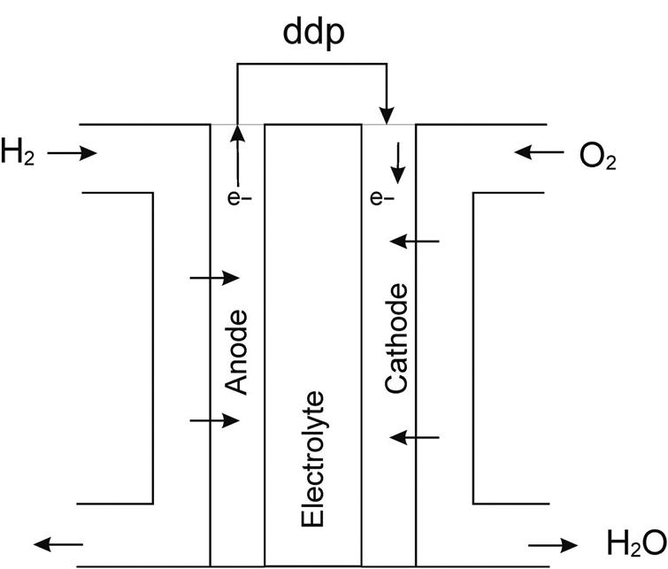
4.2.3.2 Fuel cells

Fuel cells perform the opposite chemical reaction—they transform hydrogen and oxygen into electrical energy. The advantage is the absence of mobile parts, so there is no need for recharge; they have been used in spaceships since the 1960s.

${\mathrm{H}}_2+\frac{1}{2}({\mathrm{O}}_2+3.76{\mathrm{N}}_2)\to {\mathrm{H}}_2\mathrm{O}+Q+\mathrm{Power}$

The process is highly efficient, has no emissions, is quiet, and the byproduct is water. The main drawbacks of the technology are the storage of the hydrogen, the size and weight of the cells, and the high cost of hydrogen. There are a few car makers who have produced models running on hydrogen over the last few decades, but the supply chain of hydrogen is not developed to the point where making the cars is a commercial prospect.

Fig. 4.23 shows an acid fuel cell. The hydrogen is injected into the anode region. It crosses it and reacts with the oxygen at the electrolyte, producing water that exits with the excess of air used. The alkali kind of cell works the opposite, and the water is produced on the hydrogen side.

Example 4.6

We would like to produce 2 kg/s of hydrogen at 30 bar via water electrolysis. We have several sources of renewable energy, including solar, wind, and biomass. The oxygen produced has to be compressed up to 100 bar for its storage. Assume complete water breakup into hydrogen and oxygen, pure hydrogen from the cathode and oxygen from the anode. The compressor’s efficiency is 85%, and the electrolysis occurs at 80°C. The electrolytic cell has an energy ratio of 60%. Assuming that the polytropic coefficient is k=1.4:

a. Compute the energy required for the process.

b. Select the technology using the information in Table 4E6.1.

c. Determine the price of the wind energy for it to be more profitable if the carbon tax for CO₂ emission is 40€/t and the ground is at a cost of 25€/m².

Table 4E6.1

Information on the Technologies

Technology	Cost (€/kW)	CO2 Generated (kg/kW)	Area (m2/kW)
Wind	1300	0.5	0
Solar	1150	1	5
Biomass	1000	0	10

Solution

a. The energy required is that needed to split the water, and for gas compression.
Energy=E+ W(Oxygen line) + W(Hydrogen line)
For the electrolyzer we have the following reaction:

$\begin{array}{ll}{\mathrm{H}}_2\mathrm{O}\to ½{\mathrm{O}}_2+2{\mathrm{H}}^{+}+2{\mathrm{e}}^{-}\hfill & E=-1.23\mathrm{V}\hfill \\ 2{\mathrm{H}}^{+}+2{\mathrm{e}}^{-}\to {\mathrm{H}}_2\hfill & E=0\mathrm{V}\hfill \\ E=0–(-1.23)=1.23\mathrm{V}\hfill & \hfill \end{array}$

$\eta =0.6=\frac{n_{{\mathrm{H}}_2}·e·F·V}{E_{\mathrm{e}}}=\frac{\frac{2000g/s}{2}·2·96500·1.23}{E_{\mathrm{e}}}\Rightarrow E_{\mathrm{e}}=395650\mathrm{kW}$

The energy consumption of the compressors is computed using the next equation. Considering that the compression cannot be made in one stage (due to the pressure difference), but must be made in three stages, the work used is computed as follows:

$W(\text{Comp})=3(F)·\frac{8.314·k·({\mathrm{T}}_{\mathrm{in}}+273.15)}{((\mathrm{MW})·(k-1))}\frac{1}{{\eta }_{\mathrm{s}}}\left({\left({\displaystyle \frac{P_{\mathrm{out}}}{P_{\mathrm{in}}}}\right)}^{\frac{1}{3}\frac{k-1}{k}}-1\right)$