
ΔH: Heat of reaction per mol of N2 (−26,000 kcal/kmol N2)
S2: Cross-sectional area of catalyst zone 0.78 m2
Nitrogen mass balance:

f: Catalyst activity
Pi: Partial pressure of the species
Ki: rate constants,
where

and the pressure drop is given by Ergun’s equation:
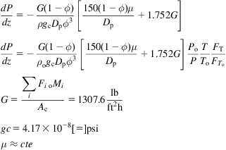
Tf=694K, Tg=694K, P=286 atm, NN2=701.2 kmol/h m2
Feed: 21.75% N2; 62.25% H2; 5% NH3; 4% CH4; 4% Ar.
We model the reactor in gProms. For a further description of the modeling of reactors using gProms, we refer the reader to Martín (2014). We define a model block as:
PARAMETER
S1 as real
S2 as real
eff as real
cooling as real
U as real
Pto as real
ph as real
rhoo as real
Dp as real
visc as real
gc as real
Tgo as real
Cpf as real
Cpg as real
deltaHr as real
R as real
VARIABLE
K1 as notype
K2 as notype
NN2o as concentration
Ni as concentration
NNH3o as concentration
Nto as concentration
Ntotal as concentration
NN2 as concentration
Tf as temperature
Tg as temperature
Presion as Pressure
PN2 as Pressure
PH2 as Pressure
PNH3 as Pressure
ra as notype
G as notype
SET
S1:=10;
S2:=0.78;
eff:=1;
cooling:=26400;
U:=500;
Pto:=286;
ph:=0.45;
rhoo:=0.054;
Dp:=0.015;
visc:=0.090;
gc:=4.17e8;
Tgo:=694;
Cpf :=0.707;
Cpg:=0.719;
deltaHr:=−26000;
R:=1.987;
EQUATION
K1=1.78954e4*exp(−20800/(R*Tg));
K2=2.5714e16*exp(−47400/(R*Tg));
NN2o=0.2125*26400/10.5;
Ni=0.08*26400/10.5;
NNH3o=0.05*26400/10.5;
Nto=4*NN2o+Ni+NNH3o;
Ntotal=Ni+NNH3o+2*NN2o+2*NN2;
PN2=NN2*Presion/Ntotal;
PH2=3*PN2;
PNH3=Presion*((NNH3o+2*(NN2o-NN2))/(Ntotal));
ra=eff*(K1*PN2*PH2^1.5/PNH3-K2*PNH3/(PH2^1.5));
G=0.454*(Ni*16+NN2o*28+3*NN2o*2)/((S2/0.3048^2));
$NN2=−ra;
$Tf=(U*S1*(Tg−Tf)/(cooling*Cpf));
$Tg=−(U*S1*(Tg−Tf)/(cooling*Cpg))+(ra)*(−deltaHr)*S2*eff/(Cpg*cooling);
$Presion=−G*(1−ph)*Pto*Tg*(150*(1−ph)*visc/Dp+1.75*G)*(Nto/(Ni+NNH3o+2*NN2o+2*NN2))/(14.7*rhoo*gc*Dp*ph^3*Tgo*Presion);
PROCESS
Unit R101 as Reactor
INITIAL
WITHIN R101 DO
NN2= 0.2125*26400/10.5;
Tg= 694;
Tf= 694;
Presion=286;
END # Within
SOLUTIONPARAMETERS
ReportingInterval := 0.1 ;
SCHEDULE
CONTINUE FOR 5
The temperature profiles are prsented in (Fig. 5E6.2).
5.4.1.2.4 Production processes
The various processes differ from one to another based on the raw material used, and therefore, the procedure to obtain the syngas and the reactor design.
Kellogg process (medium pressure)
Fig. 5.25 shows a flowsheet for the Kellogg process. In this figure the different sections can easily be recognized. Natural gas is the typical feedstock. After sulfur removal, we have primary and secondary reformers followed by high-temperature and low-temperature sweet shift. Once the syngas is obtained, CO2 is removed. Selexol or MDEA processes are among the selections for the Kellogg design. The traces of CO and CO2 are removed in a methanator. The synthesis occurs in their proprietary converter designs using ruthenium catalyst (Kaap), which has recently substituted the Fe-based ones (after 90 years). The reaction operates at 300°C and 100–130 atm. Next, ammonia is separated. There are some rules that determine the type of separation, condensation, or absorption, depending on the operating conditions. Condensation is recommended above 100 atm in spite of the high fix costs. Absorption typically follows Raoults’ Law (see Chapter 2: Chemical processes).

Haber–Bosch process (medium pressure)
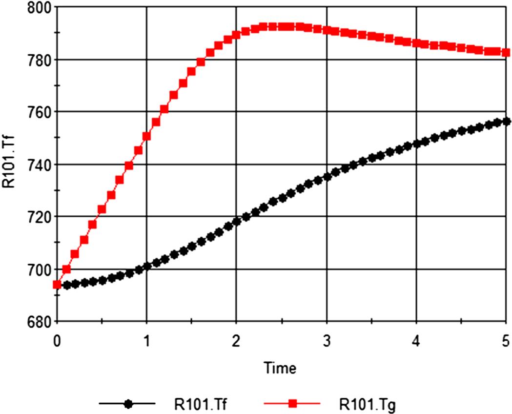
This is one of the most extended processes for the production of ammonia. There are versions that use natural gas, but coal was commonly the raw material. Fig. 5.26 shows the scheme of the process. The syngas is produced using steam, air, and coke. There are a few preparation stages including the scrubber, WGSR, and CO2 capture. The converter operates at 200–350 atm and 550°C. The ammonia concentration in the outlet stream from the converter is from 13% to 15%, and the ratio between the recycle and the feed is 6–7 to 1. The converter is 12 m tall, with an inner diameter of 0.8 m. The wall is 0.16 m thick and uses 6 t of double-promoted iron catalyst (see Fig. 5.27). The purge is around 5%. The ammonia is absorbed in water that is distilled to recover the ammonia (Lloyd, 2011).


Claude’s process (high pressure)
George Claude’s process is characterized by a high operating pressure at the reactor (900–1000 atm), and temperatures in the range of 500–650°C using a promoted iron catalyst. No recirculation is present due to the high conversion achieved—higher than 40%. Since there is no recycle and no purge, the unreacted hydrogen is lost. The catalyst is iron oxidized in magnesia containing 5–10% calcium oxide. Magnesium oxide also dissolves in the mixture. The reactor includes a guard bed to absorb poisons and convert residual CO into methanol. As a result of the pressure, water can be used to condense the produced ammonia out of the product stream. The drawbacks of the process are the compression costs and shorter converter life. Thirty percent of US plants used the Claude process. The reactor is 5 m tall, with an inner diameter of 0.5 m and a wall thickness of 0.3 m. Fig. 5.28 shows a scheme of the original reactor (Lloyd, 2011).

Uhde’s process
The first stages of this process are common to others (see Fig. 5.29). The raw material is typically natural gas that is processed to remove the sulfur compounds. Next, it is mixed with steam to produce the syngas over nickel catalysts. The first reformer operates at 40 atm and 800–850°C to save compression energy later on. This reformer is top-fired, and its tubes are made of a stainless steel alloy for better reliability. In the second reformer, air is added. After gas cooling, the CO is transformed into CO2 using the sweet shift combining HTS and LTS. The process uses ethanolamines for the removal of the CO2, while the traces of CO and CO2 are eliminated via methanation. This process is characterized by the use of two converters with three catalytic beds operating under radial flow conditions; see Fig. 5.30 for a scheme of the reactor. The first reactor consists of an intercooled three bed reactor operating at 110 atm. The second one, operating at 210 atm, is responsible for two thirds of the total ammonia production. The use of this system allows a limited pressure drop. The energy generated is used to produce high-pressure steam. The ammonia is recovered by condensation. The purge is processed to recover the hydrogen, and the rest of the gas is used as flue gas.


Fauser process (old process)
In this process the hydrogen is produced via electrolysis while the nitrogen comes from air fractionation Ernest et al. (1925). Both streams are mixed and compressed up to 200–300 atm after processing to remove oil and oxygen in a deoxo-type reactor.
Water is condensed and removed before feeding the stream to the reactor. The reactor uses iron-promoted catalysts and operates at 500°C, achieving a conversion of 20%. It is 14 m tall with an interdiameter of 0.85 m and a wall thickness of 0.16 m. The ratio between the recycle and the feed is 4.5–5 to 1, and a part of the recycle is purged to avoid build-up. Fig. 5.31 shows a scheme of the reactor, and Fig. 5.32 the process.

Texaco process
The Texaco process is characterized by the technology used in the production of the syngas, the partial oxidation of hydrocarbons. It is called the Texaco syngas generation process (TSGP). Next, WGSR is carried out. Subsequently, the CO2 is captured using the Rectisol process. Fig. 5.33 shows the stages for syngas production in the Texaco process.

Gasification
It is also possible to gasify coal or other carbonous mass for syngas production and later use it to produce ammonia. Gasification was responsible for 90% of the share of ammonia production by the 1940s.
Casale process
The main characteristic of this process, developed by Luigi Casale, is the reactor; a scheme can be seen in Fig. 5.22. It operates at 600 atm and 500°C, and the control of temperature in the reaction is achieved by recycling the gas so that 2–3% ammonia in the feed of the converter is allowed. As a result, the rate of ammonia production is reduced, and with it, the energy generation. The high operating pressures allow the use of cooling water to condense and separate the ammonia. The reactor is typically 10 m tall, with an inner diameter of 0.6 m and a wall thickness of 0.25 m. The ammonia concentration at the reactor exit is around 20% and the ratio between the recycle and the feed is 4–5 to 1 (Vancini, 1961, Lloyd, 2011).
Gas generator/water gas process
This process is characterized by the production of the syngas using the combination of the generator gas and water gas cycles that were presented in the beginning of the chapter. After the gas is generated, sulfur is removed using hydrodesulfurization and later H2S removal stages. Next, WGS is carried out to remove the CO and increase the production of hydrogen. Subsequently, CO2 is captured and the traces of CO are removed using copper. Finally, ammonia is synthesized. Fig. 5.34 shows the flowsheet.

Haldor–Topsoe process
The main feature of this process is that the raw material can be either natural gas or liquid hydrocarbons. After hydrodesulfurization and H2S removal, primary and secondary reforming are performed. Air is injected in the second reformer. Next, HTS and LTS are carried out, and after CO2 removal using Selexol or MDEA, methanation removes the traces of CO and CO2. The main feature of the process is also the use of proprietary radial flow reactors operating at 140 atm. Ammonia can be condensed using water, and 20% of the unconverted gas is lost. Fig. 5.35 shows the flowsheet.

Example 5.7
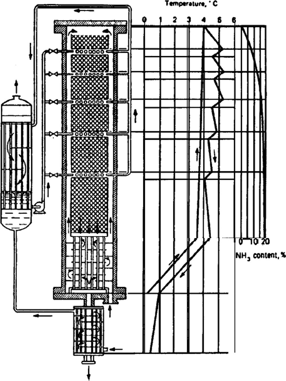
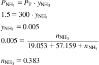
In an ammonia production facility, the converter is fed with a stoichiometric mixture of syngas N2+3H2. The conversion at the reactor is 25% to ammonia. Assume that all the ammonia is separated in a condensation stage. The unconverted gases are recycled to the reactor. The initial feedstock contains 0.2 moles of Ar per 100 mol of mixture. At the entrance of the reaction, a maximum of 5 moles of ammonia per 100 mol of syngas is allowed. Compute the purge.
Solution
The synthesis loop is shown in the figure below. We formulate the mass balance from point 1 onwards, assuming that R is the syngas recycle (Fig. 5E7.1).

For the balance to the converter, the reaction taking place is as follows:
Note that we can consider the syngas a mixture, and that per 4 moles of reactants, 2 moles of ammonia are produced. Using this consideration, only three species are evaluated. Let “Recy” be the recycled syngas (Tables 5E7.1 and 5E7.2):
Table 5E7.1
| In | Reacts | Out | |
| N2+3H2 | 100+Recy | −(100+Recy)·0.25 | (100+Recy)·0.75 |
| NH3 | (2/4) (100+ Recy)·0.25 | (100+Recy)·0.125 | |
| Ar | (100+Recy)·0.05 | (100+Recy)·0.05 |

Table 5E7.2
| In | Ammonia Removal | Out | |
| N2+3H2 | (100+ Recy)·0.75 | (100+Recy)·0.75 | |
| NH3 | (100+ Recy)·0.125 | (100+ Recy)·0.125 | |
| Ar | (100+ Recy)·0.05 | (100+Recy)·0.05 |

The balance to the gas–liquid separator is covered in Table 5E7.2.
For the balance to the divider (the purge) we assume that a fraction of the recycle, α, is purged (Table 5E7.3).
Table 5E7.3
| In | Purge | Recycle | |
| N2+3H2 | (100+Recy)·0.75 | (100+Recy)·0.75·α | (100+Recy)·0.75 (1−α) |
| NH3 | |||
| Ar | (100+Recy)·0.05 | (100+Recy)·0.05·α | (100+Recy)·0.05·(1−α) |

Under steady-state conditions, the Ar fed to the system must be eliminated through the purge. Furthermore, the recycle, assumed to be R, is also a function of the purge. Thus, we have a system of two equations and two variables:
Solving the system we have R=288 and α=0.0103. The compositions of the streams at the four positions along the flowsheet are given in Table 5E7.4.
Example 5.8
The gas exiting the reactor at 400°C and 300 atm contains ammonia in a concentration that corresponds to 30% of the equilibrium value under those conditions. Assume that the pressure does not change across the facility. Assuming humid air calculations with ammonia as the moisture:
a. Compute the composition of the gases at the reactor exit.
b. Determine the gas composition after a cooling stage at 5°C.
c. Compute the gas composition after a second cooling at −25°C
Hint: The equilibrium constant at 400°C and 300 atm is 0.0153.
Solution
As presented in the section describing the equilibrium, the constant is as follows:
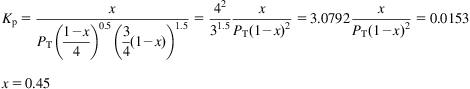
Since only 30% of the conversion at equilibrium is achieved,


the molar gas composition is as follows:

Ammonia vapor pressure at the two temperatures, from Antoine correlation,
is given in Table 5E8.1:
After the condensation, the gas is saturated, and thus:

Thus, the uncondensed moles are computed as follows:

Therefore, 10.6 moles have condensed. After the second condensation, we proceed similarly to compute the ammonia in the gas:
Therefore, 0.91 kmol have been condensed. In total, 11.51 kmol have been recovered out of the 11.8945, around 97% recovery.
Example 5.9
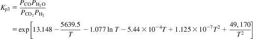
The stream from the reactor consists of 281 kmol of syngas, 9.12 kmol of Ar, and 62 kmol of ammonia. Ammonia is cooled and condenses. Assuming a condensation pressure of 50 atm, compute the temperature of the cooling for recovering 75% of the ammonia produced. Use flash calculations to compute the separation.
Solution
The problem is formulated as a gas–liquid equilibrium using the following nomenclature:
A global balance and a component balance are used to compute the molar fraction of the gas and liquid phases:

Combining the equations:


The vapor compositions are given by the following equations:
The liquid compositions are computed as follows:
where Ki or Kj is equal to Pv/Ptotal. Thus, we fix lj to be 75% of fj for ammonia and solve the system of equations. Alternatively, we can just solve vj=0.25 fj to obtain Kj, and from that the temperature. Table 5E9.1 presents the results. We see that the Ks are within the error of the approximation.

Example 5.10
Compute the liquid flow required to recover 98% of the ammonia content in the product gases of the converters using an absorption column. The total gas flow is 10 kmol/s with 20% ammonia by volume. The stream is at 10 atm and 25°C. The gas flow is 50% of the minimum required. Calculate the number of stages.
Solution
Assume that Raoult’s law holds. Therefore:
The vapor pressure of ammonia is computed using the Antoine correlation as follows:
We formulate a mass balance to the ammonia using as control volume that of the scrubber:
The concentration of ammonia in the liquid is in equilibrium with that of the gas in the inlet, y=0.2.

Lin=7.72 kmol/s. Thus, the flow used is 11.58 kmol/s. yi is the composition of the exiting gas consisting of 8 kmol/s of air and 0.04 kmol of ammonia, yi=0.005.

5.4.2 Fischer–Tropsch Technology for Fuel and Hydrocarbon Production
5.4.2.1 Introduction
FT synthesis dates back to 1902 when Sabatier and Senderens found that the CO could be hydrogenated over catalysts of Co, Fe, and Ni to produce methane. In 1920 Franz Fischer, founding director of the Kaiser Wilhelm Institute of Coal Research in Mülheim an der Ruhr, and his head of department, Dr. Hans Tropsch, presented the formation of hydrocarbons and solid paraffins on Co–Fe catalysts at 250–300°C. FT technology was further developed and became commercial in Germany during the Second World War when their access to crude was denied. Lately, apart from the hydrogenation of CO, the large production of CO2 has made it widely available as a carbon source. Therefore, research has focused on the possibility of using it as a source of methane, methanol, or fuels Eckhard et al. (1998), Weissermel and Arpe (1978).
5.4.2.2 Methanol production
In this section the mechanism of the formation of methanol is depicted. Next, the equilibrium for the production is evaluated, followed by the reactor kinetics, the reactor designs, and a description of the production process.
5.4.2.2.1 Mechanisms
The scheme for the reaction is as follows, where the limiting reactions are marked as “rds”. The mechanism is given by the hydrogenation of CO and CO2 together with the WGS reaction (Vanden Bussche and Froment, 1996):

5.4.2.2.2 Equilibrium
In the reactor, a series of reactions takes place. Only two of the three are linearly independent, and thus the equilibrium model for the reaction can be formulated using the elementary balances to C, O, and H, and the following two equilibrium constants. Note that the WGSR reaction is present. The methanol synthesis is affected by pressure. High pressure drives the reaction to products.

The equilibrium constants are given as follows:
(5.18)
 (5.18)
(5.19)
 (5.19)
The elementary mass balance is given by Eq. (5.20):
(5.20)
 (5.20)
There are two main operating variables that the feed to the reactor must meet for the optimal production of methanol:
• The ratio of hydrogen to CO should be ![]() .
.
• The role of CO2 in the reaction mechanism is not well-known or understood. However, it is considered that the concentration of CO2 should be 2–8%, and the ratio of the syngas components involving CO2 should be the following:
(5.21)
5.4.2.2.3 Kinetics of methanol production
There are a number of models in the literature for the production of methanol from syngas. We consider the work by Vanden Bussche and Froment (1996) as reference. The rates for the production of methanol and the reverse WGS are given by:
(5.22)
 (5.22)
where
(5.23)
 (5.23)
(5.24)
 (5.24)
The equilibrium constants are given by Eq. (5.25),
(5.25)
 (5.25)
and the kinetic constants are of the form given by Eq. (5.26):
(5.26)
 (5.26)
Therefore, the rates are as follows:
(5.27)
 (5.27)
The parameters required are in the following table:
| A | 0.499 | |
| B | 17,197 | |
| A | 6.62×10⁻¹¹ | |
| B | 124,119 | |
| A | 3453.38 | |
| B | – | |
| A | 1.07 | |
| B | 36,696 | |
| A | 1.22×10¹⁰ | |
| B | −94,765 |

Example 5.11
Assume a feed composition of 0.2CO, 5H2, and 0.4CO2, and no inerts. The reactor operates at 493K and 50 atm. Model the reactor.
Solution
Reactor model
PARAMETER
A_rKH2 as Real
A_KH2O as Real
A_quot as Real
A_k5K2K3K4KH2 as Real
A_k1 as Real
B_rKH2 as Real
B_KH2O as Real
B_quot as Real
B_k5K2K3K4KH2 as Real
B_k1 as Real
R as Real
VARIABLE
Temp as Temperature
Press as Pressure
rKH2 as notype
KH2O as notype
quot as notype
k5K2K3K4KH2 as notype
k1 as notype
#% Algebraic equations - equilibrium constants
K as notype
K3 as notype
# Algebraic equations - Partial pressures as ideal gas mixture
P_CO as Pressure
P_H2O as Pressure
P_MeOH as Pressure
P_H2 as Pressure
P_CO2 as Pressure
# Algebraic equations - Reaction rates
r_MeOH as notype
r_RWGS as notype
molCO as molar
molH2O as molar
molMeOH as molar
molH2 as molar
molCO2 as molar
moltotal as molar
SET
A_rKH2:=0.499;
A_KH2O:=6.62e-11;
A_quot:=3453.38;
A_k5K2K3K4KH2:=1.07;
A_k1:=1.22e10;
B_rKH2:=17197;
B_KH2O:=124119;
B_quot:=0;
B_k5K2K3K4KH2:=36696;
B_k1:=-94765;
R:=8.314;
EQUATION
rKH2=A_rKH2*exp(B_rKH2/(R*Temp));
KH2O=A_KH2O*exp(B_KH2O/(R*Temp));
quot=A_quot*exp(B_quot/(R*Temp));
k5K2K3K4KH2=A_k5K2K3K4KH2*exp(B_k5K2K3K4KH2/(R*Temp));
k1=A_k1*exp(B_k1/(R*Temp));
#% Algebraic equations - equilibrium constants
K=10^(3066/(Temp)-10.592);
K3=1/(10^(-2073/(Temp)+2.029));
# Algebraic equations - Partial pressures as ideal gas mixture
moltotal=molCO+molH2O+molMeOH+molH2+molCO2;
P_CO=molCO/moltotal*Press;
P_H2O=molH2O/moltotal*Press;
P_MeOH=molMeOH/moltotal*Press;
P_H2=molH2/moltotal*Press;
P_CO2=molCO2/moltotal*Press;
# Algebraic equations - Reaction rates
r_MeOH=(k5K2K3K4KH2*P_CO2*P_H2*(1-(1/K)*(P_H2O*P_MeOH/(P_H2^3*P_CO2))))/((1+quot*P_H2O/P_H2+rKH2*(P_H2)^(1/2)+KH2O*P_H2O)^3);
r_RWGS=(k1*P_CO2*(1-K3*(P_H2O*P_CO/(P_CO*P_H2))))/(1+quot*P_H2O/P_H2+rKH2*(P_H2)^(1/2)+KH2O*P_H2O);
#Differential continuity equations
$molCO=r_RWGS;
$molH2O=r_RWGS+r_MeOH;
$molMeOH=r_MeOH;
$molH2=-r_RWGS-3*r_MeOH;
$molCO2=-r_MeOH-r_RWGS;
Process
Unit R102 as Methanol
assign
Within R102 do
Temp:=493;
Press:=50;
end
INITIAL
WITHIN R102 DO
molCO=0.2;
molH2O=0;
molMeOH=0;
molH2=5;
molCO2=0.4;
END # Within
SOLUTIONPARAMETERS
ReportingInterval := 0.05 ;
SCHEDULE
CONTINUE FOR 1

5.4.2.2.4 Reactor design
One of the most important challenges is the removal of the energy generated during the reaction. Six different designs are typically used:
a. Multibed reactors with intercooling. ICI low pressure quench converters (English et al., 2000). The reactor operates at 50–100 atm and around 270°C. Cold syngas is fed in between beds to cool the hot product. Since syngas is fed at different stages, the product is diluted and the molar fraction of methanol reduces between beds, as seen in Fig. 5.36.
b. A Kellogg-type converter is indirectly cooled; see Fig. 5.37. The feed enters a series of spherical reactors. Each reactor is separated from the next one by means of heat exchangers used to cool down the stream.
(Note: The analysis of types (a) and (b) can be carried out as presented in Chapter 7, Sulfuric acid, for the multibed reactor for SO3 production.)
c. Tubular reactors. These consist of a vessel full of tubes with the catalyst packed inside them. The syngas and the recycle stream are fed to the bottom where it is heated up using the hot product gases. The syngas turns at the top and descends across the catalytic bed. As a result, the reaction path follows the maximum conversion line, reducing the need for catalyst; see Fig. 5.38. The conversion is typically 14%. One example is Mitsubishi Heavy Industries (English et al., 2000).
d. Rising steam converters, Lurgi technology, operate in nearly isothermal conditions. Catalyst can be placed in the tubes region or in the shell region. These are the most efficient from the thermodynamic point of view since the catalyst volume is smaller. The good temperature control reduces the formation of byproducts; see Fig. 5.39.
e. Lately a new reactor design is gaining acceptance. It consists of a slurry bubble column that operates with the gas, syngas, liquid, methanol, and solid, catalyst, phases. It is known as LPMEOH. It operates at 50 atm and 225–265°C using Cu/ZnO catalysts to reach 15–40% conversion. Some users of this technology are Eastman Chemical Company and Air Products and Chemicals, Inc.; see Fig. 5.40. A detailed model can be found in Ozturk and Shah (1984).
f. The last alternative consists of using a Gas–Solid–Solid Trickle Flow Reactor (GSSTFR) with an adsorbent material (SiO/Al2O3) to remove the methanol in situ, driving the equilibrium to products (Spath and Dayton, 2003; Verma, 2014).