Chapter 4
Programmable DSP Architectures
Chapter Outline
Common features of programmable DSP architectures
Features of the programmable DSP space
Common features of programmable DSP architectures
Most modern digital signal processing (DSP) architectures are significantly more irregular than their general purpose computing counterparts, and certainly more complex than most 8/16 bit microcontroller architectures. This is due, in part, to the need to pack high levels of computational power into the processor design to handle the computational demands of many DSP workloads. At the same time, due to the rigid power demands of many portable devices, such as cellular handsets and portable media players, many architectural constructs that are common in general purpose computing, such as out-of-order execution of instructions within the processor pipeline, cannot be afforded. At the same time, one long standing and ever increasing goal for modern DSP architectures is to provide a platform which can be programmed in C and C++ -like programming languages. In doing this, customers can reduce their time to market and increase the portability of their software base, should they decide to use another DSP architecture as their platform further down the road. The following section describes the features of many popular DSP architectures, many of which contribute to significant numerical processing performance gains over their general purpose processor or embedded microcontroller counterparts.
DSP core and ISA features
Modern DSP cores contain a number of features that enhance the number crunching ability of the core to meet the ever demanding needs of DSP applications. At the same time, these features are added to maximize performance while meeting the strict power consumption demands of the overall system and environment. This presents an interesting challenge for both the user and the programming environment. While the user often wants to maximize the performance of their algorithm on the target platform of choice, given the often irregular nature of the underlying DSP architecture the programming language of choice may not be able to sufficiently represent the underlying architecture. This provides a challenge for compilers, assemblers, and linkers when targeting such DSP architectures. Often, a programmer may choose to write certain DSP kernels, or portions of kernels, at the assembly language level, or use highly powerful, target architecture-specific ‘intrinsic functions’ to access various architectural constructs. The following section identifies and discusses such features specific to the programmable DSP space.
Features of the programmable DSP space
Most modern DSP architectures contain application domain specific instructions to accelerate performance of kernels. Examples of this include multiply-accumulate instructions, commonly referred to as ‘MAC’ instructions. Because it is often common in DSP kernels to multiply values together and accumulate the result in specific accumulator value, dedicated instructions are made available to perform such computation, rather than issue multiple addition and multiply instructions with corresponding load and store instructions. DSP kernels that commonly use MAC instructions include Fast Fourier Transforms, Finite Impulse Response Filtering, and many others. Most modern DSPs will offer different permutations of MAC instructions that operate on varying types of operands, such as 16-bit input values, that accumulate into 40-bit output values. Additionally, the computation may be saturating or non-saturating in nature, dependent on instructions within the DSP instruction set, or various mode bits that can be configured within the processor at runtime.
Due to the large amounts of instruction level parallelism, and data level parallelism within most DSP workloads, it is common for modern DSP architectures to use a Very Long Instruction Word (VLIW) architecture, as described previously. Due to large amounts of data parallelism that often exist in performance critical DSP kernels, many DSP architectures utilize single instruction multiple data (SIMD) extensions in their instruction set. SIMD permits a single atomic instruction to perform the same computation over multiple sets of input operands on a single ALU within the processor’s pipeline. In doing this, the density of computation to instruction ratio within the program is increased, as the instructions now execute over short vectors of multiple input operands. An example of such operations would be a multimedia kernel that loads multiple pixel values from memory, adjusts each of the red, green, and blue values by some constant value, and then writes the values back to memory. Rather than load each value at runtime separately, perform the desired computation, and then write the value back to memory, multiple input operands can be loaded in parallel within a single atomic instruction, computed upon in parallel, and written back to memory in parallel.
Issues surrounding use of SIMD operations
There are a number of challenges with utilizing SIMD operations in a DSP environment. In some DSP architectures, loads from memory must be aligned to certain memory boundaries. It may be the programmer’s responsibility to ensure that data is aligned on proper memory boundaries to ensure correctness, which is often done via ‘pragma’ statements that are inserted into the code base. Additionally, not all computation can be vectorized across SIMD ALUs within the pipeline. Code with significant amounts of control flow, such as if-then-else statements, may be of significant challenge to the compiler in vectorizing across SIMD engines. As a result, optimally vectorizing code across SIMD engines within the DSP pipeline is often a manually intensive programming effort in the event that highly optimizing vectorizing compilers are not available for the target processor. In such a case, as an alternative, programmers often map performance critical sections of computations across the SIMD engines manually via assembly language, or specify the vector computation using DSP architecture specific intrinsic functions. Some vendors supply native keywords such as ‘_vector’ to denote vectors of computation that the compiler may assume are safe to map to the various SIMD ALUs within the pipeline. Lastly, in certain cases the compiler may auto vectorize C-language code onto the SIMD ALUs if the computation can be proven safe at compile time for certain use cases.
DSP kernels quite often perform their computation over buffers of input values that exhibit temporal and/or spatial reuse. It is not uncommon for a DSP application programmer to put data into a local fast memory location, perhaps in SRAM, for low latency high bandwidth access to the computation. Rather than require the application programmer to manually check whether or not the index into the memory buffer has reached the end boundary and requires overlap checking, DSP instruction sets often contain hardware modulo addressing. This type of addressing implements circular buffers in memory that can be used as temporary storage without the need to check the buffer overrun and wrap conditions. In essence, the circular buffer with hardware modulo addressing provides an efficient means for a first-in, first-out data structure. Circular buffers are quite often used to store the most recent values of a continuously updated signal. An example of this is illustrated in Figure 4-1.
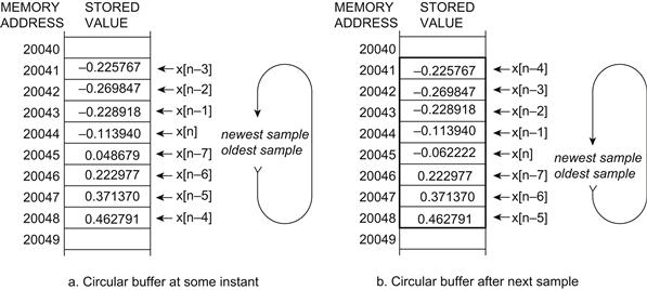
Figure 4-1: Circular buffers are quite often used to store the most recent values of a continuously updated signal.
Since DSPs are commonly used in portable devices that operate on battery power, system resources are often at a premium. Program memory is one such resource that often comes at a premium. In the case of mobile cellular handsets, it is often desirable for the compiler to reduce the size of the program executable as much as possible to fit in the limited program memory resources. At the same time, performance of the DSP kernels is critical and often performance cannot be sacrificed for the sake of program size in memory. Therefore, most DSPs often have multiple encoding schemes. Examples of this include the Arm Thumb2 encoding scheme, as well as the Freescale StarCore SC3850 DSP architecture. In these architectures, instructions are classified into ‘premium’ groupings, whereby powerful instructions that are commonly used within an application are given both a standard 32-bit encoding, as well as a premium 16-bit encoding. When the compiler is compiling for program size optimization, it will attempt to select those instructions that have a premium encoding, requiring fewer bits, in order to conserve program memory requirements of the executable. It should be noted, however, that instructions may be limited in their functionality when they are implemented using premium encoding. Since the instruction is represented with fewer bits in memory, the number of variants that can be encoded in the limited bitset is often reduced. As such, premium encodings of instructions may limit the set of registers that may be used as input and output operands for the instructions. In some cases, there may be implicit couplings between register operands as well; for instance, input registers may be required to be contiguous such as register pairs R0, R1, or R2, R3. Lastly, such premium encodings may reduce the total number of operands and instead overwrite input operands with the output value. Examples of this would be absolute value instructions that are represented as ‘ABS R0, R1’ in a normal encoding, where R0 is the input value, and R1 is the output value. In a premium encoding, the instruction would be represented as ‘ABS R0’, where R0 is the input operand, and the value is destroyed after execution by being overwritten with the output operand. As such, while the encoding may be smaller and reduce program memory requirements, performance of code may deteriorate by some degree due to extra copy operations that may be required to preserve the input value for later use in computation.
Most DSP architectures contain deep processor pipelines requiring multiple clock cycle execution of multiply instructions, and containing rather large branch delay slots on change of flow instructions. For example, the Texas Instruments C6400 series DSPs have a four cycle branch delay slot, which can be costly to program performance if not filled with computation by the compiler, or manually by the assembly programmer. This problem is only exacerbated by the lack of out-of-order execution hardware on most modern DSP architectures as well.
Predicated execution
In order to circumvent costly change of flow instructions required to process control code commonly containing if-then-else statements, many modern DSP architectures contain predicated instructions. Predicated execution is a mechanism whereby the execution of a given instruction is predicated with data values within the processor. In doing this, short branches within the program that may be utilized to implement if-then-else conditions within a C-program, are avoided and bubbles associated with the delay slots of the branch instructions do not deteriorate program performance at runtime. Rather than skip over and branch around the short sections of code in the ‘then’ or ‘else’ conditions, predicated processors simply execute the code contained in all clauses of the if-then-else statement. This effectively permits the processor to execute both branch code paths simultaneously without the performance penalties associated with executing the branch instructions. Control flow in the program is converted into data dependencies within the program via the predication bits associated with each instruction in the various clauses of the control flow statement.
Typically, predicated execution is handled behind the scenes from the application writer by the optimizing compiler. The compiler will often convert control flow dependences within the program to data dependences on predicate registers, or predicate bits within the architecture. As such, costly branching instructions can be avoided at runtime. In predicated DSP architectures, with the appropriate hardware support, the behavior of an operation changes according to the value of the previously computed value or ‘predicate.’ In using predication, multiple regions of the control flow graph are converted into a single region containing predicated code, or instructions. In effect, what were previously control dependences are converted into data dependences. However, given an optimizing compiler, the user does not need to worry about this in their input source code.
In the case of full instruction set predication, instructions take additional operands that determine at runtime whether they should execute or simply be ignored when executed through the DSP’s pipeline. The additional operands are predicate operands, or guards. In the case of partial instruction set predication, special operations, such as conditional move instructions, achieve similar results.
There are a number of compiler techniques available to support predicated execution. They include if-conversion, logical reductions of predicate registers, reverse if-conversion, and hyperblock-based scheduling. Modulo scheduling also falls into this category.
In many embedded systems, predicates are implemented using the general scalar registers of the machines. In other system designs, the predicates are implemented using status bits within control registers. In either case, predicate register real estate is a precious and limited commodity within the system. As such, often the compiler will attempt to reduce the number of predicates needed for a given region of code
An example of a modern predicated architecture used for DSP workloads is the ARM instruction set, which includes a 4-bit set of condition code predicates. The Texas Instruments C6x architecture also supports full predication, with five of the general purpose registers used for predicate values.
Figure 4-2 illustrates a segment of control flow, where the runtime behavior of the program is dependent on whether or not the variable STATUS is set to ACTIVE. If STATUS equals ACTIVE, then the if-statement executes; otherwise the else-statement executes.
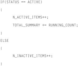
Figure 4-2: Runtime behavior of the program is dependent on whether or not the variable STATUS is set to ACTIVE.
Figure 4-3 shows the pseudo-assembly code generated in the standard case under which predicated execution is not used. As can be seen, the test for equivalence to ACTIVE is performed by the CMP.NEQ instruction, followed by a branch to the relevant control flow destination. The else-statement also contains a branch instruction to the join point labeled ‘JOIN.’
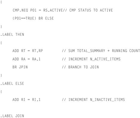
Figure 4-3: Pseudo-assembly code generated in the standard case under which predicated execution is not used.
Figure 4-4 shows the same source code now compiled with support for predicated execution. Notice the use of registers P00 and R01 as predicates. The CMP.EQ instruction is used to set the values of P00 and P01 to true and false, respectively, and these are used as guards on subsequent instructions that were previously part of the if-statements control flow. In this case, both the then-clause and else-clause of the if-statement are executed in parallel since the instructions from each are guarded by P00 and P01, effectively compressing the critical path length of the control-flow statement, and removing all branch instructions and associated delay slots from the control flow statements.
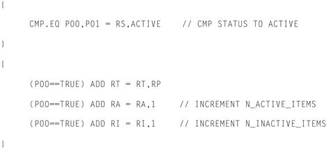
Figure 4-4: Source code compiled with support for predicated execution.
Memory architecture
Most programmable DSP cores today utilize specialized memory architectures that can fetch multiple data and instruction elements per clock cycle. It is often desirable to have architectures for which load and store instructions are the only ones that may access memory. In doing so, it is left up to the compiler to arrange the rest of the work as regards how to use them. If an architecture is allowed memory operands, this will create barriers to instruction level parallelism for the compiler, due to the latency of memory operations and possible data dependences through memory. As such, most DSPs vary in terms of addressing modes, access sizes and alignment restrictions on access to memory.
The addressing modes of the DSP architecture form the basis of the address generation unit. The most common addressing modes for programmable DSP architectures are as follows:
• Register addressing – a register entry within the register file is used as the address pointer.
• Direct or absolute addressing – the address is part of the instruction itself, and the programmer specifies the address within the instruction.
• Register post increment – the address pointer will take a register value and increment this value by a default ‘step’ value.
• Register post decrement – the address pointer will take a register value and decrement this value by a default ‘step’ value.
• Segment plus offset – the address pointer will take a register value added with a defined offset from the instruction.
• Indexed addressing – the address pointer will take a register value and add an indexed register value.
Additionally, there are two other modes of addressing that are common, not only to VLIW architectures, but specifically to DSP architectures. Modulo addressing mode is an addressing mode, mentioned previously, that forces the memory to be used as a FIFO or cyclic ring buffer. Finite Impulse Response filters are typically the most common use of modulo addressing modes, whereby FIFO structures are implemented directly in memory and make use of the modulo addressing capabilities of the DSP core.
Bit reversed addressing mode is another addressing mode that is common to DSP architectures. Fast Fourier Transform is another key kernel that requires high performance in DSPs.
Access sizes
Most modern DSP architectures are capable of accessing memory at varied data widths that are native to the machine’s computation. For example, many DSP architectures can access 8/16/32 bit data operands. In addition, the architectures can also often access 20-bit and 40-bit operands as well, should the architecture provide such data resolution. This is often the case for operations such as multiply accumulate, whereby the bit width resolution of the output operands is higher than that of the input operands. Lastly, due to the VLIW nature of most DSP architectures, they are often capable of accessing packed data elements from memory. For instance, a given DSP architecture that has 128-bit load-store bandwidth, may be able to access 16, 16-bit operands in parallel from memory in one SIMD vector. This is often desirable for computational kernels with high levels of instruction level parallelism, whereby multiple instructions can execute across the multiple VLIW ALUs in parallel.
Alignment issues
As was mentioned above, many VLIW architectures are capable of executing load and store operations of multiple data elements in parallel from memory. This is very useful where there is significant instruction level parallelism. By accessing multiple elements in parallel, and computing across them with SIMD instructions, the ratio of instructions in the program to computation performed is decreased, thereby yielding higher performance.
One challenge in achieving such performance scenarios is the underlying memory system of the DSP architecture. Often, DSP architectures have memory alignment restrictions which ensure that a given memory access exists on certain memory alignment boundaries. Structures may or may not align cleanly to word boundaries. Consider, for example, a structure containing an array of bytes! Additionally, it is common for a program to operate on randomly selected sections within an array, which again causes alignment problems at runtime. A common solution to the alignment restriction of many embedded systems is for the build tools to perform ‘versioning’ at compilation time. In essence, a given loop will have two versions generated in the executable. A switch test is performed at runtime to test whether or not the data is aligned, and if so, the optimized version of the loop is executed. In the event that the switch test determines that data is not aligned at runtime, the non-optimized version of the loop is executed. While this can result in performance improvements at runtime on systems with alignment restrictions that cannot be guaranteed to be met at runtime, there are the obvious trade-offs in executable code size. Another common solution to this is to provide the programmer with ‘pragma’ statements that communicate to the build tools that alignment restrictions are guaranteed to be enforced.
Data operations
Most modern DSP architectures contain a mix of arithmetical operations to meet the varied needs of application developers. It is common for almost all programmable DSP cores to support integer computation. While this portion of the DSP’s instruction set may be used for the signal processing portion of the application being run, it is also used to map the semantics of the C-like programming language onto the DSP cores.
The integer portion of the instruction set is often supplemented with other forms of computation targeted at the DSP portion of the application. Many DSPs include native floating point operations. It should be noted that full IEEE compliance and double precision are rarely characteristic of embedded applications, rather relying on single precision floating point operations. It is often sufficient to omit various IEEE rounding modes and exception handling on floating point operations for the needs of embedded computing. Furthermore, many devices simply opt to emulate floating point computation via software libraries, if native floating point is not a driving requirement. This is only a viable solution when floating performance is not on the critical path of the application, as emulation of floating point instructions in software can often take hundreds of clock cycles on the native VLIW host processor.
It is common for many DSP architectures to support fixed point arithmetic instead of floating point arithmetic. Fixed point data formats are not quite the same as integer data formats. Fixed point format is used to represent numbers that lie between zero and one, with the decimal point assumed to reside after the most significant bit. The most significant bit in this case contains the sign of the number. The size of the fraction represented by the smallest bit is the precision of the fixed point format. The size of the largest number that can be represented by the fixed point format is the dynamic range of the format.
To efficiently use the fixed point format, the programmer must explicitly manage how the data is handled at program runtime. If the fixed point operand becomes too large for the native word size, the programmer will have to scale the number down by shifting to the right. In doing this, lower precision bits may be lost. If the fixed point operand becomes too small, the number of bits actually representing the number is reduced as well. As such, the programmer may decide to scale the number up so as to benefit from an increased number of bits representing the number. In both cases, it is the responsibility of the programmer to manage how many bits are being used to represent the number.
One last data format worth mentioning is the use of saturating arithmetic in DSP architectures. The C programming language semantics imply wraparound behavior for integer data types. However, in many embedded application spaces, such as audio and video processing, it is desirable to have the operands saturate at a maximum or a minimum value. Hardware support for this has both its pros and cons. While an instruction set that has native support for saturating arithmetic can efficiently pipeline such operations, supporting equivalent functionality via min() and max() operations in software can be performed as well. While the compute time is longer to use explicit min() and max() instructions, this may be a sufficient solution for architectures which do not rely on saturating arithmetic for the majority of their computation.
One caveat to supporting saturating arithmetic, without a corresponding non-saturating variant within the instruction set is that, for programmers, the resulting functionality can be confusing and error prone. Consider, for example, computation that is in wraparound mode, and reordered by the build tools at optimization time. Since wraparound mode instructions preserve their arithmetic properties, such as commutativity and associativity at runtime, perceived behavior is not altered when the program is optimized. In the case where the saturating variant of the instructions is used, however, the build tools may either be prohibited from optimizing such computation, or the user may see variance in the output at the bit compatibility level, due to reorderings on the computation performed at optimization time. This can often be difficult to manage for both the end programmer as well as the tools developers.