
Chapter 5
FPGA in Wireless Communications Applications
Chapter Outline
Spatial multiplexing MIMO systems
Tree Traversal for Flex-Sphere detection
Modified real-valued decomposition (M-RVD) ordering
FPGA design of the configurable detector for SDR handsets
Modified real-valued decomposition (M-RVD)
Xilinx FPGA implementation results for MT![]() =
=![]() 3
3
Xilinx FPGA implementation results for MT![]() =
=![]() 4
4
Beamforming in wideband systems
Computational requirements and performance of a beamforming system
Introduction
In the past decade we have witnessed explosive growth in the wireless communications industry with over 4 billion subscribers worldwide. While first and second generation systems focused on voice communications, third generation networks (3GPP and 3GPP2) embraced code division multiple access (CDMA) and had a strong focus on enabling wireless data services. As we reflect on the rollout of 3G services, the reality is that first generation 3G systems did not entirely fulfill the promise of high-speed transmission, and the rates supported in practice were much lower than those claimed in the standards. Enhanced 3G systems were subsequently deployed to address the deficiencies. However, the data rate capabilities and network architecture of these systems were insufficient to address the insatiable consumer and business sector demand for the nomadic delivery of media and data-centric services to an increasingly rich set of mobile platforms.
With these considerations in mind, the move to 4G technologies like 3G LTE (long term evolution) [1] and WiMAX [2] is proceeding at an extremely rapid rate. The goal of next generation systems is to provide high-data rate, low-latency, and high reliability (minimizing outages and connection drops), employing packet-optimized radio access technology, supporting flexible bandwidth allocation. Additional key objectives are to drive down the cost of infrastructure equipment and consumer terminals and to employ a more efficient modulation scheme than the CDMA technology used in 3G systems, in order to make more optimal use of precious communication bandwidth.
To meet all of these requirements a significant re-structuring of both the physical layer (PHY) and network architecture is required. Increased spectral efficiency is delivered in all 4G cellular broadband systems through the use of orthogonal frequency division multiplexing (OFDM) as the preferred modulation scheme. The technology center-piece for delivering improved data rates and communication link robustness lies in more aggressive use of the spatial dimension of communication systems through multiple-input multiple-output (MIMO) techniques [3]. 4G wireless systems will employ MIMO processing to equip next generation systems with spatial multiplexing (improved data rates) and diversity (improved reliability) capabilities. MIMO systems (Figure 5-1) can increase the data rate and provide multiplexing gain by transmitting different data on different antennas [4], also known as spatial multiplexing. MIMO systems can also improve the reliability and error performance in the receiver through diversity gain, i.e., by providing the receiver with multiple copies of the transmitted signal. One practical way to realize such diversity gains is to beamform a message across multiple transmit antennas [5, 6]. The beamforming procedure utilizes limited information about the channel state information; this channel information is usually provided through a limited feedback link from the receiver to the transmitter.
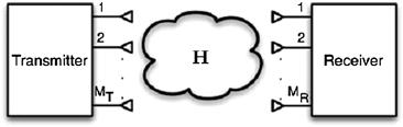
Figure 5-1: Multiple antenna (MIMO) system.
The implementation of 4G infrastructure equipment has several challenges. The first is related to the compute requirements of MIMO-OFDM systems. The more sophisticated MIMO-OFDM advanced receiver architectures have compute requirements that are several orders of magnitude greater than those of 3G CDMA systems. A second requirement is related to bridging the gap between legacy standards (e.g., 3GPP) and next generation 4G protocols and systems. In many cases 4G infrastructure equipment will need to have multi-mode capability and support not only the MIMO-OFDM PHY of WiMAX and 3G LTE systems, but also the W-CDMA (wideband CDMA) PHY of 3GPP-based networks. The silicon technologies deployed in next generation systems will not only need to supply enormous compute capability (many hundreds of giga-operations/second), but they will also require significant flexibility in order to support multi-mode base station infrastructure equipment.
Field programmable gate arrays (FPGAs) with their inherently parallel structure are increasingly the technology of choice for addressing the compute and flexibility requirements of next generation systems. One of the fundamental areas in many academic and industrial research organizations is that of hardware realization of advanced MIMO receivers.
Spatial multiplexing MIMO systems
We assume a MIMO OFDM system with MT transmit antennas and MR ≥ MT receive antennas. We denote the K subcarriers by the subscript k = 1, …, K throughout this chapter. The input-output model is captured by:
![]() (1)
(1)
where ![]() is the complex-valued MR × MT channel matrix,
is the complex-valued MR × MT channel matrix,![]() is the MT -dimensional transmitted vector, where each
is the MT -dimensional transmitted vector, where each ![]() , j = 1, …, MT, is chosen from a complex-valued constellation Ωj of the order wj,k = |Ωj,k|,
, j = 1, …, MT, is chosen from a complex-valued constellation Ωj of the order wj,k = |Ωj,k|, ![]() is the circularly symmetric complex additive white Gaussian noise vector of size MR, and
is the circularly symmetric complex additive white Gaussian noise vector of size MR, and ![]() is the MR-element received vector. Note that we do not restrict all the parallel MT streams to use the same modulation order; rather, each stream, which corresponds to one of the antennas of one of the users, may be using either the 4-, 16-, or 64-QAM modulation. Also, note that even though we focus on one transmitter with multiple antennas, the results in this section can be extended to multiple users such that the sum of the number of antennas of all of them equals MT.
is the MR-element received vector. Note that we do not restrict all the parallel MT streams to use the same modulation order; rather, each stream, which corresponds to one of the antennas of one of the users, may be using either the 4-, 16-, or 64-QAM modulation. Also, note that even though we focus on one transmitter with multiple antennas, the results in this section can be extended to multiple users such that the sum of the number of antennas of all of them equals MT.
We assume that the complete channel information, i.e., the channel matrix coefficients for each subcarrier, are known in the receiver. Moreover, since the detection procedure for each subcarrier is performed independently of other subcarriers, we will drop the k subscript unless it is needed.
Therefore, the original MIMO model can be simplified to ![]() .
.
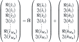
The preceding MIMO equation can be further decomposed into real-valued numbers as follows [7]:
![]() (2)
(2)
corresponding to:
![]() (3)
(3)
with M = 2MT and N = 2MR presenting the dimensions of the new model. We call the ordering in (2) the conventional ordering. Using the conventional ordering, all the computations can be performed in real values, which would simplify the implementation complexity. Note that after real-valued decomposition, each si, i = 1, …, M, in s is chosen from a set of real numbers, Ωi′, with p′i = √pi elements. For instance, for a 64-QAM modulation, each si can take any of the values in the set Ω′ = {±7, ±5, ±3, ±1}. The general optimum detector for such a system is the maximum-likelihood (ML) detector which minimizes ![]() y−Hs
y−Hs ![]() 2 over all the possible combinations of the s vector. Notice that for high order modulations and large number of antennas, this detection scheme incurs an exhaustive exponentially growing search among all the candidates, and is not practically feasible in a MIMO receiver. However, it has been shown that using the QR decomposition of the channel matrix, the distance norm can be simplified [8, 9, 10] as follows:
2 over all the possible combinations of the s vector. Notice that for high order modulations and large number of antennas, this detection scheme incurs an exhaustive exponentially growing search among all the candidates, and is not practically feasible in a MIMO receiver. However, it has been shown that using the QR decomposition of the channel matrix, the distance norm can be simplified [8, 9, 10] as follows:
 (4)
(4)
where H = QR, QQH = I, and y′ = QHy. Note that the transition in (4) is possible through the fact that R is an upper triangular matrix.
The norm in (4) can be computed in M iterations starting with i = M. When i = M, i.e., the first iteration, the initial partial norm is set to zero, TM+1(s(M+1)) = 0. Using the notation of [11], at each iteration the Partial Euclidean Distances (PEDs) at the next levels are given by
![]() (5)
(5)
With s(i) = [si,si+1,…,sM]T, and i = M,M−1,…,1,where
![]() (6)
(6)
![]() (7)
(7)
One can envision this iterative algorithm as a tree traversal with each level of the tree corresponding to one i value, and each node having p′i children.
The tree traversal can be performed in either a breadth-first or a depth-first manner. In the depth-first tree search [12, 11, 13], only one node is expanded at any time and once the end of the tree is reached, the traversal continues by visiting the new nodes in the higher levels of the tree. Therefore, each level can be visited more than one time.
In the breadth-first tree search [14, 15], however, each level is only visited once, and more than one node per level is expanded. Once the end of the tree, or the leaves level, is reached, the minimum candidate is chosen. A typical breadth-first tree search is the K-best detector. In the K-best detector, at each level, only the best K nodes, i.e. the K nodes with the smallest Ti, are chosen for expansion. Note that such a detector requires sorting a list of size K × p′ to find the best K candidates. For instance, for a 16-QAM system with K = 10, this requires sorting a list of size K × p′ = 10 × 4 = 40 at most of the tree levels. This introduces a long delay for the next processing block in the detector unless a highly parallel sorter is used. Highly parallel sorters, on the other hand, consist of a large number of compare-select blocks, and result in dramatic area increase.
Flex-Sphere detector
In order to simplify the sorting step, which significantly reduces the delay of the detector, a sort-free strategy can be utilized. Moreover, we discuss how using a new modified real-valued decomposition ordering (M-RVD) scheme can help in designing a flexible architecture. Finally, we discuss the design and implementation of the flexible sphere detector, Flex-Sphere [16, 17], that can support a range of modulation orders and number of antennas.
Tree Traversal for Flex-Sphere detection
Using the sort-free technique, the long sorting operation is effectively simplified to a minimum-finding operation [16, 18]. The detailed steps of this algorithm are described in the Flex-Sphere Tree Traversal algorithm.
Algorithm 1: Flex-Sphere Tree Traversal

An example of this algorithm is illustrated in Figure 5-2 for a 4 × 4, 64-QAM system. Note that, as described above, the first two levels are fully expanded to guarantee high performance; whereas for the following levels, only the best candidate in the children list of a parent node is expanded. In other words, after passing the first two levels, pMT nodes are expanded, and for each of those pMT nodes, the best child node among its p′M children nodes is selected as the survived node. Therefore, the new node list would contain pMT nodes in the third level. These pMT nodes are expanded in a similar way to the fourth level, and this procedure continues until the very last level, where the minimum-distance node is taken as the detected node.
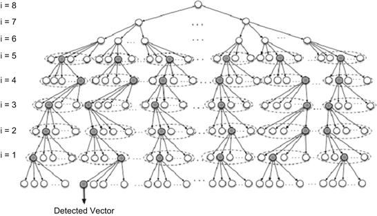
Figure 5-2: Flex-Sphere algorithm for a 64-QAM, 4 × 4 system. The topmost two levels are fully expanded. The nodes marked with black are the minimum in their own set, where each set is denoted by a dashed line. Note that because of the real-valued decomposition, each node has only M=2×MT = 8.
Moreover, from the Schnorr-Euchner (SE) ordering [19], we know that finding
![]()
basically corresponds to finding the real-valued constellation point closest to
![]()
See equation (7). Thus, the long sorting of K-best is avoided.
Modified real-valued decomposition (M-RVD) ordering
For the sort-free detector described in the preceding section, we can use a modified real-valued decomposition (M-RVD) ordering which improves the BER performance compared to the ordering given in equation (2). The new decomposition is summarized as [20]:
![]() (8)
(8)
or,
 (9)
(9)
where ![]() is the permuted channel matrix of equation (3) whose columns are reordered to match the other vectors of the new decomposition ordering in equation (8). It is worth noting that since the difference between RVD and M-RVD is the grouping of the signals, there is no extra computational cost associated with this modified ordering. We will see in the following sections how this ordering could reduce the latency for Flex-Sphere.
is the permuted channel matrix of equation (3) whose columns are reordered to match the other vectors of the new decomposition ordering in equation (8). It is worth noting that since the difference between RVD and M-RVD is the grouping of the signals, there is no extra computational cost associated with this modified ordering. We will see in the following sections how this ordering could reduce the latency for Flex-Sphere.
FPGA design of the configurable detector for SDR handsets
In this section, the main features of the architecture and the FPGA implementation of the SDR handset detector are presented. We use the Xilinx System Generator [21] to implement the proposed architecture. In order to support all the different numbers of antenna/user and modulation orders, the detector is designed for the maximal case, i.e., MT × MR, 64-QAM case, and configurability elements are introduced in the design to support different configurations.
PED computations
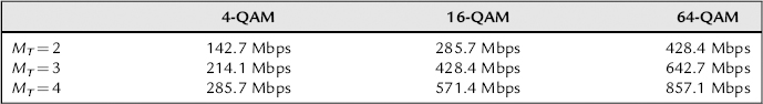
Computing the norms in (7) is performed in the PED blocks. Depending on the level of the tree, three different PED blocks are used: The PED in the first real-valued level, PED, corresponds to the root node in the tree, i = M = 2MT = 8. The second level consists of 64 = 8 parallel PED2 blocks, which compute 8 PEDs for each of the 8 PEDs generated by PED1, thus, generating 64 PEDs for the i = 7 level. Followed by this level, there are 8 parallel general PED computation blocks, PEDg, which compute the closest node PED for all 8 outputs of each of the PED2s. The next levels will also use PEDg. At the end, the Min Finder unit detects the signal by finding the minimum of the 64 distances of the appropriate level. The block diagram of this design is shown in Figure 5-3.
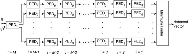
Figure 5-3: The block diagram of the Flex-Sphere. Note that there are M parallel PEDs at each level. The input to the Minimum Finder is fed from the appropriate PED block.
Configurable design
In order to ensure the configurability of the Flex-Sphere, it needs to support different MT as well as different modulation orders for different users. The configurability of the detector is achieved through two input signals, MT and q(i), which control the number of antennas and the modulation order, respectively. These two inputs can change based on the system parameters at any time during the detection procedure. Therefore, this configurability is a real-time operation.
Number of Antennas
The MT determines the number of detection levels, and it is set through MT input to the detector, which in turn, would configure the Min Finder appropriately. Therefore, the minimum finder can operate on the outputs of the corresponding level, and generate the minimum result. In other words, the multiplexers in each input of the Min Finder block choose which one of the four streams of data should be fed into the Min Finder. Therefore, the inputs to the Min Finder would be coming from the i = 5, 3 or 1, if MT is 2, 3, or 4, respectively, (see Figure 5-3).
The MT input can change on-the-fly; thus, the design can shift from one mode to another mode based on the number of streams it is attempting to detect at any time. Moreover, as will be shown later, the configurability of the minimum finder guarantees that less latency is required for detecting a smaller number of streams.
Modulation Order
In order to support different modulation orders per data stream, the Flex-Sphere uses another input control signal q(i) to determine the maximum real value of the modulation order of the i-th level. Thus, q(i) ∈ {1, 3, 7}. Moreover, since the modulation order of each level is changing, a simple comparison-thresholding can not be used to find the closest candidate for Schnorr-Euchner [19] ordering. Therefore, the following conversion is used to find the closest SE candidate:
![]() (10)
(10)
where [.] represents rounding to the nearest integer, J = (1/Rii) · Ji+1 of equation (7), and g(.) is:
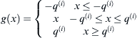 (11)
(11)
All of these functions can be readily implemented using the available building blocks of the Xilinx System Generator (see Figure 5-4). Note that the multiplications/divisions are simple one-bit shifts.
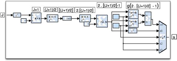
Figure 5-4: The pipelined System Generator block diagram for equation (10) in the PEDg to support different modulation orders.
For the first two levels, which correspond to the in-phase and quadrature components of the last antenna, the PED of the out-of-range candidates are simply overwritten with the maximum value; thus, they will be automatically discarded during the minimum-finding procedure.
Modified real-valued decomposition (M-RVD)
Using the real-valued decomposition, the two extra adders that are required for each complex multiplication can be avoided, thus avoiding the unnecessary FPGA slices on the addition operations. Moreover, while using the complex-valued operations requires the SE ordering of [11], which would be a demanding task given the configurable nature of the detector, with the real-valued decomposition, the SE ordering can be implemented more efficiently and simply for the proposed configurable architecture as described earlier. Also, note that even though some of the multiplications can be replaced with shift-adds in an area-optimized ASIC design, for an FPGA implementation, the appropriate design choice is to use the available embedded multipliers, commonly known as XtremeDSP and DSP48E in Virtex-4 and Virtex-5 devices.
It is noteworthy that if the conventional real-valued decomposition of (3) were employed, then the results for a 2 × 2 system would have been ready only after going through all the in-phase tree levels and the first two quadrature levels. However, with the modified real-valued decomposition (M-RVD), each antenna is isolated from other antennas in two consecutive levels of the tree. Therefore, there is no need to go through the latency of the unnecessary levels. Thus, using the M-RVD technique offers a latency reduction compared to the conventional real-valued decomposition.
Timing analysis
Each of the PEDg blocks are responsible for expanding 8 nodes; thus, the folding factor of the design is F = 8. In order to ensure a high maximum clock frequency, several pipelining levels are introduced inside each of the PED computation blocks. The latency of the PED1, PED2, and PEDg blocks are 7, 17, and 22, respectively. Note that the larger latency of the PEDg blocks is due to more multiplications required to compute the PEDs of the later levels. The Min Finder block has a latency of 8.
As mentioned earlier, different values of MT require different numbers of tree levels, which incurs different latencies. The latencies of the three different configurations of MT are presented in Table 5-1. In computing the latencies, an initial 8 cycles are required to fill up the pipeline path.
Table 5-1: Latency for different values of MT.
| MT | Latency |
| MT = 2 | 8 + PED1 + PED2 + 2 · PEDg + Min_Finder = 84 |
| MT = 3 | 8 + PED1 + PED2 + 4 · PEDg + Min_Finder = 128 |
| MT = 4 | 8 + PED1 + PED2 + 6 · PEDg + Min_Finder = 172 |
Xilinx FPGA implementation results for MT =3
=3
Table 5-2 presents the System Generator implementation results of the Flex-Sphere on a Xilinx Virtex-4 FPGA, xc4vfx100-10ff1517 [21] for 16-bits precision. The maximum number of detectable streams is set to MT = 3. The maximum achievable clock frequency is 250 MHz. Since the design folding factor is set to F = 8, the maximum achievable data rate, i.e., MT = 3 and pi = 64, is:
![]() (12)
(12)
Table 5-2: FPGA resource utilization summary of the proposed Flex-Sphere for the Xilinx Virtex-4, xc4vfx100-10ff1517 device.
| No. of Antennas | 2, 3 |
| Modulation Order | {4, 16, 64}-QAM |
| Max. Data Rate | 562.5 Mbps |
| Number of Slices | 18,825/42,176 (44%) |
| Number of Slice FFs | 23,961/84, 352 (28%) |
| Number of LUTs | 30,297/84, 352 (35%) |
| Number of DSP48E | 129/160 (80%) |
| Max. Freq. | 250 MHz |
Xilinx FPGA implementation results for MT=4
Table 5-3 presents the System Generator implementation results of the Flex-Sphere on a Xilinx Virtex-5 FPGA, xc5vsx95t-3ff1136 [21] for 16-bits precision and MT = 4. The maximum achievable clock frequency is 285.71 MHz. Since the design folding factor is set to F = 8, the maximum achievable data rate, i.e., MT = 4 and pi = 64, is:
![]() (13)
(13)
Table 5-3: FPGA resource utilization of the proposed Flex-Sphere.
| Device | XC5VSX95 |
| No. of Antennas | 2, 3, 4 |
| Modulation Order | {4, 16, 64}-QAM |
| Max.Data Rate | 857.1 Mbps |
| BER = 10-4 @ SNR = | = 25 dB |
| Number of Slices | 11,604/14,720 (78%) |
| Number of Registers/FFs | 27, 115/58,880 (46%) |
| Number of Slice LUTs | 33, 427/58,880 (56%) |
| Number of DSP48E/Multipliers | 321/640 (50%) |
| Number of block RAMs | 0(0%) |
| Max. Freq. | 285.71 MHz |
The Flex-Sphere can support different numbers of antennas and modulation orders, and achieves high data rate requirements of various wireless standards. Table 5-4 summarizes the data rates for all of the different scenarios of the MT = 4, Virtex-5 implementation.
Table 5-4: Data rate for different configurations of the 4 × 4.
Simulation results
In this section, we present the simulation results for the Flex-Sphere, and compare the performance of the FPGA fixed-point implementation with that of the optimum floating-point maximum-likelihood (ML) results. The Xilinx System Generator implementation of the Flex-Sphere detector is shown in Figure 5-5. Prior to the M-RVD, introduced earlier, we employ the channel ordering of [22] to further close the gap to ML. Also, we make the assumption that all the streams are using the same modulation scheme. We assume a Rayleigh fading channel model, i.e., complex-valued channel matrices with the real and imaginary parts of each element drawn from the normal distribution.
Figure 5-5: Xilinx System Generator implementation of the Flex-Sphere detector.
In order to ensure that all the antennas in the receiver have similar average received SNR, and none of the users’ messages are suppressed with other messages, a power control scheme is employed. Figure 5-6 shows the simulation results for the maximal 4 × 4 configuration. As can be seen, the proposed hardware architecture implementation performs within, at most, 1 dB of the optimum maximum-likelihood detection.
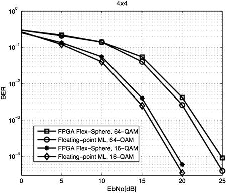
Figure 5-6: BER plots comparing the performance of the floating-point maximum-likelihood (ML) with the FPGA implementation. Note that the channel preprocessing of [22] is employed to improve performance.
Beamforming for WiMAX
Multiple Input Multiple Output (MIMO) antenna systems can be used to increase the data rate (multiplexing gain), improve reliability (diversity gain) or both, in certain combinations [23]. The previous section presented schemes for achieving multiplexing gain. This section explains how full diversity gain is achieved in a WiMAX system via beamforming techniques. Implementation challenges of a beamforming WiMAX system are analyzed and results of experiments performed on an FPGA-based testbed are presented.
MIMO schemes that achieve full diversity gain can be either open loop or closed loop. In a closed loop system, the transmitter has some knowledge of the instantaneous channel realization and if the forward and reverse channels are not reciprocal, the transmitter acquires channel state information from feedback sent by the receiver. Transmit beamforming is an example of a closed loop scheme that achieves full diversity. In an open loop system, the transmitter does not require knowledge of the channel state information; Space Time Codes (STC) are an example of open loop full diversity achieving schemes [24].
The potential for more reliable communication at higher data rates has made closed loop transmit beamforming techniques part of the physical layer of standards for future wireless communications, for example, 802.11n, WiMAX, and 3GPP [25]. Transmit beamforming has been considered in WiMAX Frequency Division Duplexing (FDD) mode, where the forward and feedback channels are not on the same frequency band, hence they are not reciprocal.
Beamforming in wideband systems
The physical layer of the WiMAX standard achieves wideband communication via Orthogonal Frequency Division Multiplexing (OFDM). OFDM is a multicarrier scheme in which subcarriers occupy orthogonal narrowband channels. Beamforming is a narrowband scheme that can be easily extended to wideband OFDM systems by applying beamforming techniques per subcarrier.
Figure 5-7 shows a beamforming OFDM system where channel state information is sent from the receiver to the transmitter via a feedback channel. The system has MT transmitter antennas, MR receiver antennas, and K data subcarriers. ![]() is used to represent the complex symbol transmitted on subcarrier k, 1 ≤ k ≤ K. The time span of the channel impulse response is assumed to be shorter than the time span of the cyclic prefix (this is true for any well designed OFDM system); the baseband relationship between the complex symbol transmitted on subcarrier k and the corresponding received signal yk is given by:
is used to represent the complex symbol transmitted on subcarrier k, 1 ≤ k ≤ K. The time span of the channel impulse response is assumed to be shorter than the time span of the cyclic prefix (this is true for any well designed OFDM system); the baseband relationship between the complex symbol transmitted on subcarrier k and the corresponding received signal yk is given by:
![]() (14)
(14)
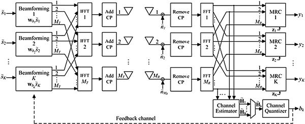
Figure 5-7: Baseband representation of a beamforming MIMO-OFDM system. The FFT and IFFT blocks compute a Fast Fourier Transform and Inverse Fast Fourier Transform respectively. CP is used to denote cyclic prefix.
The MT × 1 vector used for beamforming subcarrier k is represented by wbk. The K beamforming vectors wb1,…, wbK are chosen from a beamforming codebook W of cardinality |W| = 2B, hence, W = {w1,w2,…,w|W|}, and index bk specifies the index of the beamforming vector chosen to beamform subcarrier k, 1 ≤ bk ≤ |W|. The channel matrix corresponding to subcarrier k is represented by the MR × MT matrix ![]() , the entries of
, the entries of ![]() are i.i.d., and each entry is a circularly symmetric complex Gaussian random variable with zero mean and unit variance per complex dimension. To simplify the analysis, it is assumed that the receiver has perfect knowledge of the channel matrix
are i.i.d., and each entry is a circularly symmetric complex Gaussian random variable with zero mean and unit variance per complex dimension. To simplify the analysis, it is assumed that the receiver has perfect knowledge of the channel matrix ![]() . The MR × 1 vector zk is the Maximum Ratio Combining (MRC) vector for subcarrier k. The MR × 1 noise vector
. The MR × 1 vector zk is the Maximum Ratio Combining (MRC) vector for subcarrier k. The MR × 1 noise vector ![]() has i.i.d. entries where each entry is assumed to be circularly symmetric complex Gaussian with zero mean and variance N0 per complex dimension. Each subcarrier is transmitted with the same average power Es; this constraint is met by setting E[
has i.i.d. entries where each entry is assumed to be circularly symmetric complex Gaussian with zero mean and variance N0 per complex dimension. Each subcarrier is transmitted with the same average power Es; this constraint is met by setting E[![]() ] = Es and
] = Es and ![]() wbk
wbk ![]() = 1. The WiMAX standard specifies beamforming codebooks for different numbers of transmitter antennas and codebook cardinalities; all the beamforming vectors in the WiMAX codebooks satisfy
= 1. The WiMAX standard specifies beamforming codebooks for different numbers of transmitter antennas and codebook cardinalities; all the beamforming vectors in the WiMAX codebooks satisfy ![]() wbk
wbk ![]() = 1. (Note that
= 1. (Note that ![]() ·
·![]() is used to denote the vector two-norm and (·)H denotes the conjugate transposition of a matrix.)
is used to denote the vector two-norm and (·)H denotes the conjugate transposition of a matrix.)
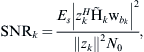
The SNR for subcarrier k is given by:
 (15)
(15)
the MRC vector and the index of the beamforming vector that maximize SNRk are [5]
 (16)
(16)
![]() (17)
(17)
respectively.
In a beamforming FDD system like the one considered in the WiMAX standard, the beamforming codebook W is known to both the transmitter and the receiver. The K indices b1, b2,…,bK computed by the channel quantizer at the receiver are fedback to the transmitter. Based on these indices, the transmitter beamforms subcarriers 1, 2,…, K using vectors wb1, wb2,…,wbK respectively. The K indices b1, b2,…,bK computed by the channel quantizer are also used to compute the MRC vectors as shown in (16). Since the codebook has cardinality |W| = 2B, each index bk is represented using B bits. The total amount of feedback bits is equal to KB, which corresponds to B bits of feedback information per subcarrier. The WiMAX standard specifies different possible mechanisms to send the KB bits of feedback information from the receiver to the transmitter; in some configurations (e.g. adjacent subcarrier permutations [26]) the amount of feedback bits can be reduced by clustering subcarriers.
The process of quantizing each subcarrier channel ![]() into B bits takes place at the channel quantizer. Since each subcarrier goes through an independent channel, each subcarrier channel must be quantized independently. In order to reutilize hardware resources the quantizer processes one subcarrier at a time, as shown in Figure 5-7. The input-output relationship of the channel quantizer is given by equation (17) which is computed by exhaustive searching over the elements in the codebook W.
into B bits takes place at the channel quantizer. Since each subcarrier goes through an independent channel, each subcarrier channel must be quantized independently. In order to reutilize hardware resources the quantizer processes one subcarrier at a time, as shown in Figure 5-7. The input-output relationship of the channel quantizer is given by equation (17) which is computed by exhaustive searching over the elements in the codebook W.
The system depicted in Figure 5-7 achieves full diversity if |W| ≥ MT and the beamforming codebook is designed based on the Grassmannian beamforming criterion [5]. The WiMAX standard specifies codebooks for 2, 3, and 4 transmit antennas. For 2 transmit antennas the WiMAX standard specifies a codebook of size |W| = 8; for 3 and 4 transmitter antennas the standard specifies one codebook of size |W| = 8 and one codebook of size |W| = 64. The WiMAX codebooks seem to be designed based on the Grassmannian criterion [27] and it can be verified via Monte Carlo simulation that WiMAX codebooks achieve full diversity.
Computational requirements and performance of a beamforming system
Implementation of the beamforming and MRC blocks in Figure 5-7 is straightforward; the most intensive computation in each of the blocks is a vector multiplication. Also, the K beamforming and K MRC blocks can be reduced to one beamforming block and one MRC block by processing one subcarrier at a time.
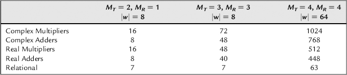
Implementation of the channel quantizer in Figure 5-7 can require a large amount of resources depending on the number of transmitter antennas and codebook size. The entries of ![]() are complex numbers and the WiMAX standard specifies that the entries of wi are complex numbers rounded to four decimal places. Hence, computing
are complex numbers and the WiMAX standard specifies that the entries of wi are complex numbers rounded to four decimal places. Hence, computing ![]() for all the |W| codewords requires |W|MT MR complex multiplications, |W|MT MR −|W|MR complex additions, 2|W|MR real multiplications, and 2|W|MR − |W| real additions. After computing
for all the |W| codewords requires |W|MT MR complex multiplications, |W|MT MR −|W|MR complex additions, 2|W|MR real multiplications, and 2|W|MR − |W| real additions. After computing ![]() for all |W| codewords the channel quantizer searches for the codeword with the largest
for all |W| codewords the channel quantizer searches for the codeword with the largest ![]() . Implementing a tree search requires |W|−1 relational blocks that compare two inputs and then output the greater of the two.
. Implementing a tree search requires |W|−1 relational blocks that compare two inputs and then output the greater of the two.
The total amount of resources required for channel quantization for one subcarrier in different WiMAX configurations is shown in Table 5-5. Notice that as the number of antennas and codebook cardinality increases, the number of resources required increases dramatically. The maximum number of embedded multipliers in an FPGA is 512 for the Xilinx Virtex-4 family [28] and 1056 for the Xilinx Virtex-5 family [29]. Hence, implementing the channel quantizer can become a bottleneck for the implementation of WiMAX systems.
Table 5-5: Resources required for channel quantization.
The amount of resources required for channel quantization can be reduced by reutilizing resources, but resource reutilization would increase the latency of the channel quantizer. Reutilization is possible as long as the timing constraints are met. In a WiMAX system the timing constraints can be quite tight, specially in high mobility scenarios and in frequency division duplexing (FDD) mode. In a high mobility scenario the channel coherence interval decreases and feedback information must be sent before it becomes stale and in FDD mode feedback information can potentially be sent as soon as it is available. In both FDD mode and high mobility the faster the feedback information is sent the more throughput the system will have, since more payload data will be sent during a coherence interval.
Another alternative to reduce the amount of resources required for channel quantization is to use a mixed codebook scheme as proposed in [30]. In a mixed codebook scheme, the WiMAX codebook is used at the transmitter for beamforming and at the receiver for MRC, and a mapped version of the WiMAX codebook is used at the receiver’s channel quantizer. The entries in the mapped version of the WiMAX codebook belong to {0,+1,−1,+j,−j}; hence, all the complex multiplications required for channel quantization can be implemented via simple changes and swapping of the real and imaginary parts of the channel matrix entries. Table 5-6 compares the amount of resources required for channel quantization when using a mapped WiMAX codebook with the amount of resources required when using a WiMAX codebook. The mapped version of the WiMAX codebook can be obtained via the vector mapping proposed in [30]. Using a mixed codebook scheme will affect performance because the codebook used for beamforming at the transmitter and MRC at the receiver is different from the codebook used for channel quantization at the receiver. However, the performance loss is very small, since by construction, the mapped WiMAX codebook has quantization regions similar to the quantization regions of the WiMAX codebook from which it is obtained [30]. Notice that the mixed codebook scheme remains WiMAX compliant because the mapped WiMAX codebook is only used for channel quantization.
Table 5-6: Resources required for channel quantization using a WiMAX codebook and a mapped WiMAX codebook. Results correspond to a system with 4 transmitter and 4 receiver antennas and a codebook of 64 codewords.
| WiMAX Codebook | Mapped WiMAX Codebook | |
| Complex Multipliers | 1024 | 0 |
| Complex Adders | 768 | 768 |
| Real Multipliers | 512 | 576 |
| Real Adders | 8 | 448 |
| Negators | 0 | 2048 |
| 5-input Multiplexer | 0 | 2048 |
| Relational | 63 | 63 |
Observe from Table 5-6 that when using a mapped WiMAX codebook for channel quantization, the number of multiplications required reduces to zero. This reduction is obtained by increasing the number of five input multiplexers and negators (a negator block is a very simple block that computes the arithmetic negation or two’s complement of its input). For both ASIC and FPGA implementations, 2048 five input multiplexers, 2048 negators, and 64 real multipliers require fewer resources than implementing 1024 complex multipliers.
Figure 5-8 shows the performance of different beamforming WiMAX configurations. All simulations were run for a one subcarrier model, and the results obtained represent the per subcarrier behavior in an OFDM system. The results in Figure 5-8 correspond to the best case scenario of perfect channel estimate at the receiver, noiseless and zero delay feedback, and floating-point processing. The results in Figure 5-8 show that in a feedback-based beamforming system, such as FDD WiMAX, few bits of feedback can achieve performance close to the ideal case of infinite feedback. Also, observe that using a mixed codebook scheme (labeled MC in the figure) results in small performance degradation, and as shown in Table 5-6, the amount of resources can be significantly reduced by using a mixed codebook scheme. Figure 5-8 also shows the performance of the Alamouti STC [31], which is an open loop scheme. Observe that the closed loop beamforming scheme outperforms the open loop scheme.
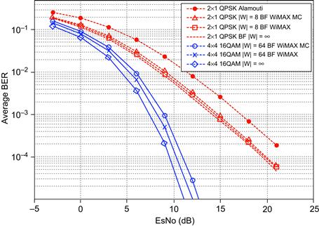
Figure 5-8: Performance of a MT × MR beamforming WiMAX system for different values of MT, MR, and |W|. BF is used to denote beamforming, MC is used to denote mixed codebook scheme, and |W| = ∞ is used to denote an infinite feedback scenario.
Beamforming experiments using WARPLab
WARPLab is a framework for rapid prototyping of physical layer algorithms. The WARPLab framework combines the ease of MATLAB with the capabilities of the Wireless Open Access Research Platform (WARP) developed at Rice University [32]. This section describes in detail the WARPLab framework and presents experiment results that show the performance gains that can be obtained with beamforming in a WiMAX system.
WARPLab framework
WARP provides a unique platform to develop, implement, and test advanced wireless communication algorithms. The platform architecture consists of four main components: custom hardware, platform support packages, open-access repository, and research applications.
The custom hardware allows implementation and scalability of sophisticated signal processing algorithms and provides extensible peripheral options for radios and user interface. The main component of the WARP hardware is a Xilinx Virtex II-Pro FPGA, a new version of the WARP hardware will soon be released, and in this new version, the Xilinx Virtex II Pro FPGA has been replaced by a more powerful Xilinx V-4 FPGA. The WARP board, shown in Figure 5-9, has four daughter card slots and each slot is connected to a dedicated bank of I/O pins on the FPGA, providing a flexible, high-throughput interface. As shown in Figure 5-9, the four daughter card slots can be used to connect the FPGA to four different radio boards so that up to a 4 × 4 MIMO system can be built. The radio boards have been designed by Rice University students and these boards are capable of targeting both the 2.4 GHz and 5 GHz ISM bands. They are intended for wide band applications, such as OFDM, with a bandwidth up to 40 MHz.
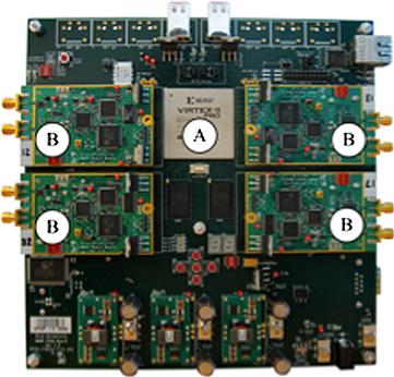
Figure 5-9: WARP board with a radio board in each of the four daughtercard slots. A: Xilinx Virtex-II Pro FPGA. B: Radio board.
The platform support packages facilitate seamless use of the WARP hardware by researchers working at all layers of wireless network design. The open-access repository [33], accessible from the Internet, is the central archive for all source codes, models, platform support packages, application building blocks, research applications, design documents, and hardware design files associated with WARP. The contents of the repository are verified by the project administrator at Rice University.
WARP allows clean-slate design and prototyping of physical layer algorithms for wireless communications via two possible design flows: 1) real time implementation and 2) WARPLab framework that allows real-time RF transmission and offline processing on a host PC. In real-time implementation, all the signal processing is implemented in the FPGA, allowing implementation of a complete end-to-end real-time system. However, many physical layer researchers are interested in rapid prototyping and over-the-air testing of new algorithms without having to deal with the details of FPGA implementation, and without having to implement mechanisms that belong to higher layers, like carrier sensing, contention resolution protocols, and packet detection. To meet these requirements, Rice University has developed the WARPLab framework, which allows generation of waveforms in MATLAB and provides simple m-code functions that allow over-the-air transmission of these waveforms using the WARP hardware.
The basic WARPLab setup is shown in Figure 5-10. Two WARP nodes are connected to a host PC via an Ethernet switch. Up to 16 WARP nodes can be connected to the switch and controlled from the host PC. A user first uses MATLAB to construct waveforms that their algorithm would transmit. These waveforms are loaded into the assigned WARP transmit nodes via Ethernet links that are controlled by custom code on both the PC and WARP nodes. The host PC then triggers the beginning of the experiment by telling the transmit nodes to begin their transmissions and the receive nodes to begin capturing data from the radio. Once transmission and capture are completed, the captured waveforms are passed to the host PC via the Ethernet links. The user can then use MATLAB to process the received waveforms and determine the effects of real radios and wireless channels on their novel algorithm.
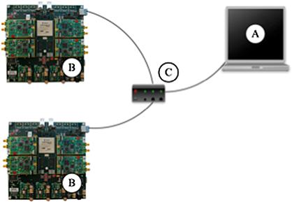
Figure 5-10: Basic WARPLab setup. A: Host PC, B: WARP node, C: Switch. The switch is connected to the WARP nodes and the host PC via Ethernet links.
The WARPLab framework provides the software necessary for easy interaction with the WARP nodes directly from the MATLAB workspace. The software consists of FPGA code and m-code functions which are all available in the WARP repository [34].
Experiment setup and results
This section shows experiment results for a beamforming system with two transmitter antennas and one receiver antenna. The system was designed and tested using the WARPLab framework. Experiments were performed over a wireless channel emulated using Spirent’s SR-5500 wireless channel emulator. The experiment setup is shown in Figure 5-11. Two radios at the transmitter node are connected to the two RF inputs of the channel emulator which emulates two independent RF wireless channels. The two RF outputs of the channel emulator are added to emulate a 2 × 1 system; the output of the RF adder is connected to one radio at the receiver node. The channel emulator is connected to the host computer via Ethernet; the host computer controls the two WARP nodes and the channel emulator via the Ethernet links.
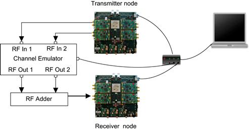
Figure 5-11: Experiment setup. The basic WARPLab setup was connected to a channel emulator and an RF adder to emulate a system with two transmitter antennas and one receive antenna.
The system implemented is a single subcarrier system, the results representing the per subcarrier behavior in an OFDM system. Table 5-7 summarizes the experiment conditions; the two emulated RF channels were both set using exactly the same parameters. Since the delay spread is much smaller than the symbol period, the transmitted signal goes through a flat fading channel.
Table 5-7: Experimental conditions.
| Parameter | Value |
| Number of transmitter antennas | 2 |
| Number of receiver antennas | 1 |
| Carrier frequency | 2.4 GHz |
| Number of subcarriers | 1 |
| Bandwidth | 625 kHz |
| Sampling frequency | 40 MHz |
| Pulse shaping filter | Squared Root Raised Cosine (SRRC) |
| SRRC roll-off factor | 1 |
| Symbol time | 3.2 μs |
| Modulation | 16 QAM |
| Coding Rate | 1 (No error correction code) |
| Energy per symbol | -20 dBm at input of channel emulator |
| Paths per emulated RF channel | 3 |
| Envelope per path | Rayleigh flat fading all 3 paths |
| Fading Doppler per path | 0.1 Hz (0.04 km/h) in all 3 paths emulates block fading channel |
| Delay per path | Path 1=0 μs, Path 2=0.05 μs, Path 3=0.1 μs |
| Relative path loss | Path 1=0 dB, Path 2=3.6 dB, Path 3=7.2 dB |
Transmission of the payload data was done in packets of 110 symbols. The number of symbols per packet was limited to 110 due to the characteristics of the transmitted signal (symbol time of 3.2 μs and sampling frequency of 40 MHz) and the maximum number of samples that can be stored per receiver radio in a node, which is limited to 214 samples [34]. As shown in Figure 5-12, two pilot sequences were sent before transmission of payload. The first pilot sequence was used for computation of the channel estimate used for channel quantization, and the total pilot energy was set equal to twice the energy per symbol. The second pilot sequence was a beamformed pilot sequence, which was used to obtain an estimate of the channel, times the beamforming vector. This estimate was used for MRC at the receiver and the total pilot energy was equal to the total energy per symbol. The error-free feedback channel was implemented in the host PC (the host PC is connected to both transmitter and receiver). The feedback delay was approximately 60 ms, which is the time it took to send training, estimate the channel, quantize the channel estimate, and start transmitting the beamformed signal.
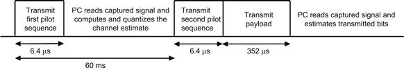
Figure 5-12: Time diagram of transmitted signal and PC processing for beamforming experiment.
In order to compare the performance of a closed loop scheme like beamforming and an open loop scheme like Alamouti, a 2 × 1 Alamouti scheme was also implemented and tested using the WARPLab framework. In the Alamouti scheme, transmission of the payload data was also done in packets of 110 symbols. For the Alamouti implementation, only one pilot sequence was sent and payload was sent immediately after the pilot sequence. The total pilot energy was equal to the total energy per symbol.
Simulation results in Figure 5-8 showed that the beamforming scheme has better performance than the Alamouti scheme and that the mixed codebook scheme for efficient implementation results in small performance degradation. These two observations are verified by the experiment results shown in Figure 5-13. The results also show that, as expected, few feedback bits have performance close to the performance of infinite feedback. Observe that the plots of the experiment results are not as smooth as the plots of the simulation results. This is very likely due to hardware non-linearities and the fact that simulations were run more for total number of bits than were experiments because simulations ran faster.
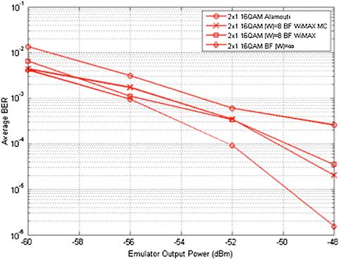
Figure 5-13: Experiment results for a 2 × 1 beamforming system and a 2 × 1 Alamouti system. BF is used to denote beamforming, MC is used to denote mixed codebook scheme, and |W| = ∞ is used to denote an infinite feedback scenario.
Conclusion
In this chapter, we discussed the architectural challenges of spatial multiplexing and diversity gain schemes, and further, introduced FPGA-centric architectures and experiments for these systems. We introduced a flexible architecture and implementation of a spatial multiplexing MIMO detector, Flex-sphere, and its FPGA implementation. We also presented a hardware architecture for beamforming for WiMAX, as a way to enhance the diversity and performance in the next-generation wireless systems. Finally, we showed how we utilized the WARP platform for studying the effects of MIMO systems in real-world scenarios.
REFERENCES
1. [Online]. Available: http://www.3gpp.org/.
2. [Online]. Available: http://wirelessman.org/.
3. Foschini G. Layered space-time architecture for wireless communication in a fading environment when using multiple antennas. Bell Labs Tech Journal. 1996;2.
4. Golden GD, Foschini GJ, Valenzuela RA, Wolniansky PW. Detection algorithms and initial laboratory results using V-BLAST space-time communication architecture. Electronics Letters. 1999;35:14–15.
5. Love DJ, Heath RW, Strohmer T. Grassmannian beamforming for multiple-input multiple-output wireless systems. IEEE Trans Inform Theory. Oct 2003;49:2735–2747.
6. Mukkavilli KK, Sabharwal A, Erkip E, Aazhang B. On beamforming with finite rate feedback in multiple-antenna systems. IEEE Trans Inform Theory. Oct 2003;49:2562–2579.
7. Guo Z, Nilsson P. A 53.3 Mb/s 4 × 4 16-QAM MIMO decoder in 0.35μm CMOS. IEEE Int Symp Circuits Syst. May 2005;5:4947–4950.
8. Damen MO, Gamal HE, Caire G. On maximum likelihood detection and the search for the closest lattice point. IEEE Trans on Inf Theory. Oct 2003;49(no 10):2389–2402.
9. Fincke U, Pohst M. Improved methods for calculating vectors of short length in a lattice, including a complexity analysis. Math Computat. Apr 1985;44(no 170):463–471.
10. Hochwald B, ten Brink S. Achieving near-capacity on a multiple-antenna channel. IEEE Trans on Comm. Mar 2003;51:389–399.
11. Burg A, Borgmann M, Wenk M, Zellweger M, Fichtner W, Bolcskei H. VLSI implementation of MIMO detection using the sphere decoding algorithm. IEEE Journal of Solid-State Circuits. July 2005;40(no 7):1566–1577.
12. Amiri K, Cavallaro JR. FPGA implementation of dynamic threshold sphere detection for MIMO systems. 40th Asilomar Conf on Signals, Systems and Computers Nov 2006.
13. Garrett D, Davis L, ten Brink S, Hochwald B, Knagge G. Silicon complexity for maximum likelihood MIMO detection using spherical decoding. IEEE JSSC. Sep 2004;39(no 9):1544–1552.
14. Guo Z, Nilsson P. Algorithm and implementation of the K-Best sphere decoding for MIMO detection. IEEE JSAC. Mar 2006;24(no 3):491–503.
15. Wong K, Tsui C, Cheng RS, Mow W. A VLSI architecture of a K- best lattice decoding algorithm for MIMO channels. IEEE Int Symp Circuits Syst. May 2002;3:273–276.
16. Amiri K, Cavallaro JR, Dick C, Rao R. A high throughput configurable SDR detector for multi-user MIMO wireless systems. Springer Journal of Signal Processing 2009.
17. Amiri K, Dick C, Rao R, Cavallaro JR. Flex-Sphere: An FPGA Configurable Sort-Free Sphere Detector for Multi-user MIMO Wireless Systems. Proc of SDR Forum Oct 2008.
18. L. G. Barbero and J. S. Thompson, ‘FPGA design considerations in the implementation of a fixed-throughput sphere decoder for MIMO systems,’ Field Programmable Logic and Applications, 2006. FPL ’06. International Conference on, Aug. 2006.
19. Schnorr CP, Euchner M. Lattice basis reduction: improved practical algorithms and solving subset sum problems. Math Programming. Sep 1994;66(no 2):181–191.
20. Amiri K, Dick C, Rao R, Cavallaro JR. Novel sort-free detector with modified real-valued decomposition (M-RVD) ordering in MIMO systems. Proc of IEEE Globecom Dec 2008.
21. [Online]. Xilinx: http://www.xilinx.com/.
22. Barbero LG, Thompson JS. A fixed-complexity MIMO detector based on the complex sphere decoder. IEEE 7th Workshop on Signal Processing Advances in Wireless Communications, 2006 SPAWC ’06 Jul 2006.
23. Zheng L, Tse D. Diversity and multiplexing: A fundamental tradeoff in multiple-antenna channels. IEEE Trans Inform Theory. Oct 2003;49:1073–1096.
24. Tarokh V, Seshadri N, Calderbank AR. Space-time codes for high data rate wireless communication: Performance criterion and code construction. IEEE Trans Inform Theory. 1998;44:44–765.
25. Hottinen A, Kuusela M, Hugl K, Zhang J, Raghothaman B. Industrial embrace of smart antennas and MIMO. IEEE Wireless Communications. Aug 2006;13:8–16.
26. ‘IEEE standard for local and metropolitan area networks part 16: Air interface for fixed and mobile broadband wireless access systems,’ IEEE Std 802.16e–2005 and IEEE Std 802.16-2004/Cor 1-2005, 2006.
27. Love D, Heath R, Lau VKN, Gesbert D, Rao BD, Andrews M. An overview of limited feedback in wireless communication systems. IEEE JSAC. Oct 2008;46:1341–1365.
28. [Online]. Available: http://www.xilinx.com/products/virtex4.
29. [Online]. Available: http://www.xilinx.com/products/virtex5.
30. Duarte M, Sabharwal A, Dick C, Rao R. A vector mapping scheme for efficient implementation of beamforming MIMO systems. MILCOM 2008.
31. Alamouti SM. A simple transmit diversity technique for wireless communications. IEEE JSAC. 1998;16:1451–1458.
32. [Online]. Available: http://warp.rice.edu.
33. [Online]. Available: http://warp.rice.edu/trac.
34. [Online]. Available: http://warp.rice.edu/trac/wiki/WARPLab.