Chapter 17
Developing and Debugging a DSP Application
Chapter Outline
Integrated Development Environment
Build and link the application for a multi-core DSP environment
Compiler configuration for application
Linker configuration for application
Execute and debug the application on multi-core DSP
Set up the launch configuration
Trace and Profile the multicourse application using hardware and software dedicated resources
Integrated Development Environment overview
The CodeWarrior IDE is a complete integrated development environment based on the latest Eclipse platform, designed to accelerate the development of embedded applications.
On top of the Eclipse platform, the specific CodeWarrior plug-ins such as compiler, linker, debugger, and software analysis engine, were implemented in order to provide access to the specific DSP features.
Even more, being an Eclipse based development environment the user is encouraged to use any third party software that can be integrated as a plug-in into the IDE to maximize the user experience in such way that other tools cannot offer. For example, the user might choose to use his own plug-in for source versioning system or his own editor if this makes him more comfortable in using the tool.
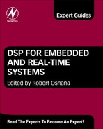
The modular philosophy is depicted in Figure 17-1. Any other 3rd party service which is Eclipse platform compatible can also plug-in into the IDE and the user will reap the benefits of this.
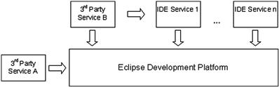
Figure 17-1: CodeWarrior modular architecture overview.
In order to reuse parts of software created for other platforms the IDE specific tools are also created as plug-ins (e.g., the flash programmer is the same plug-in between Power Architecture and StarCore families).
In order to maintain a relative high performance and a good out-of-the-box user experience, some of the critical software components that are part of IDE are built-into Eclipse rather than delivered as standalone plug-ins.
Creating a new project
First time users, who are not familiar with the Eclipse terminology, will find themselves confronted with a new way of doing things compared with other classic development tools. The first thing that the IDE asks when it is opened is the path towards the workspace as depicted in Figure 17-2.
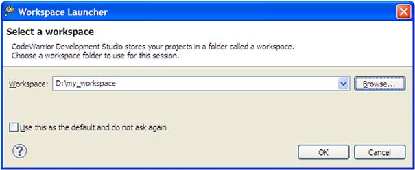
Figure 17-2: Workspace dialogue
The workspace is a container that maintains all the ‘things’ the embedded software engineers need for editing, building, and debugging a project. For each user, the workspace takes the form of locally physical location where the IDE will place the .metadata structure that will hold the project history and configuration tools settings.
The usage of local workspace allows a better and more efficient collaboration between team members and easy exchange of code source through network shared repositories. Each team member can customize his own local workspace in order to accommodate his preferences related with the plug-ins used or the way in which the IDE displays the windows, widgets, text editors, and so forth. After the workspace is created the workbench opens and the user can perform the following actions from a rich set of predefined options.
Enhancements can be made to the default Eclipse stock menus with intuitive actions such as:
• Create a new project with default initializations, DSP start-up code, and JTAG connection
• Import an existent project into workspace
• Migrate an older project type to newest IDE
• Create a new project based on a collection of source files
• Create and characterize a new target connection for debugging purposes
• Create new configurations files for peripherals configuration
Figure 17-3 shows all the options available in the New menu. To create a new project in a couple of simple steps the StarCore Project needs to be used. This menu will guide the user throughout the new project wizard which contains simple actions like:
Figure 17-3: New project menu.
The main steps for a new project wizard are shown in Figure 17-4.
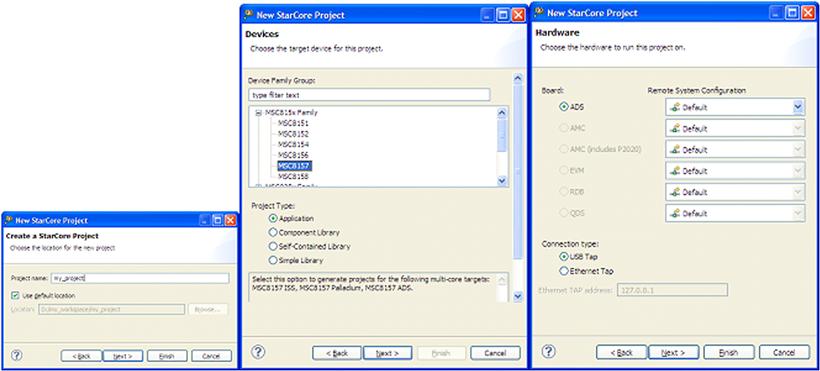
Figure 17-4: New project wizard main steps.
Apart of rich menus and options for supporting different features, the IDE provides a rich set of demos that covers the main hardware capacities. These demos are designed for shortening the development cycle by providing ready-to-run applications, drivers, and APIs.
For demonstration of the software development features in the following sections an application based on SmartDSP OS (SDOS) will be used.
The asymmetric_demo is based on a standard SDOS demo (that can be created via New menu), that has been modified to demonstrate the use of asymmetric memory model for each of the DSP cores and thus enabling each core to run different code and data. The demo also illustrate how to link a multi-core system so that each of the cores have different implementations of the same methods. Additionaly, the usage of software interrupts, times, and specific SDOS functionalities are implemented. Figure 17-5 shows the steps for importing an existing project into the workspace.
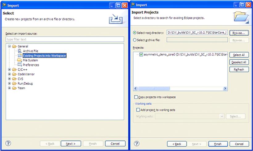
Figure 17-5: Importing existing projects.
The IDE asks the user to specify the path where the projects are located. Then, it automatically updates the list of available projects within the user specified folder. Within a folder, only one single project can reside. For each project there is a pair of two XML files called .project and .cproject. These two files record the project settings like file organization, tools settings, and project properties.
The Import dialogue also requires the user to specify if the IDE should copy the projects from the current location into the active workspace. This is useful when the original project version needs to be preserved.
After the project is imported successfully, the IDE automatically opens the default C/C++ perspective and offers complete overviews of the project resources as in Figure 17-6.
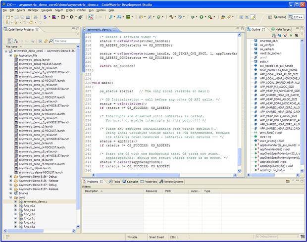
Figure 17-6: Default C/C++ editor perspective.
The term of perspective is borrowed by the IDE from the Eclipse platform and refers to a ‘visual container’ that determines user interactions with the IDE and in the same time offering a task oriented user experience.
The IDE is delivered with two default perspectives:
• C/C++ perspective is designed to offers all the tools needed for software development such as: text editor, project explorer, outline, build console and problem viewer, etc.
• Debug perspective is designed for debugging DSP targets by displaying the main features like stack frames, editors for source and disassembly, variable and register views, output console
Any of the perspectives can be customized by adding or removing the any of the views based on user requirements. The entire list of tools and features supported by the IDE can be accessed via menu Window/Show view/Other, as is shown in Figure 17-7.
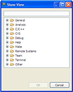
Figure 17-7: List of all available tools.
On the left hand side, the Project panel displays all the files that belong to the asymmetric demo project. Within this panel, the user can control all the project settings and can easily navigate throughout the project files and folders. The user can choose between different modes of file organization within the project since the IDE offers a wide range of features like grouping files in virtual folders or groups (these folders do not exist on the physical drive) or adding links to real files. The IDE offers full control of project files and directories organization.
The overall project or individual file or folder properties can be easily accessible via a simple right click on each the items. The list of actions is displayed in Figure 17-8.
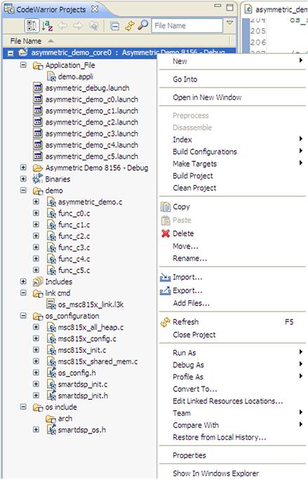
Figure 17-8: List of project editing options.
Build and link the application for a multi-core DSP environment
Before starting to describe the building and linking process for the application considered in the previous chapter, a few details about the SDOS and the application memory map must be presented.
DSP (SDOS) Operating system
SDOS is a real-time operating system designed for DSP build on StarCore technology. It includes: royalty free source code, real-time responsiveness, C/C++/asm support, small memory footprint, support for SDPS family products, and full integration with the IDE.
The main features of the DSP OS include:
• Priority based event-driven scheduling triggered by SW of HW
• Dual-stack pointer for exception and task handling
• Inter-task communication using queues, semaphores, and event
• Designed as a asymmetric multi-processing system where each core runs its own OS instance
• Manages shared resources and supports inter-core communication
The DSP OS architecture is depicted in Figure 17-9. The operating system includes: kernel, peripherals drivers, the Ethernet stack (UDP/TCP/IP) and runtime enablement tools (Kernel awareness, HEAT, eCLI).
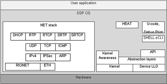
Figure 17-9: DSP operating system architecture.
The SDOS, is integrated into the asymmetric demo project as a component library that needs to be linked with the user application. Apart of the library, SDOS configuration files and headers must be included into the project in order to initialize and configure the OS based on user requirements.
These configurations files are accessible from the IDE Project panel within the os_configuration and os_include virtual folders. The user is free to change any settings starting with the stack and heap sizes up to the settings assocated with OS functionalities like number of running cores, cores synchronizations, cache policies, barriers.
Application memory map
The application, considerer in this analysis, covers the complex topic of the Multi Instruction and Multi Data model. In this case, each core is going to execute private code and handle private data.
This concept permits a complex software design to be broken down into smaller and simpler tasks. Therefore the MIMD design can divide the application processing requirements by distributing a portion of it across all the cores so that the DSP resources are used more efficiently.
The most critical aspect of the application is to divide the DSP resources properly among the tasks. Each memory type available on DSP has specific characteristics and purposes:
• System shared memory – shared among all the processor cores
• Symmetric memory – private to each core but the objects within this memory reside on the same virtual address for all the cores in the system
Beside virtual memory, the user must also choose the physical memory within the system to be used for application purposes. For example, on the Freescale MSC815x the available choices are: M2, M3, DDR0, and DDR1 (see Figure 17-10).
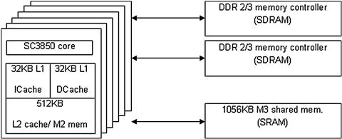
Figure 17-10: Physical memory on MSC815x DSP.
The system engineer needs to consider where each module of the application will be placed into the memory. Each physical resource (see Figure 17-10) must be partitioned by identifying which application modules need to be shared within the system and which modules are private to the cores. The steps required for code and data sections partitioning will be discussed in the next two sub-section that address the compiler and linker options. Specific examples with compiler and linker commands are provided for a better understanding.
In this case the modules that must be shared across all the cores are:
The modules that must be private to each core are:
Figure 17-11 shows the physical memory map of the asymmetric demo project. The user application layer is simulated via func_c(0-5).c modules. Inside these modules the user can insert the custom code that will be run indecently for each of the cores.
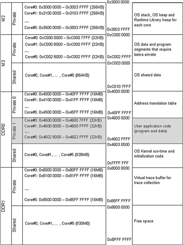
Figure 17-11: Application memory map.
After the DSP platform is started-up, the initializations of SDOS and user application are performed. After all initializations are done, the operation system will start the default background job.
The user function is then called via a software timer created during the application initializations.
Compiler configuration for application
The IDE provides easy and straightforward methods to allocate the code and data so that the application requirements shown in Figure 17-11 are met. The application functions and variables are placed by the compiler in the appropriate sections via the application configuration file (∗.appli).
Alternatively the placement can be done via compiler modifiers like pragma place and attribute to perform the setup. By using this method the code portability across different DSP platforms is affected since these code modifiers/keywords are recognized only by the DSP compiler.
The application configuration file is a compiler input file used to map the default compiler generated sections like .text, .data, .bss and .rom into user custom defined sections that will be later used by the linker to place the appropriate resources into the DSP memory.
Using custom sections makes the job of defining the mapping of the application elements easier in the context of multi-core environment.
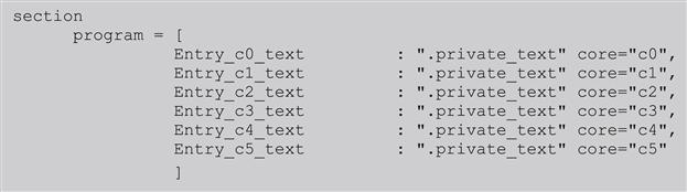
Taking into account the nature of the application, the user specific sections must be placed into dedicated private sections.
In the demo.appli file the definition is implemented as:
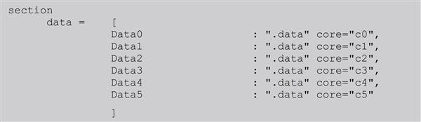
The user specific data must be placed in a private section too. The definition of data sections is done in demo.appli in a similar way as for the code sections:
The last step is to instruct the compiler where to place the default sections generated for the user private code and data.
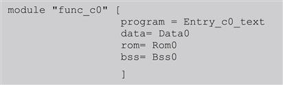
For each user module, the compiler will rename the default sections into the newly created sections like Entry_c0_text, Data0, etc.
After the code is compiled the compiler will export towards the linker the newly created sections offering the user a clear image about the resources that needs to be placed into the appropriate memories. Otherwise, the process would be obfuscated and almost impossible to be handled by users when further changes are required.
The DSP compiler settings are all grouped into a single panel under: Project properties/C/C++ build/Settings as is shown in Figure 17-12.
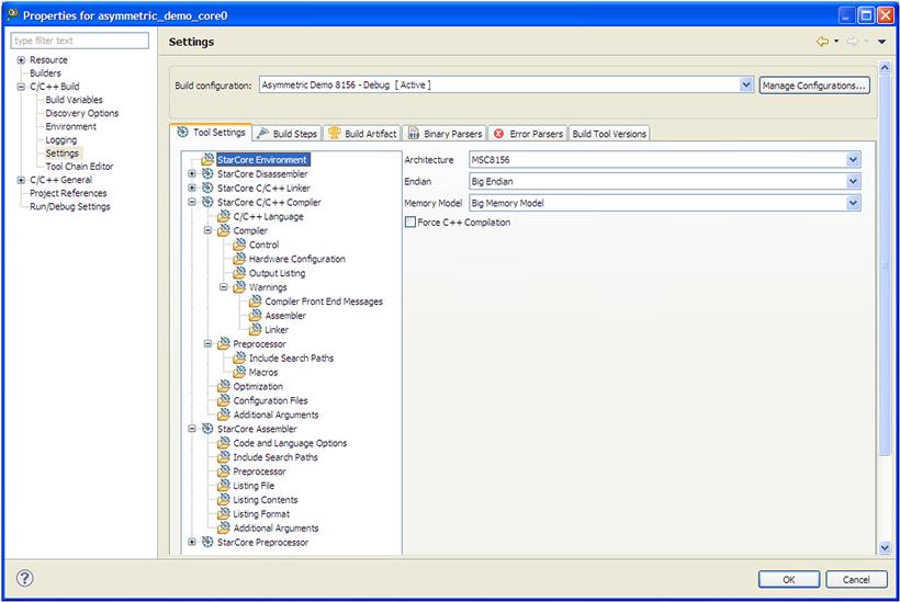
Figure 17-12: DSP compiler settings panel.
The user can control throughout the compiler settings panels how the compiler generates the code, reports the errors and warnings, and how it interacts with the user environments (build steps, make files, output files, logging, etc.).
The external configuration files can be added via the Configuration Files menu as shown in Figure 17-13.
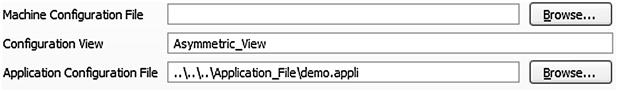
Figure 17-13: Adding custom settings and configuration for DSP compiler.
The DSP compiler offers a wide range of optimizations from the standard C optimization up to the low level target specific optimizations. The user can choose between optimizations for speed or size or can choose to apply cross file optimization techniques (Figure 17-14).

Figure 17-14: Compiler optimization levels.
DSP IDE’s offer an interface that allows advanced users to interfere with compiler internal components and get optimal performance from the code. These options should be used only when the performance is a critical factor.
In order to benefit from the compiler optimization techniques, the user must be able to understand the internal structure of the compiler and how different components and compiler flags/switches and options interact with the user code.
A generic DSP compiler is depicted in Figure 17-15. The user invokes the compiler shell via the DSP IDE by specifying the C sources and assembly files that need to be processed with the appropriate compiler options. The C Front-End indentifies the sources, creates the compilation unit by including all the headers, expands all the macro, and finally converts the file into an intermediate representation which is then passed to the optimizer.
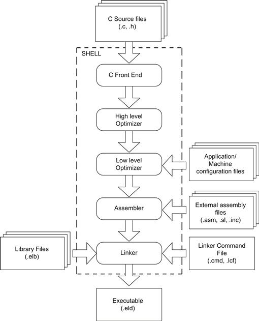
Figure 17-15: Compilation process.
Most of the commercial compilers for DSP have two optimization stages:
• High level optimizer which handles the platform independent optimization stage. Usually, these kinds of optimization are well known and common to most compilers. The optimizations done in this stage consists in: strength reduction (loop transformation), function in-lining, expression elimination, loop invariant code, constant folding and propagation, jump to jump elimination, dead storage and assignment elimination, etc. Also, depending on each vendor compiler technology, the high level optimizer can be instructed to generate specific optimization that includes additional information which is used later on other compiler internal components. At this point, the output is a linear assembly code.
• Low level optimizer which carries out specific target-specific optimizations. It performs instruction scheduling, register allocation, software pipelining, condition execution and prediction, speculative execution, post increment detection, peephole optimization, etc.
The low level optimizer is the most critical internal component, since it differentiates the different compiler technologies. It transforms the linear code into more optimal parallel assembly code. By default, to achieve this step, the low level optimizer uses traditional conservative assumptions.
Advanced users, who have a deep understanding of how the DSP works, can instruct the compiler at this stage to use a more aggressive approach for code optimization and parallelization.
The DSP IDE provides these means via the dedicated GUI as depicted in Figure 17-16.
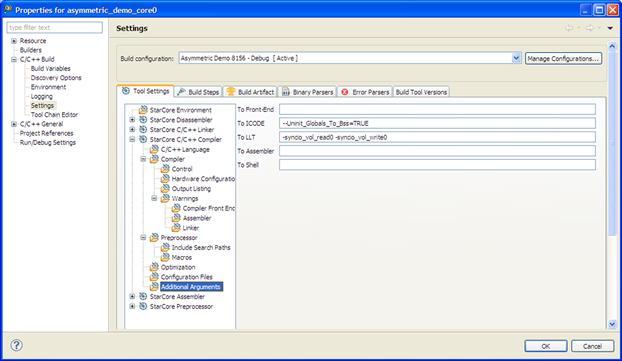
Figure 17-16: Compiler options.
Linker configuration for application
Linking is the last step before getting the executable file. The linker job is to put together all the compiler object files, resolve all the symbols and, based on the allocation scheme, to generate the executable image that will be run on the target.
The DSP linker is based on GNU syntax and it has been enhanced with additional functionalities in order to match the multi-core DSP constraints. The linker is controlled via the linker command files ∗.l3 k.
Most users find the writing of these files to be very difficult. The IDE tries to help such users by providing default physical memory configurations and predefined linker symbols.
The default physical memory is insured by using special designated linker functions such as arch() and number_of_cores(). These kinds of functions instruct the linker to generate the appropriate mapping for the physical memory layout and number of executable files that are needed for the application.
The process of linking all the object files is straightforward once the linker philosophy is correctly understood. In the simplest form the linker requires only three basic steps to correctly map the application:
• Define a virtual memory region where code and data segments need to be placed. This is achieved via the GNU style memory directive:
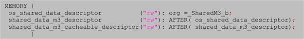
The example above (see theos_msc815x_link.l3 kfrom the asymmetric demo) defines three virtual memory segments called os_shared_data_descriptor, shared_data_m3_descriptor and shared_data_m3_cacheable_descriptor with read and write attribute (e.g. "rw"). The first memory segment os_shared_data_descriptor, starts at the virtual address pointed by the linker symbol _SharedM3_b while the other segments are placed in memory after the end of the previous one.
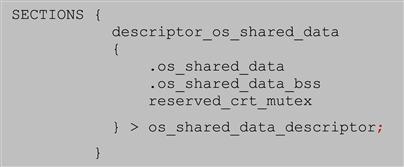
• Assigned the compiler generated output sections into linker output sections and place these sections into the appropriate virtual memory regions defined earlier.
The compiler generated sections such as .os_shared_data are now grouped in a larger linker section called descriptor_os_shared_data that is placed into the virtual memory os_shared_data_descriptor.
• The third step is to map the virtual memory into the physical memory using the address translation table in MMU (memory management unit).
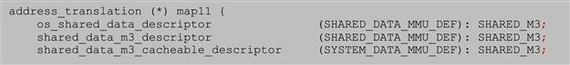
This example maps the virtual memory regions defines earlier over the M3 physical memory (defined here as SHARED_M3) with the MMU attributes SHARED_DATA_MMU_DEF. This symbol is defined in sc3x00_mmu_link_map.l3 k file.
These three basic steps must be duplicated for shared and private memories definitions. In this example, the private code and data for the application that will run independently on each core will look like:
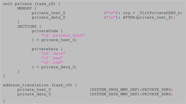
The example shows how the virtual memory for code and data (private_text_0 and private_data_0) are defined and how the compiler sections are then placed and mapped into the proper private physical memory. This code is then duplicated for the rest of the DSP cores.
The last step before linking the application is to add the SDOS library. This is done via the linker Additional Libraries menu as is shown in Figure 17-17.
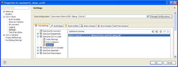
Figure 17-17: Linker additional libraries.
At this point all that remains is to build the project. The DSP IDE by default invokes the GNU Make to build the projects within the workspace. Using makefiles facilitates team work across the network and makes it possible to deploy and build the applications on other operating systems too. The maker settings can be set via the dialogues as shown in Figure 17-18.
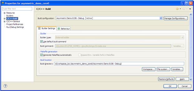
Figure 17-18: Build settings.
When the Project/Build Project option is selected, the IDE based on build settings generates automatically all the intermediate files and starts the building process as shown in Figure 17-19. During the process, the user can visualize, throughout the IDE console, the building progress.
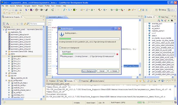
Figure 17-19: DSP application building progress.
Once the building process is finished the user has access to the executable files and can start to debug and instrument the code.
Execute and debug the application on multi-core DSP
The DSP IDE offers a very large set of features for DSP application debugging. The most relevant of them will be discussed in this chapter. As for the C/C++ editing part, the IDE provides a default, fully configurable debug perspective, shown in Figure 17-20.
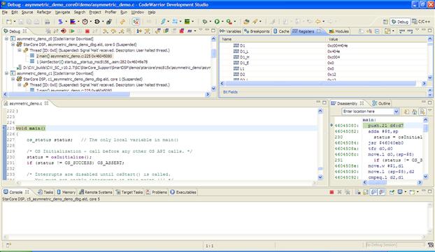
Figure 17-20: IDE defaults debug perspective.
The perspective provides information related to stack frames (upper left corner), variables, registers, cache and breakpoint views (upper right corner), C editor and disassembly (in the middle left and right) and miscellaneous views used for debugging (on lower part of the screen).
Throughout this chapter the main steps and features associated with multi-core debugging will be discussed.
Create a new connection
Before downloading the code to the DSP memory the debugger connection must be defined. The CodeWarrior connection is based on Eclipse Remote System Explorer (RSE) wizard. This allows the user to create a new RSE system that will describe physical connection parameters. Further on, this system can be used to connect different applications with the DSP target without any additional steps.
DSP IDE’s support tree types of connections, depending on the probe used to connect with the target. The physical connections can be done via USBTap or EthernetTap. A third type of connection is done for the simulator and in this case the connect type is CCSSIM2.
To create a new connection system, from the Remote Systems panel select New/Connection. The dialogue window that will appear should be configured as in Figure 17-21.
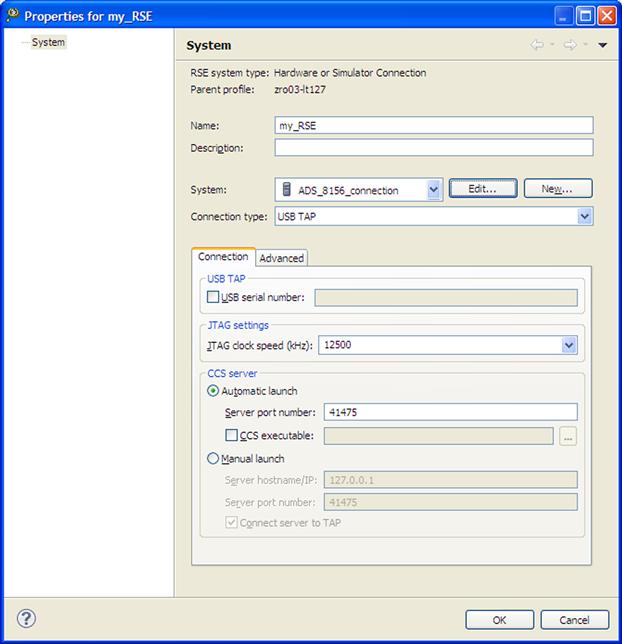
Figure 17-21: RSE system.
Once the connection type and Connection Server (CCS) port is selected the connection is ready. Apart from this basic setup, the CodeWarrior allows users to configure more complex scenarios like remote connection via a remote CCS running on a PC other than the one the DSP IDE is running on.
Also, different JTAG configuration chains and custom debugger memory configurations files and download methods can be selected from system properties (see Figure 17-22).
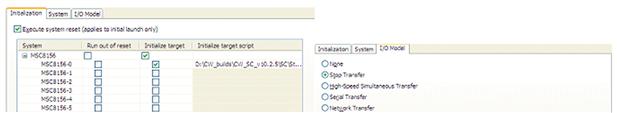
Figure 17-22: Connection properties.
After the connection is correctly configures, the RSE system created (in this case my_RSE) will be visible in the Remote System view and it can be reused in other projects that are built with the same DSP target in mind. The main advantage of this approach is that instead of having for each new project a new connection system, a single system that is kept in the workspace can be utilized for all the projects. If a modification of the RSE system is done, this will be immediately visible and available for all the projects within the workspace.
Set up the launch configuration
Each of the DSP cores must have an associated launch configuration. The launch configuration is an xml file that holds all debugger settings related to a particular executable file. CodeWarrior supports three types of launch configurations:
• Attach launch configuration assumes that code is already running on the board and therefore does not run a target initialization file. The state of the running program is undisturbed. The debugger loads symbolic debugging information for the current build target’s executable.
• Connect launch configuration runs the target initialization file. This file is responsible for setting up the board before connecting to it. The connect launch configuration does not load any symbolic debugging information for the current build target’s executable. Therefore there is no access to source-level debugging and variable display.
• Download launch configuration stops the target, runs an initialization script, downloads the specified executable file, and modifies the program counter.
Depending on the action the user wants to perform, one of these launch configurations can be chosen. The default debug launch configuration for DSP core 0 is shown in Figure 17-23.
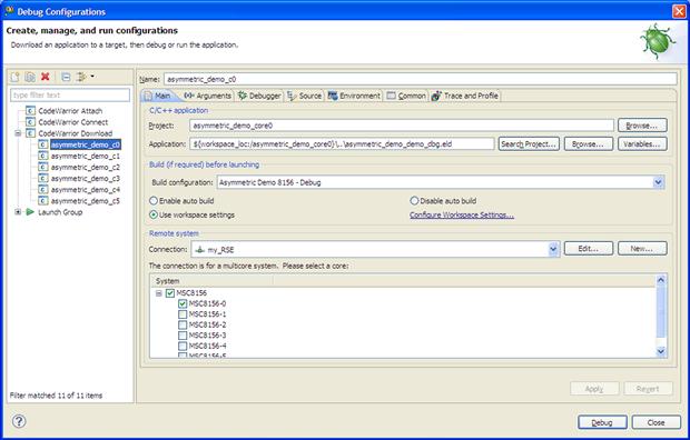
Figure 17-23: Debug launch configuration for DSP core 0.
If more than one executable file must be downloaded to the DSP target, then the Launch Group option can be used to group together two or more launch configurations in a single debugger launch action. When this launch group is executed, the CodeWarrior will automatically load all the executable files and it will make all the appropriate settings with regard to the DSP target. For the asymmetric demo all six debug launch configuration files will be executed as a group (see Figure 17-24).
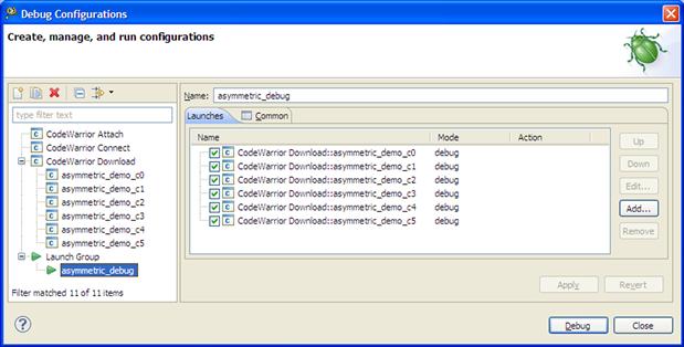
Figure 17-24: Launch group.
Debugger actions
The common debugger actions are listed on top of the Debug panel. Option such as: Reset, Run, Pause, Stop, Disconnect, Step In, Step Over, and Step Out are available for each Debug thread. These options are doubled by their counterpart multi-core options marked with the ‘m’ decorator.
Depending on which debug thread is active, the IDE automatically displays the entire context only for the DSP core that has the debug focus on (Figure 17-25). Moving from one thread to the other the CodeWarrior maintains the correct viewer data coherency. This mechanism is doubled by a caching algorithm whose scope is to reduce the communication with the target and to maintain a flawless fast change between the threads. The target data is read only if the debugger detects a change, otherwise the IDE communication with the target remains idle.

Figure 17-25: Debug threads.
The Register view, shown in Figure 17-26, was enhanced to display all relevant information for the users. Each register that was updated since the last PC change is highlighted and a complete bit-field description for each part of the register is available.
Figure 17-26: Register view.
No debug session can be effectively done without the usage of breakpoints. The IDE supports up to six hardware breakpoints and an unlimited number of software breakpoints. Using simple click actions, the user can install and then inspect the breakpoints in the application. Depending on breakpoint type, the IDE marks the breakpoint with the appropriate decorator as shown in Figure 17-27.
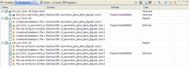
Figure 17-27: Breakpoints view.
Additional information for each breakpoint is displayed. In this case the breakpoints (one HW and two SW) are installed on the same function print_func called from SDOS software timer task. Since this is private to each of the cores, the virtual address is the same for all the cores. The debugger automatically shows on which core the breakpoint was installed. For each breakpoint the user can attach via the Breakpoint Properties menu different actions that can be executed when the breakpoint is hit (see Figure 17-28).
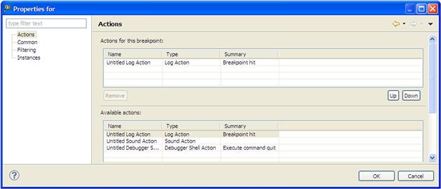
Figure 17-28: Breakpoint actions.
Using the Breakpoint Properties the default behavior of the debugger in case of a breakpoint hit can be changed. A common functionality is conditional breakpoints (see Figure 17-29) what can be used to control breakpoints behavior in case of debugging software loops. The user can instruct the debugger to trigger the breakpoint only when some conditions are met.
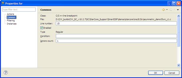
Figure 17-29: Conditional breakpoints.
In the case where a breakpoint is hit or when stepping throughout the code, the debugger highlights the instructions executed and offering a visual trace of executed code as shown in Figure 17-30 where the last three assembly instructions are marked using a gradient color.
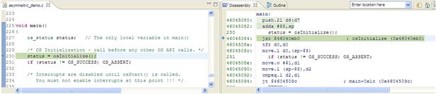
Figure 17-30: Disassembly highlight of the latest executed instructions.
At this point it is very important for a user to understand exactly how a breakpoint interacts with the application and when and how to use a breakpoint in a multicore application.
The hardware breakpoints are implemented by a special processor unit – due to this reason they are limited as number. The logic circuit watches every bus cycle and when a match with the address set for comparison occurs, it then stops the core. The hardware breakpoint does not modify the code, stack, or any target resource, being from this point of view completely non-intrusive.
Even further, it is advisable to use these kinds of breakpoint in a multicore application where the synchronization between threads at run-time is critical. Since these breakpoints do not interact with the program or the core, installation during run time can be done without any negative effects upon the application.
By contrast the software breakpoints always modify the code by inserting a small piece of code (usually the debugger inserts a special instruction that triggers an interrupt when it is executed). From this point of view software breakpoints are intrusive. After the debug interrupt is triggered the debugger stops the core and then replaces the code with the original code.
For DSPs that support variable length instructions sets (VLES) and depending on the type of breakpoint used for debugging, different results might be displayed. On hardware breakpoints case, the debugger stops immediately after the VLES that contains the matched address even if this was at the beginning or middle of the instruction set. Because of this the registers and memory contain the data for the rest of executed instructions within the VLES too.
In case of software breakpoints, the debugger rolls back with one instruction and the content of the registers and memory is actualized with the data before the real instruction execution.
The DPS IDE must provide the tools and method to limit the software breakpoint to the active debug context. Each of the software breakpoints can be set to act on all cores or on a single core. In case the user choose to debug a code section that is shared between multiple cores, then by using the functionality of limited software breakpoints to the active debug context, the debugger will control only core chosen by the user and leaves the other cores to run unaffected. Otherwise, being a shared code section, the debugger will control all the DSP cores.
While a debug session is active, the user can interact with the target via a comprehensive set of features to import or export memory like Memory monitors depicted in Figure 17-31, Target Tasks depicted in Figure 17-32, etc. The import/export memory can be done in various file formats depending on user requirements.
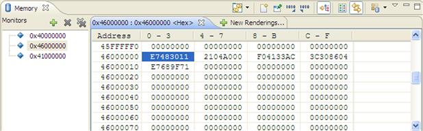
Figure 17-31: Memory view.

Figure 17-32: Target tasks setup.
The IDE provides advance tools for target configuration and verification. For example the MMU configuration tool can be used to inspect the DSP target at any moment during debugging. This is a very useful tool for multi-core applications allowing users to modify on the fly the memory mapping (as is demonstrated in Figure 17-34) or to inspect the source of errors that might appear (as is shown in Figure 17-33 for an illegal memory access due to an initialized pointer).
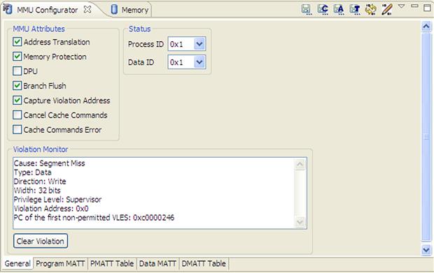
Figure 17-33: MMU general view.
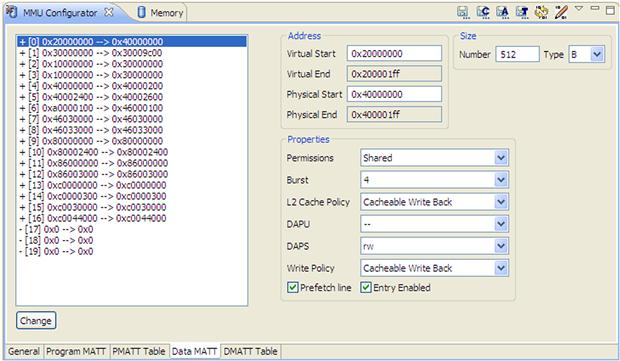
Figure 17-34: MMU data memory translations.
Trace and Profile the multicourse application using hardware and software dedicated resources
Modern DSP systems have a very powerful on-chip Debug and Profiling Unit (DPU) that can be used to monitor and measure the product’s performance, to diagnose errors, and to write trace information of any embedded application that runs on the DSP core. The DPU unit operation is depicted in Figure 17-35.
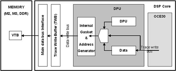
Figure 17-35: DPU workflow.
The DPU writes the trace information that is generated by either itself or the OCE (On Chip Emulator), to a Virtual Trace Buffer (VTB). The VTB can reside in internal or external memory, as specified by the user via the linker command file.
The DPU write accesses are buffered in the Trace Write Buffer (TWB), and then written through the main data bus interface in bursts. The lowest priority bus requests are used when writing into the first unwritten address of the VTB. When the TWB becomes full, it raises the priority of its bus request. At the first cycle after this priority change, the DPU generates a core stall request.
Software Analysis setup
In order to configure and analyze the trace date generated by the DPU, the IDE provides the Software Analysis plug-in.
The DPU setup is done automatically based on few simple options selected by the user as is shown in Figures 17-36 and 17-37.
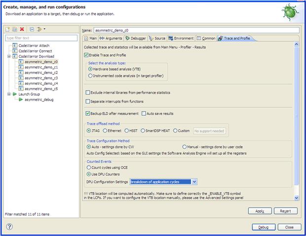
Figure 17-36: Software Analysis main configuration dialogue.
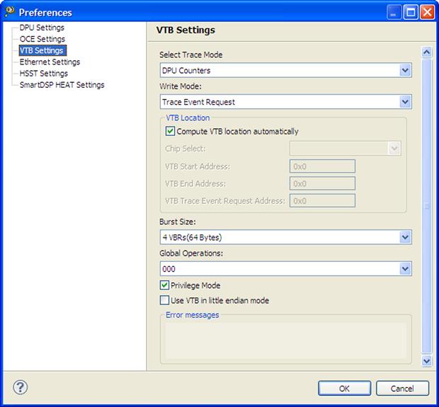
Figure 17-37: VTB settings.
For each of the debug configurations, the user can select to enable the trace. In this way one core or more can be instrumented. From the main configuration dialogue window, the user can select from a wide range of counting events. Using the default options provided by the IDE, the user can configure the DPU to measure the most representative events. Alternatively, the advanced options are available for individual DPU counters setup. Each of the six available counters within the DPU can be configured to measure any DPU supported event.
The VTB location is automatically placed into the appropriate memory via the linker command files. Alternatively the user can choose to place this buffer manually at his discretion into any free memory region on the target. The only constrain regarding the VTB placement is for multi-core application, where due to the nature of data, this buffer must have private privileges for each of the DSP cores. Otherwise the data might be polluted by the other cores events.
Once the VTB is defined at different addresses which do not overlap between the DSP cores, the data management is done automatically by the DPU unit without any additional interaction from the user side.
On the host PC, the DSP IDE handles the data from each VTB separately. In this way, each core can be examined separately from the others.
If the user wants to perform the appropriate DPU settings within the application and wants to utilize the Software Analysis only for results interpretation and display, then the Trace Configuration Method should be set to manual. In this mode, the CodeWarrior will not perform any DPU initializations and will interpret the results based on the DPU registers values found on the target. In this case it is the user’s responsibility to do the correct DPU setup.
Since some applications might dump a lot of trace data into the internal VTB, CodeWarrior provides four methods for downloading the trace from the target to the host. Depending on user hardware and software setup, the CodeWarrior can be instructed to get the trace data via JTAG or Ethernet ports. The fastest method is to use the Ethernet port, but this method requires some additional libraries to be linked with the user application.
The code instrumentation is carried out automatically when a new debug session is launched. The trace results are available immediately when the DSP core is suspended or when the debug session is terminated.
The results for each application are available throughout the associated Trace and Profile Results panel as is shown in Figure 17-38.
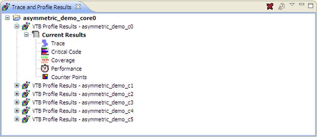
Figure 17-38: Trace and Profile results view.
For each of the debug configurations, there are five submenus available. Each of these submenu display specific analysis that was performed on the generic trace data.
Trace
The Trace submenu shows in the form of a list the raw DPU trace results (see Figure 17-39). It automatically computes and matches the addresses generated by the hardware unit with the executable file symbolic information and appends the corresponding counter values for each pair of events. With the results in this form, the user can perform different actions like exporting the trace or trace filtering in order to find a specific event.
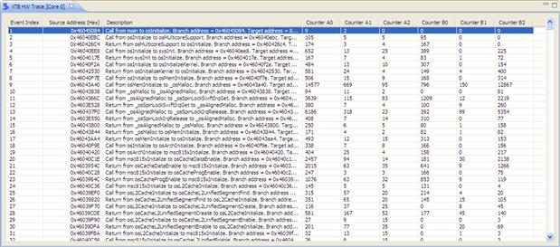
Figure 17-39: Trace results.
Critical code
The Critical code submenu is the most important view of all. It helps the users to optimize the critical part of the applications. For each of the functions within the application, the critical code computes, based on the value of the DPU counters, the number of cycles spent for each block execution as is shown in Figure 17-40.

Figure 17-40: Critical code view.
After the most critical functions have been identified the user can navigate one extra analysis level deep into the code. By selecting the appropriate function, the Critical code will display the instrumentation results for each code line. The viewer can be configured to display the results in different forms (C source only, assembly code only, or mixed).
As shown in Figure 17-41 the user can pinpoint the instructions where most of the processing cycles are spent and then can try to reduce the cycles by taking into account what caused the issue in the first place.
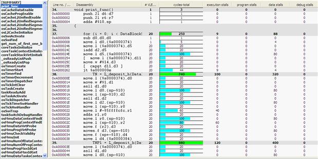
Figure 17-41: Critical code function details level.
For example at line 38, the Critical code shows a high number of data stalls cycles need for DataIn buffer processing. This is a typical case of cache data miss, since the data is not yet in the cache at a time when the processing unit needs it.
Code Coverage
The Code Coverage view compares the actual application trace against the executable file code and produces the mapping of the program counter with the source code. An example is shown in Figure 17-42.
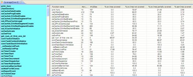
Figure 17-42: Code Coverage summary view.
Usually this feature is used for checking if the algorithm flow is fully covered during the testing phase. Then the PC address found in the raw trace matches the one from the executable file; the code is displayed in green otherwise it is highlighted in magenta. Figures 17-43 and 17-44 show two of these cases of the asymmetric demo. (Please note the printed book does not show the color in these figures.)
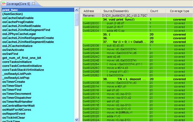
Figure 17-43: Code Coverage function detailed view.
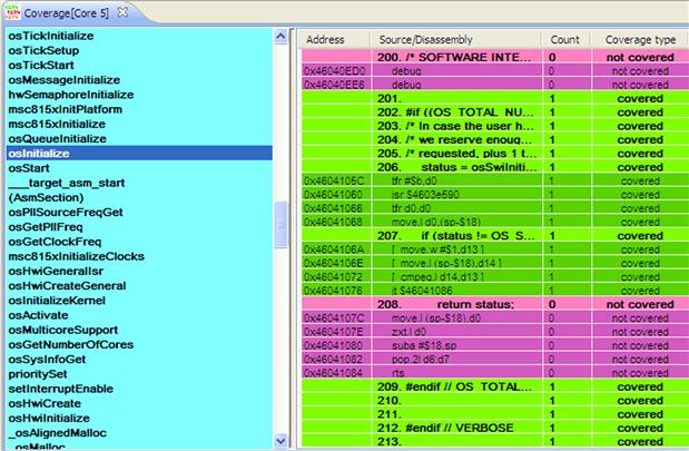
Figure 17-44: Code Coverage details.
If the entire code is highlighted as covered, the user can have the confidence that the tests carried out cover all the possible scenarios that might appear during the application life-time.
Performance
The Software Analysis functions would not be complete without a general summary of the application modules. The mail Performance view provides the application overview and this is demonstrated in Figure 17-45.
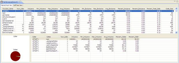
Figure 17-45: Performance statistics.
This view links together all the functions within the application and computes the statistics for both the caller and callee. Based on the raw trace, the IDE computes exactly how many cycles are spend for each function main code (exclusive), or the total cycles measured between a call and return (inclusive). By matching the trace against the executable file the code size can also be computed. In order to help the user to identify the most costly function, the results are aggregated in form of pie that show the overall performance.
The results can be exported direct to Microsoft Excel CSV format. If needed the exported data can be formatted via the Excel in order to meet the user requirements.
Beside the statistics the Performance view assembles the application call tree. The entire map of functions calls for asymmetric demo, shown in Figure 17-46. This feature allows a better understanding of application and operating system flow.
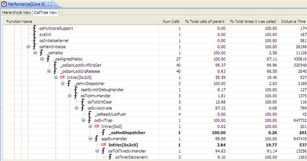
Figure 17-46: Call tree view.