Nondeterministic Events in Mobile Systems
Abstract
This chapter presents essential algorithms that are normally used in mobile robotics for solving the problems of optimum state estimation, sensor data fusion, robot localization, etc. After a short review of probability theory, the basic concepts of Bayesian filtering are introduced. The algorithms are broken down into the basic parts that are studied separately to allow the reader to understand how the algorithm works and to show the influence of the parameters on algorithm performance. The most influential algorithms, Bayesian filter, (extended) Kalman filter, and particle filter, are described in more detail and several simple examples are used to demonstrate the applicability of the algorithms. State estimation algorithms are accompanied with a discussion on observability analysis, estimate convergence, and bias.
Keywords
Probability theory; Stochastic modeling; Bayes’ rule; Observability; Bayesian filter; Kalman filter; Extended Kalman filter; Particle filter
6.1 Introduction
Deterministic events in real world situations are rare. Let us take a look at some examples.
Consider a case where we are measuring the speed of a vehicle. The true speed of the vehicle can never be determined with absolute precision, since the speed sensors have inherent uncertainty (sensitivity, finite resolution, bounded measurement range, physical constraints, etc.). Sensor measurements are susceptible to environmental noise and disturbances, the performance (characteristics) of the sensor normally changes over time, and the sensors sometimes fail or break down. Therefore, the sensors may not provide relevant information about the quantity we are measuring.
Like for sensors, similar conclusions can be drawn for actuators. For example, consider a case of a motor drive. Due to noise, friction, wear, unknown workload, or mechanical failure, the true angular speed cannot be determined based on input excitation.
Furthermore, some algorithms are intrinsically uncertain. Many algorithms are normally designed in a way that produce a result with limited precision (that is satisfactory for a given problem), since the result is required to be obtained in a limited time frame. In mobile robotics, as in many other systems that need to run in real time, the speed of computation is normally more crucial than the absolute precision. Given limited computational resources, real-time implementations of many algorithms with desired response times are not feasible without reduction of algorithm precision.
Moreover, the working environment of mobile agents (wheeled mobile robots) is also inherently uncertain. The uncertainties are normally lower in structured environments (e.g., human-made buildings with planar floors and walls, etc.) and higher in dynamic time-varying environments (e.g., domestic environments, road traffic, human public spaces, forests, etc.).
The development of the autonomous wheeled mobile system must address the problem of uncertainties that are due to various sources.
6.2 Basics of Probability
Let X be a random variable and x be an outcome of the random variable X. If the sample (outcome) space of the random variable X is a set with finite (countable) number of outcomes (e.g., coin tossing has only two possible outcomes, head or tail), X is a discrete random variable. In the case that the sample space is a set of real numbers (e.g., the weight of a coin), X is a continuous random variable. In this section a brief review of basic concepts from probability theory is given. A more involved overview of the topic can be found in many textbooks on statistics (e.g., [1]).
6.2.1 Discrete Random Variable
A discrete random variable X has a finite or countable sample space, which contains all the possible outcomes of the random variable X. The probability that the outcome of a discrete random variable X is equal to x is denoted as
or in a shorter notation P(x) = P(X = x). The range of the probability function P(x) is inside the bounded interval between 0 and 1 for every value in the sample space of X, that is, P(x) ∈ [0, 1] ∀ x ∈ X. The sum of the probabilities of all the possible outcomes of the random variable X is equal to 1:

The probability of two (or more) events occurring together (e.g., random variable X takes value x and random variable Y takes value y) is described by joint probability:
If random variables X and Y are independent, the joint probability (6.2) is simply a product of marginal probabilities:
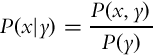
Conditional probability, denoted by P(x|y), gives the probability of random variable X taking the value x if it is a priori known that the random variable Y has value y. If P(y) > 0, then the conditional probability can be obtained from
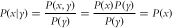
In the case of independent random variables X and Y the relation (6.3) becomes trivial:
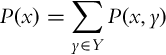
One of the fundamental results in probability theory is the theorem of total probability:
In the case that conditional probability is available, the theorem (6.4) can be given in another form:

In (6.5) the discrete probability distribution was introduced, defined as column vector p(Y ):
where ![]() is the number of all the possible states the random variable Y can take. Similarly, the column vector p(x|Y ) is defined as follows:
is the number of all the possible states the random variable Y can take. Similarly, the column vector p(x|Y ) is defined as follows:
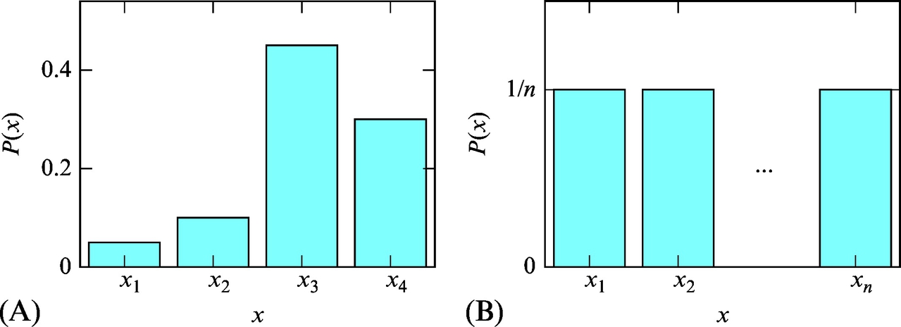
Discrete probability distributions can be visualized with histograms (Fig. 6.1). In accordance with Eq. (6.1), the height of all the columns in a histogram sums to one. When all the states of the random variable are equally plausible, the random variable can be described with a uniform distribution (Fig. 6.1B).
6.2.2 Continuous Random Variable
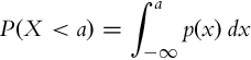
The range of a continuous random variable belongs to an interval (either finite or infinite) of real numbers. In the continuous case, it holds P(X = x) = 0, since the continuous random variable X has an infinite sample space. Therefore a probability density function p(x) is introduced that has a bounded range between 0 and 1, that is, p(x) ∈ [0, 1]. The probability that the outcome of a continuous random variable X is less than a is
Examples of a probability density function are shown in Fig. 6.2. Similarly as Relation (6.1) holds for a discrete random variable, the integral of probability density function over the entire sample space of a continuous random variable X is also equal to one:


Similar relations that hold for a discrete random variable (introduced in Section 6.2.1) can also be extended to a probability density function. Some important relations for discrete and continuous random variables are gathered side-by-side in Table 6.1.
Table 6.1
Selected equations from probability theory for discrete and continuous random variables
| Description | Discrete random variable | Continuous random variable |
| Total probability | ||
| Theorem of total | ||
| probability | ||
| Mean | ||
| Variance |
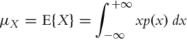
The probability distributions of the random variable are seldom described by various statistics. The mean value of a continuous random variable X is defined as a mathematical expectation:
One of the basic parameters that describe the shape of distribution is variance that is defined as follows:

These properties can also be defined for discrete random variables, and they are given in Table 6.1.
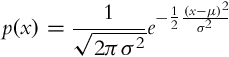
The mean value μ and the variance σ2 are the only two parameters that are required to uniquely describe one of the most important probability density functions, a normal distribution (Fig. 6.3), which is presented with a Gaussian function:
In a multidimensional case, when a random variable is a vector x, the normal distribution takes the following form:
where Σ is the covariance matrix. An example of a 2D Gaussian function is shown in Fig. 6.4. Covariance is a symmetric matrix where the element in the row i and column j is a covariance ![]() between the random variables Xi and Xj.
between the random variables Xi and Xj.


The covariance ![]() is a measure of the linear relationship between random variables X and Y:
is a measure of the linear relationship between random variables X and Y:
where p(x, y) is the joint probability density function of X and Y. The relation (6.9) can be simplified to
If random variables X and Y are independent, then ![]() and the covariance (6.10) is zero:
and the covariance (6.10) is zero: ![]() . However, null covariance does not imply that random variables are independent. Covariance of two identical random variables is the following variance:
. However, null covariance does not imply that random variables are independent. Covariance of two identical random variables is the following variance: ![]() .
.
6.2.3 Bayes’ Rule
Bayes’ rule is one of the fundamental pillars in probabilistic robotics. The definition of Bayes’ rule is
for a continuous space and
for a discrete space. Bayes’ rule normally allows us to calculate the probability that is hard to determine, based on the probabilities that are presumably easier to obtain.
Example 6.1
This is an introductory example of using Bayes’ rule (6.11) in mobile systems. Let a random variable X represent the state of a mobile system that we want to estimate (e.g., a distance of the mobile system from the obstacle) based on the measurement Y that is stochastically dependent on random state X. Since the result of a measurement is uncertain, we would like to know the probability density of the estimated state X = x based on the measurement Y = y.
Solution
We would like to know the probability p(x|y), and this can be calculated from Eq. (6.11). The probability p(x) describes the knowledge about the random variable X before the measurement y is made, and it is therefore known as a priori estimate. The conditional probability p(x|y) gives the knowledge about the random variable X after the measurement is made, and it is therefore also known as a posteriori estimate. The probability p(y|x) contains information about the influence of the state X on the measurement Y, and therefore it represents the model of a sensor (e.g., probability distribution of distance measurement to the obstacle if the mobile system is at specific distance from the obstacle). The probability p(y) contains distribution of the measurement y, that is, the confidence in the measurement. The probability p(y) can be determined using the total probability theorem ![]() . Therefore, the current estimate p(x|y) can be obtained based on a known statistical model of the sensor (i.e., p(y|x)) and a priori estimate p(x).
. Therefore, the current estimate p(x|y) can be obtained based on a known statistical model of the sensor (i.e., p(y|x)) and a priori estimate p(x).
Example 6.2
There are three different paths that all lead to the same goal location. The mobile system picks the first path in 7 out of 10 cases, the second path only in 1 of 10 cases, and the third path in 1 of 5 cases. There is a 5%, 10%, and 8% chance of an obstacle on the first, second, and third paths, respectively.
1. Determine the probability that the mobile system encounters an obstacle when going toward the goal.
2. The mobile system encountered on an obstacle. What is the probability that this happened on the first path?
Solution
Let us denote the first, second, and third path with symbols A1, A2, and A3, respectively, and the obstacle on any path with symbol B. The probabilities of selecting a specific path are the following: P(A1) = 0.7, P(A2) = 0.1, and P(A3) = 0.2. The probability of encountering an obstacle on the first path is P(B|A1) = 0.05, on the second path P(B|A2) = 0.1, and on the third path P(B|A3) = 0.08.
1. The probability that the mobile system encounters an obstacle is
2. The probability that the mobile system gets stuck on the first path can be calculated using Bayes’ rule (6.12):

Using Matlab script shown in Listing 6.1 the probabilities that the mobile robot gets stuck on either of the paths are also calculated.
Example 6.3
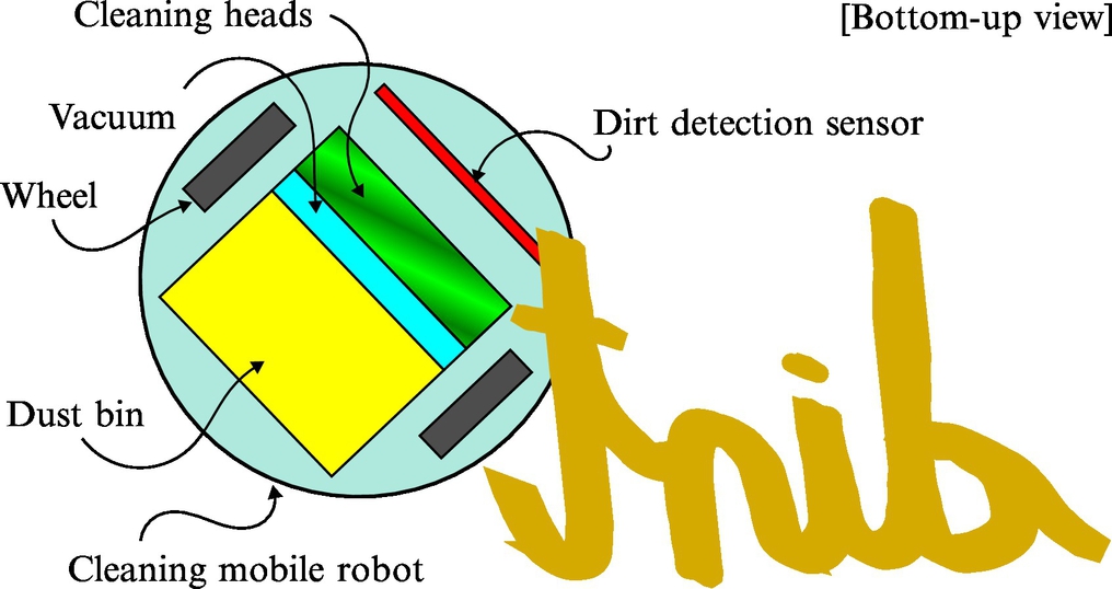
A mobile robot is equipped with a dirt detection sensor that can detect the cleanliness of the floor underneath the mobile robot (Fig. 6.5). Based on the sensor readings we would like to determine whether the floor below the mobile robot is clean or not; therefore, the discrete random state has two possible values. The probability that the floor is clean is 40%. The following statements can be made about the dirt detection sensor: if the floor is clean, the sensor correctly determines the state of the floor as clean in 80%; and if the floor is dirty, the sensor correctly determines the state of the floor as dirty in 90%. The probability of incorrect measurement is small: if the floor is clean, the sensor will incorrectly determine the state of the floor in 1 out of 5 cases, but if the floor is dirty the sensor performance is even better since it makes an incorrect measurement only in 1 out of 10 cases. What is the probability that the floor is clean if the sensor detects the floor to be clean?
Solution
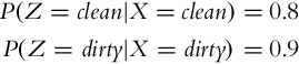
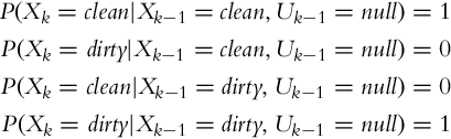
Let us denote the state of the floor with discrete random variable X ∈{clean, dirty} and the measurement of the sensor with random variable Z ∈{clean, dirty}. The probability that the floor is clean can therefore be written as P(X = clean) = 0.4, and the sensor measurement model can be mathematically represented as follows:
Let us introduce a shorter notation:

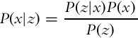
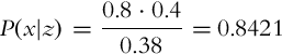
We would like to determine P(x|z) that can be calculated from Bayes’ rule (6.12):
Using the total probability theorem, the probability that the sensor detects floor as clean can be calculated as follows:
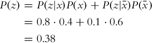
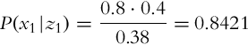
The probability that we are looking for is then
The obtained probability of a clean floor in the case the sensors detect the floor as clean is high. However, there is a more than 15% chance that the floor is actually dirty. Therefore, the mobile system can incorrectly assume that no cleaning is required; and if the mobile robot does not take any cleaning actions, the floor remains dirty.
6.3 State Estimation
In this section an introduction into state estimation is given. State estimation is a process in which the true states of the system are estimated based on the measured data and knowledge about the system. Even if the system states are directly accessible for measurement, the measured data is normally corrupted by noise and other disturbances. This normally makes the raw measured data unsuitable for further use without appropriate signal filtering (e.g., direct use in calculation of control error). In many cases the states of the system may be estimated even if the states are not directly measurable. This can be achieved when the system is said to be observable. When implementing a state estimation algorithm, the system observability should be checked. The most important properties of state estimating algorithms are estimate convergence and estimation bias. This section therefore gives an overview of some practical considerations that should be taken into account before a particular state estimation algorithm is implemented.
6.3.1 Disturbances and Noise
All the system dynamics that are not taken into account in the model of the system, all unmeasurable signals, and modeling errors can be thought of as system disturbances. Under linearity assumption all the disturbances can be presented in a single term n(t) that is added to the true signal y0(t):
Disturbances can be classified into several classes: high-frequency, quasi-stationary stochastic signal (e.g., measurement noise), low-frequency, nonstationary signal (e.g., drift), periodic signal, or some other type of signal (e.g., spikes, data outliers). One of the most important stochastic signals is white noise.
Frequency spectrum and signal distribution are the most important properties that describe a signal. Signal distribution gives the probability that amplitude takes a particular value. Two of the most common signal distributions are uniform distribution and Gaussian (normal) distribution (see Section 6.2). The frequency spectrum of a signal represents the interdependence of a signal in every time moment, which is related to distribution of frequency components composing the signal. In the case of white noise, the distribution of all frequency components is uniform. Therefore the signal value in every time step is independent of the previous signal’s values.
6.3.2 Estimate Convergence and Bias
As already mentioned, the state estimation provides the estimates of internal states based on the measured input-output signals, the relations among the variables (model of the system), and some statistical properties of signals, for example, variances, and other information about the system. All these pieces of information should be somehow fused in order to obtain accurate and precise estimation of internal states. Unfortunately, the measurements, the model, and the a priori known properties of the signals are inherently uncertain due to noises, disturbances, parasitic dynamics, wrong assumptions about the system model, and other sources of error. As a result, the state estimates are in general different from the actual states.
All the above-mentioned problems cause a certain level of uncertainty in signals. Mathematically, the problem can be coped within a stochastic environment where signals are treated as random variables. The signals are then represented by their probability density functions or sometimes simplified by the mean value and the variance. An important issue in a stochastic environment is the quality of a certain state estimate. Especially, the convergence of a state estimate toward the true value has to be analyzed. In particular two important questions should be asked:
1. Is the mathematical expectation of the estimate the same as the true value? If so, the estimate is bias-free. The estimate is consistent if it improves with time (larger observation interval) and it converges to the true value as the interval of observation becomes infinite.
2. Does the variance of the estimation error converge to zero as the observation time approaches infinity? If so and the estimate is consistent, the estimate is consistent in the mean square. This means that with growing observation time the accuracy and the precision of the estimates become excellent (all the estimates are in the vicinity of the true value).
The answers to the above questions are relatively easy to obtain when the assumptions about the system are simple (perfect model of the system, Gaussian noises, etc.). When a more demanding problem is treated, the answers become extremely difficult and analytical solutions are no longer possible. However, what needs to be remembered is that state estimators provide satisfactory results if some important assumptions are not violated. This is why it is extremely important to read the fine print when using a certain state estimation algorithm. Otherwise, these algorithms can provide the estimations that are far from the actual states. And the problem is that we are usually not even aware of this.
6.3.3 Observability
The states that need to be estimated are normally hidden, since information about the states is usually not directly accessible. The states can be estimated based on measurement of the systems’ outputs that are directly or indirectly dependent on system states. Before the estimation algorithm is implemented the following question should be answered: Can the states be estimated uniquely in a finite time based on observation of the system outputs? The answer to this question is related to the observability of the system. If the system is observable, the states can be estimated based on observing the system outputs. The system may only be partially observable; if this is the case, only a subset of system states can be estimated, and the remaining system states may not be estimated. If the system is fully observable, all the states are output connected.
Before we proceed to the definition of observability, the concept of indistinguishable states should be introduced. Consider a general nonlinear system in the following form (![]() ,
, ![]() , and
, and ![]() ):
):
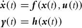
Two states x0 and x1 are indistinguishable if for every admissible input u(t) on a finite time interval t ∈ [t0, t1], identical outputs are obtained [2]:
A set of all indistinguishable states from the state x0 is denoted as ![]() . The definitions of observability can now be given as follows. The system is observable at x0 if a set of indistinguishable states
. The definitions of observability can now be given as follows. The system is observable at x0 if a set of indistinguishable states ![]() contains only the state x0, that is,
contains only the state x0, that is, ![]() . The system is observable if a set of indistinguishable states
. The system is observable if a set of indistinguishable states ![]() contains only the state x for every state x in the domain of definition, that is,
contains only the state x for every state x in the domain of definition, that is, ![]() . Notice that observability does not imply that estimation of x from the observed output may be possible for every input u(t), t ∈ [t0, t1]. Also note that a long time of observation may be required to distinguish between the states. Various forms of observability have been defined [2]: local observability (stronger concept of observability), weak observability (weakened concept of observability), and local weak observability. In the case of autonomous linear systems these various forms of observability are all equivalent.
. Notice that observability does not imply that estimation of x from the observed output may be possible for every input u(t), t ∈ [t0, t1]. Also note that a long time of observation may be required to distinguish between the states. Various forms of observability have been defined [2]: local observability (stronger concept of observability), weak observability (weakened concept of observability), and local weak observability. In the case of autonomous linear systems these various forms of observability are all equivalent.
Checking the observability of a general nonlinear systems (6.14) requires advanced mathematical analysis. The local weak observability of the system can be checked with a simple algebraic test. For this purpose a Lie derivative operator is introduced as the time derivative of h along the system trajectory x:

Consider the system (6.14) is autonomous (u(t) = 0 for every t). To check the local weak observability the system output y needs to be differentiated several times (until the rank of the matrix Q, which is defined later on, increases):
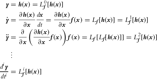
The time derivatives of the system output (6.17) can be arranged into a matrix L(x):
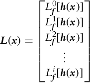
The rank of matrix ![]() determines the local weak observability of the system at x0. If the rank of the matrix Q(x0) is equal to the number of states, that is, rank(Q(x0)) = n, the system is said to satisfy the observability rank condition at x0, and this is a sufficient, but not necessary, condition for local weak observability of the system at x0. If the observability rank condition is satisfied for every x from the domain of definition, the system is locally and weakly observable. A more involved study on the subject of observability can be found in, for example, [2–4].
determines the local weak observability of the system at x0. If the rank of the matrix Q(x0) is equal to the number of states, that is, rank(Q(x0)) = n, the system is said to satisfy the observability rank condition at x0, and this is a sufficient, but not necessary, condition for local weak observability of the system at x0. If the observability rank condition is satisfied for every x from the domain of definition, the system is locally and weakly observable. A more involved study on the subject of observability can be found in, for example, [2–4].
The observability rank condition simplifies for time-invariant linear systems. For a system with n states in the form ![]() , y(t) = Cx(t) the Lie derivatives in Eq. (6.18) are
, y(t) = Cx(t) the Lie derivatives in Eq. (6.18) are
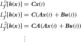
Partial differentiation of Lie derivatives (Eq. 6.19) leads to the Kalman observability matrix Q:
The system is observable if the rank of the observability matrix has n independent rows, that is, the rank of the observability matrix equals the number of states:
6.4 Bayesian Filter
6.4.1 Markov Chains
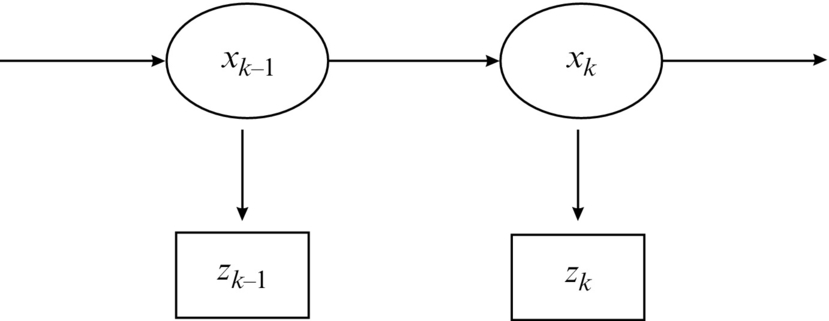
Let us focus on systems for which a proposition about a complete state can be assumed. This means that all the information about the system in any given time can be determined from the system states. The system can be described based on the current states, which is a property of the Markov process. In Fig. 6.6, a hidden Markov process (chain) is shown where the states are not accessible directly and can only be estimated from measurements that are stochastically dependent on the current values of the states. Under these assumptions (Markov process), the current state of the system is dependent only on the previous state and not the entire history of the states:
Similarly, the measurement is also assumed to be independent of the entire history of system states if only the current state is known:
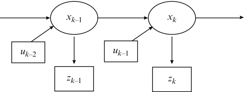
The structure of a hidden Markov process where the current state xk is dependent not only on the previous state xk−1 but also on the system input uk−1 is shown in Fig. 6.7. The input uk−1 is the most recent external action that influences the internal states from time step k − 1 to the current time step k.
6.4.2 State Estimation From Observations
A Bayesian filter is the most general form of an algorithm for calculation of probability distribution. A Bayesian filter is a powerful statistical tool that can be used for location (system state) estimation in the presence of system and measurement uncertainties [5].
The probability distribution of the state after measurement (p(x|z)) can be estimated if the statistical model of the sensor p(z|x) (probability distribution of the measurement given a known state) and the probability distribution of the measurement p(z) are known. This was shown in Example 6.3 for a discrete random variable.
Let us now take a look at the case of estimating the state x when multiple measurements z are obtained in a sequence. We would like to estimate p(xk|z1, …, zk), that is, the probability distribution of the state x in time step k while considering the sequence of all the measurements until the current time step. The Bayesian formula can be written in a recursive form:
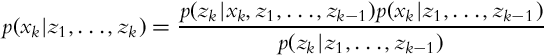
that can be rewritten into a shorter form:
The meanings of the terms in Eq. (6.22) are as follows:
• p(xk|z1:k) is the estimated state probability distribution in time step k, updated with measurement data.
• p(zk|xk, z1:k−1) is the measurement probability distribution in time step k if the current state xk and previous measurements up to time k − 1 are known.
• p(xk|z1:k−1) is the predicted state probability distribution based on previous measurements.
• p(zk|z1:k−1) is the measurement probability (confidence in measurement) in time step k.
Normally it holds that the current measurement zk in Eq. (6.22) is independent on the previous measurements z1:k−1 (complete state assumption, Markov process) if the system state xk is known:
Therefore, Eq. (6.22) simplifies into the following:
The derivation of Eq. (6.23) is given in Example 6.4.
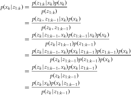
Example 6.4
As an exercise, derive Eq. (6.23) from Eq. (6.22) if the complete state assumption is taken into account (p(zk|xk, z1:k−1) = p(zk|xk)).
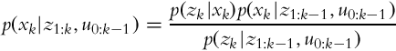
The recursive formula (6.23), which updates the state based on previous measurements, contains a prediction term p(xk|z1:k−1). The state estimation can be separated into two steps: a prediction step and a correction step.
Prediction Step
The prediction p(xk|z1:k−1) is made as follows:
The complete state assumption yields a simpler form:
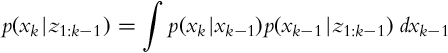
where p(xk|xk−1) represents probability distribution of state transitions and p(xk−1|z1:k−1) is the corrected probability distribution of the estimated state from the previous time step.
Correction Step
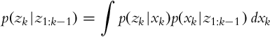
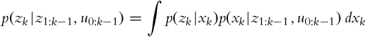
The estimated state probability distribution after the measurement in time step k and predicted state probability distribution in the prediction step are known as the following:
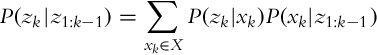
The probability p(zk|z1:k−1) that describes the measurement confidence can be determined from the relation
The Most Probable State Estimate
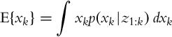
How can the estimated probability density distribution p(xk|z1:k) be used in calculation of the most probable state xk? The best and most probable state estimate (mathematical expectation) ![]() is defined as the value that minimizes the average square error of the measurement:
is defined as the value that minimizes the average square error of the measurement:
Moreover, the value of ![]() , which maximizes the posterior probability p(xk|z1:k), can also be estimated:
, which maximizes the posterior probability p(xk|z1:k), can also be estimated:
Example 6.5
Consider Example 6.3 again and determine the probability that the floor is clean if the sensor in time step k = 2 again detects the floor to be clean.
Solution
In time step k = 1 of Example 6.3 the following situation was considered: the floor was clean and the sensor also detected the floor to be clean (z1 = clean). The following conditional probability was calculated:
In the next time step k = 2 the sensor returns a reading z2 = clean with probability P(z2|x2) = 0.8 of a correct sensor reading and with probability ![]() of an incorrect sensor reading (the sensor characteristic was assumed to be time invariant).
of an incorrect sensor reading (the sensor characteristic was assumed to be time invariant).
Let us first evaluate the predicted probability P(x2|z1), that is, the floor is dirty based on the previous measurement. Considering Eq. (6.24), where the operation of integration is substituted for the operation of summation, yields

For now assume that the mobile system only detects the state of the floor, but it cannot influence the state of the floor (i.e., the mobile system does not perform any floor cleaning and also cannot make the floor dirty). Therefore, the state transition probability is simply P(x2|x1) = 1 and ![]() . Hence,
. Hence,
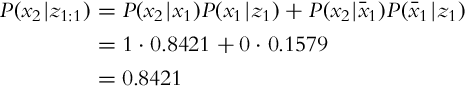
which is a logical result since if the measurement z2 is not considered, no new information about the system has been obtained. Therefore, the state of the floor has the same probability in the time step k = 2 as it was the state probability in the previous time step k = 1.
The measurement can be fused with the current estimate in the correction step, using relation (6.25):
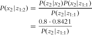
where the value of the normalization factor needs to be calculated. The missing factor is the probability of a clean floor in time step k = 2, and it can be determined with the summation of all the possible state combinations that result in the current measurement zk, considering the outcomes of the previous measurements z1:k−1:
In our case,
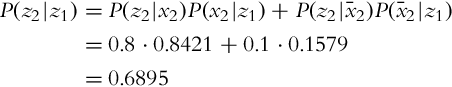
The final result, the probability that the floor is clean if the sensor has detected the floor to be clean twice in a row, is
Example 6.6
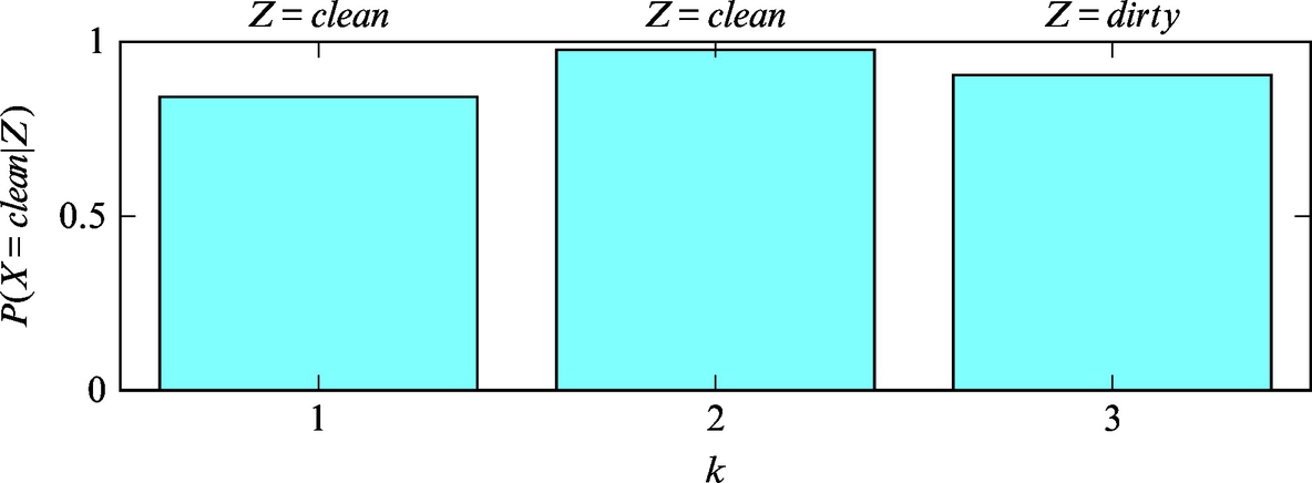
Again consider Example 6.3 and determine how the state probability changes if the floor is clean and the sensor makes three measurements z1:3 = (clean, clean, dirty).
Solution
The first two conditional probabilities were already calculated in Examples 6.3 and 6.5, the third is
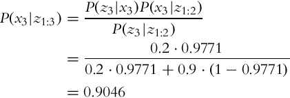
where P(Z = dirty|X = clean) = 1 − P(Z = clean|X = clean). The state probabilities in three consequential state measurements taken at time steps i = 1, 2, 3 are therefore
The posterior state probability distribution for time steps k = 1, 2, 3 is also shown in Fig. 6.8. Implementation of the solution in Matlab is shown in Listing 6.2.
6.4.3 State Estimation From Observations and Actions
In Section 6.4.2 the state of the system was estimated based only on observing the environment. Normally the actions of the mobile system can have an effect on the environment; therefore, the system states can change due the mobile system actions (e.g., the mobile system moves, performs cleaning actions, etc.). Every action that the mobile system makes has an inherent uncertainty. Therefore, the outcome of the action is not deterministic, but it has an inherent uncertainty (probability). The probability p(xk|xk−1, uk−1) describes the probability of transition from the previous state into the next state given a known action. The action uk−1 takes place in time step k − 1 and is active until time step k. Therefore, this action is also known as the most recent or current action. In a general case, the actions that take place in the environment increase the level of uncertainty about our knowledge of the environment, and the measurements made in the environment normally decrease the level of uncertainty.
Let us take a look at what effects the actions and measurements have on our knowledge about the states. We would like to determine the probability p(xk|z1:k, u0:k−1), where z indicates the measurements and u indicates the actions.
As in Section 6.4.2, the Bayesian theorem can be written as follows:

where the following applies:
• p(xk|z1:k, u0:k−1) is the estimated state probability distribution in time step k, updated with measurement data and known actions.
• p(zk|xk, z1:k−1, u0:k−1) is the measurement probability distribution in time step k, if the current state xk, previous actions and measurements up to time step k − 1 are known.
• p(xk|z1:k−1, u0:k−1) is the predicted state probability distribution based on previous measurements and actions made up to time step k.
• p(zk|z1:k−1, u0:k−1) is the measurement probability (confidence in measurement) in time step k.
Note that action indices are in the range from 0 to k − 1, since the actions in the previous time steps influence the behavior of the system states in step k.
Furthermore, the current measurement zk in Eq. (6.26) can be described only with system state xk, since the previous measurements and actions do not give any additional information about the system (complete state assumption, Markov process):
Hence, the relation (6.26) can be simplified:
The recursive rule (6.27), update of the state-probability estimate based on the previous measurements and actions, also includes prediction p(xk|z1:k−1, u0:k−1), where the probability distribution for state estimate is made based on previous measurements z1:k−1 and all the actions u0:k−1. Therefore, the state estimation procedure can be split into a prediction step and a correction step. In the prediction step the latest measurement is not known yet, but the most recent action is known. Therefore, the state probability distribution can be estimated based on the system model. When the new measurement is available, the correction step can be made.
Prediction Step
The prediction p(xk|z1:k−1, u0:k−1) can be evaluated using the total probability theorem:

where due to the complete state the following assumption holds:
Moreover, the most recent action uk−1 is not required for a state estimate in the previous time step:
This yields the final form of the prediction step:

where p(xk|xk−1, uk−1) is the state transition probability distribution and p(xk−1|z1:k−1, u0:k−2) is the corrected state probability distribution from the previous time step.
Correction Step
The state estimate when the measurement in time step k is available and previously calculated prediction is then as follows:
The probability p(zk|z1:k−1, u0:k−1) that represents the confidence in the measurement is the following:
General Algorithm for a Bayesian Filter
The general form of the Bayesian algorithm is given as a pseudo code in Algorithm 3. The conditional probability of the correction step p(xk|z1:k, u0:k−1), which gives the state probability distribution estimate based on known actions and measurements, is also known as belief, and it is normally denoted as
The conditional probability of the prediction p(xk|z1:k−1, u0:k−1) is therefore normally denoted as

The Bayesian filter is estimating the probability distribution of the state estimate. In a moment, when the information about the current action uk−1 is known, the prediction step can be made, and when the new measurement is available, the correction step can be made. Let us introduce the normalization factor ![]() . The Bayesian filter algorithm (Algorithm 3) first calculates the prediction and then the correction that is properly normed.
. The Bayesian filter algorithm (Algorithm 3) first calculates the prediction and then the correction that is properly normed.
As it can be observed from Algorithm 3, an integral must be evaluated to determine the probability distribution in the prediction step. Hence the implementation of the Bayesian algorithm is limited to simple continuous cases, where an explicit integral solution can be determined, and discrete cases with countable number of states, where the operation of integration can be substituted for the operation of summation.
Example 6.7
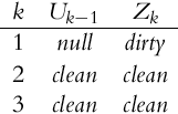
A mobile robot is equipped with a sensor that can detect if the floor is clean or not (Z ∈{clean, dirty}). The mobile system is also equipped with a cleaning system (a set of brushes, a vacuum pump, and a dust bin) that can clean the floor, but the cleaning system is engaged only if the robot believes the floor needs cleaning (U ∈{clean, null}). Again we would like to determine if the floor is clean or not (X ∈{clean, dirty}).
The initial probability (belief) that the floor is clean is
The correctness of the sensor measurements is given with a statistical model of the sensor:

The outcome probabilities if the robot decides to perform floor cleaning are the following:

If the cleaning system is not activated, the following outcome probabilities can be assumed:
Assume that the mobile system first makes an action and then receives the measurement data. Determine the belief belp(xk) based on the action taken (prediction) and the belief bel(xk) based on measurement bel(xk) (correction) for the following sequence of actions and measurements:
Solution
Without loss of generality let us introduce the following notation: Xk ∈{clean, dirty} as ![]() , Zk ∈{clean, dirty} as
, Zk ∈{clean, dirty} as ![]() , and Uk ∈ (clean, null) as
, and Uk ∈ (clean, null) as ![]() .
.
Let us use Algorithm 3. In time step k = 1, when the action ![]() is active we can determine the predicted belief that the floor is clean is the following:
is active we can determine the predicted belief that the floor is clean is the following:
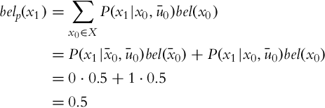
and the predicted belief that the floor is dirty:

Since no action has been taken, the state probabilities are unchanged. Based on the measurement ![]() the belief can be corrected:
the belief can be corrected:
and
After the normalization factor η is evaluated:

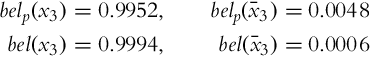
The final values of the belief can be determined:
The procedure can be repeated for time step k = 2, where u1 = clean and z2 = clean:
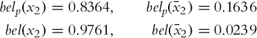
And it can be continued for time step k = 3, where u2 = clean and z3 = clean:
The solution of Example 6.7 in Matlab is given in Listing 6.3.
6.4.4 Localization Example
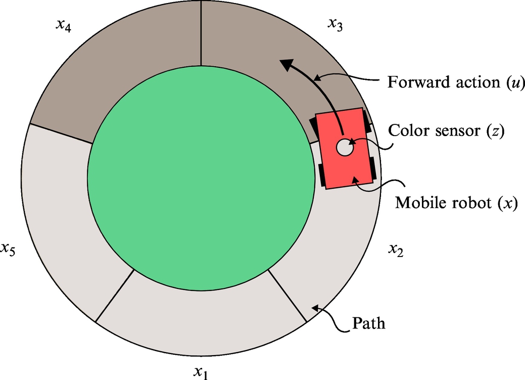
A simple example will be used for presentation of the localization principle that presents the basic idea behind the Monte Carlo localization algorithm. Consider a mobile system that moves in an environment and has a capability of environment sensing. Based on the information from sensor readings and applied movement actions, the localization algorithm should determine the pose of the mobile system in the environment. To implement the localization algorithm the total probability theorem and Bayes’ rule are used, and they represent the fundamental part in the Bayesian filter. In the following sections, the process of measurement in the presence of sensor uncertainties is presented, followed by the process of action in the presence of actuator uncertainties. The mobile system makes actions to change the state of the environment (the mobile system pose changes as the mobile system moves).
Example 6.8
Consider a round path on which the mobile system can move in a forward or backward direction. The path is made out of a countable number of bright and dark tiles in some random order, where the width of a tile matches the width of the path. The mobile system can be positioned on any of the tiles that are marked with numbers. Without loss of generality, consider that the path consists of five tiles as shown in Fig. 6.9. Every tile presents a cell in which the mobile system can be positioned; therefore, this is a discrete representation of the environment. The mobile system knows the map of the environment (the sequence of bright and dark tiles is known), but it does not know which cell it is occupying. The initial belief of mobile system position is therefore given with a uniform distribution, since every cell has equal probability. The mobile system has a sensor for detection of bright and dark tiles, but the sensor measurements are uncertain. The mobile system has an implemented capability for moving for desired number of tiles in a forward or backward direction, but the movement is inherently uncertain (the mobile system can move too little or too much). This sample case will be used in the explanation of the basic concept of the process of environment detection and the process of movement in the environment.