Path Planning
Abstract
This chapter defines path planning, lists possible fields of use, and states some additional terms that need to be met in the process of planning. Several possible ways to describe a planning problem and environment for the later path planning are given, such as graph representations, decomposition to cells, roadmaps, potential fields, and sampling-based path planning. Most commonly used search algorithms in path planning are described, starting with simple bug algorithms and continue with more advanced algorithms that can guarantee the optimal path and can include heuristics to narrow the search area or guarantee completeness. Also, some algorithms that do not require a fully known environment are introduced. For better understanding several illustrating examples and some implementations in Matlab scripts are given.
Keywords
Path planning; Configuration space; Graph presentations; Road map; Optimal search; Heuristic algorithms; Bug algorithms; Randomized algorithms
4.1 Introduction
Path planning from location A to location B, simultaneous obstacle, avoidance and reacting to environment changes are simple tasks for humans but not so straightforward for an autonomous vehicle. These tasks present challenges that each wheeled mobile robot needs to overcome to become autonomous. A robot uses sensors to perceive the environment (up to some degree of uncertainty) and to build or update its environment map. In order to determine appropriate motion actions that lead to the desired goal location, it can use different decision and planning algorithms. In the process of path planning, the robot’s kinematic and dynamic constraints should be considered.
Path planning is used to solve problems in different fields, from simple spatial route planning to selection of an appropriate action sequence that is required to reach a certain goal. Since the environment is not always known in advance, this type of planning is often limited to the environments designed in advance and environments that we can describe accurately enough before the planning process. Path planning can be used in fully known or partly known environments, as well as in entirely unknown environments where sensed information defines the desired robot motion.
Path planning in known environments is an active research area and presents a foundation for more complex cases where the environment is not known a priori. This chapter presents an overview of the most often used path planning approaches applicable to wheeled mobile robots. First, some basic definitions of path planning are given. For more detailed information and further reading see also [1–3].
4.1.1 Robot Environment
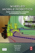
The environment in which the robot moves consists of free space and space occupied by the obstacles (Fig. 4.1). The start and goal configuration are located in free space. Configuration is a complete set of parameters that define the robot in space. These parameters usually include robot position and orientation or also its joints angles. The number of these parameters equals to the number of degrees of freedom (DOF).

The environment that includes moving obstacles is the dynamic environment, while the static environment does not change with time. The environment with known positions of the obstacles is called known the environment; otherwise, the environment is unknown.
4.1.2 Path Planning
Path planning is the task of finding a continuous path that will drive the robot from the start to the goal configuration. The entire path must lie in the free space (as shown in Fig. 4.1). In path planning the mobile system uses known environment map, which is stored in the robot’s memory.
The state or configuration gives a possible pose of the robot in the environment, and it can be represented as a point in the configuration space that includes all possible robot states (configurations). The robot can move from one state to the other by implementing different actions. A suitable path is therefore described as a sequence of actions that guide the robot from the start configuration (state) through some intermediate configurations to the goal configuration. Which action is chosen in the current state and which state will be next depends on the used path planning algorithm and used criteria. The algorithm chooses the next most suitable state from the set of all possible states that can be visited from the current state. This decision is made according to some criteria function, usually defined with one of the distance measures, such as the shortest Euclidean distance to the goal state.
Between certain start and goal states, there may be one or more paths, or there is no path at all that connects the states. Usually there are several feasible paths (i.e., paths that do not collide with obstacles). To narrow the selection choice additional demands or criteria are introduced that define desired optimality:
• the path length must be the shortest,
• the suitable path is the one in which the robot can pass in the shortest time,
• the path should be as far as possible from the obstacles,
• the path must be smooth without sharp turns,
• the path must consider motion constraints (e.g., nonholonomic constraints, where at the current time not all driving directions are possible).
4.1.3 Configuration and Configuration Space
Configuration is the state of the system in the environment space spanned in n dimensions. The state vector is described by q = [q1, …, qn]T. The state q is a point in n-dimensional space called configuration space Q, which presents all possible configurations of the mobile system according to its kinematic model.
Part of the configuration space that is occupied by the obstacles Oi is denoted ![]() . So the free part of the environment without the obstacles is defined by
. So the free part of the environment without the obstacles is defined by
Qfree therefore contains space where the mobile system can plan its motion.
Assume there is a circular robot that can only execute translatory motions in a plane (i.e., it has two DOF q = [x, y]T) then its configuration can be defined by a point (x, y) presenting the robot center. In this case the configuration space Q is determined by moving the robot around obstacles while keeping it in contact with the obstacle, as shown in Fig. 4.2. In doing so the robot center point describes the border between Qfree and Qobs. In other words, the obstacles are enlarged by the known robot dimension (radius) in order to treat the robot as a point in the path planning problem.
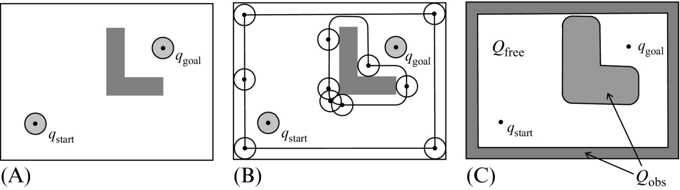
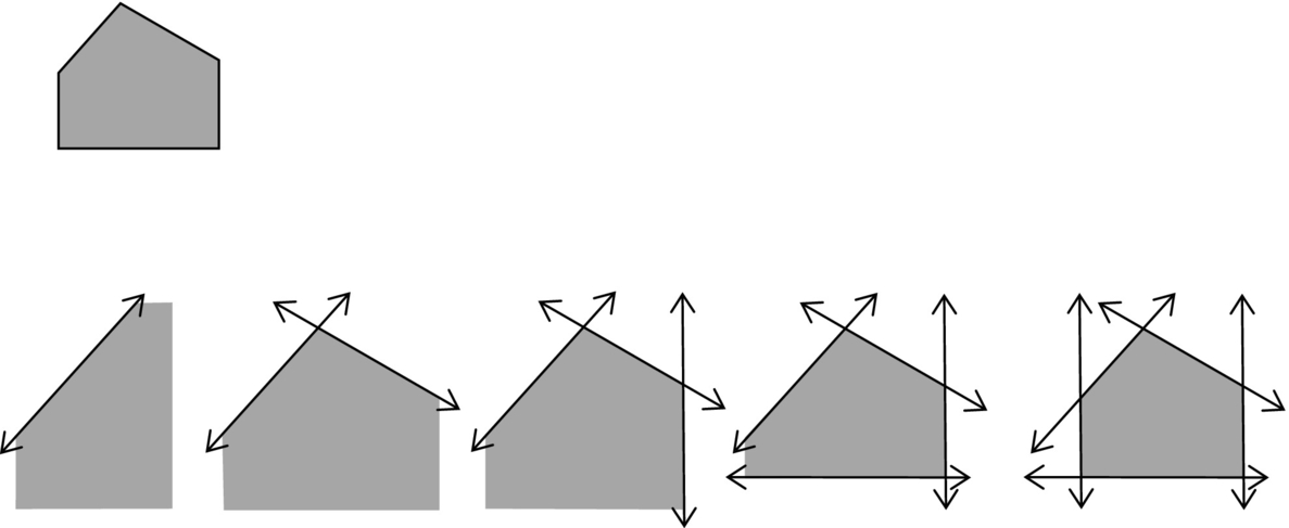
An additional example of configuration space for a triangular robot and rectangular obstacle is shown in Fig. 4.3. The robot can only move in x and y directions (q = [x, y]T).
If the robot from Fig. 4.3 could also rotate then its configuration would have three dimensions q = [x, y, φ]T and the configuration space would be more complex. By simplification we could determine the configuration space using a circle that outlines the robot shape and has a center in the robot center. Obtained configuration Qfree is then smaller than the true free configuration because the outlined circle area is bigger than the robot area. However, this significantly simplifies the path planning problem.
4.1.4 Mathematical Description of Obstacle Shape and Pose in the Environment
The mathematical description of obstacle shape and position is required to estimate robot configuration space and additional environment simplifications. The two most common approaches to describe the obstacles are border presentation by recording vertices and presentation given with half-planes.
Border-Based Description of Obstacles
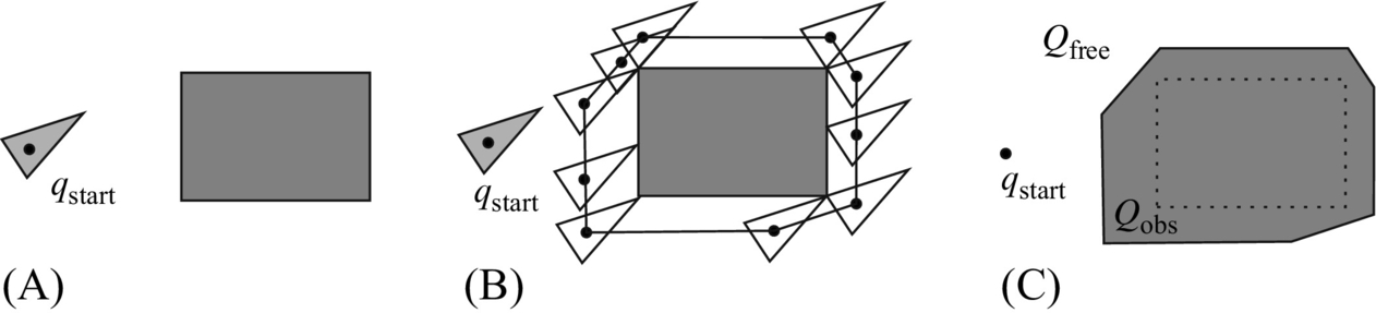
The obstacle ground plan is an m-sided polygon and has m vertices. The obstacle border (shape) can be described by its vertices that are listed in counterclockwise order. The holes in the obstacles and surrounding walls are described by vertices in the clockwise order (Fig. 4.4). Such an obstacle description is valid for convex and nonconvex polygons.
Obstacle Description Using Intersecting Half-Planes
A convex polygon with m vertices can be described by a union of m half planes, where the half plane is defined as f(x, y) ≤ 0 for straight lines or f(x, y, z) ≤ 0 for planes (3D obstacles). An example of how to describe a polygon with five vertices is given in Fig. 4.5. Nonconvex shapes or shapes with holes can be described with the use of operations over sets such as union, intersections, difference among sets, and the like.
4.2 Environment Presentation for Path Planning Purposes
Before path planning, the environment needs to be presented in a unified mathematical manner that is suitable for processing in path searching algorithms.
4.2.1 Graph Representation
Configuration space consists of free space, which contains all possible configurations (states) of the mobile system, and space occupied by obstacles. If free space is reduced and presented by a subset of configurations (e.g., centers of cells) that include start and goal configurations, the desired number of intermediate configurations and transitions among them, then the state transition graph (also graph) is obtained. States are presented by circles and called nodes, and connections among them are given by lines. The connections (lines) therefore present actions required for the system to move among the states.
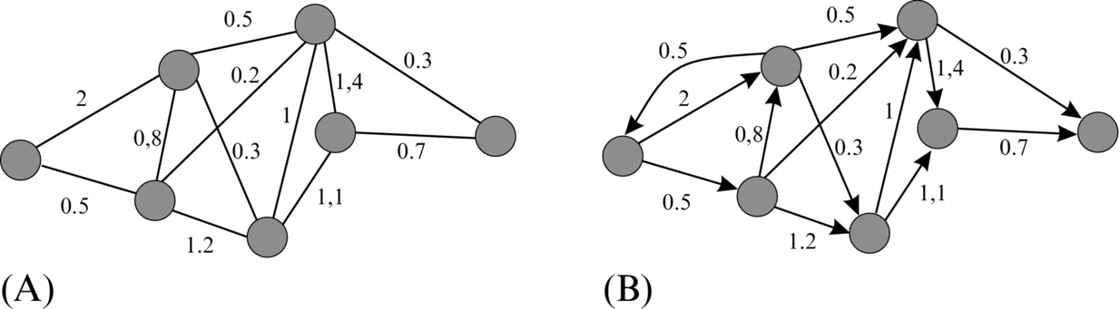
In a weighted graph each connection has some prescribed weight or cost that is needed for action execution and transition among the states of this connection. In a directed graph the connections are also marked with possible directions. In a directed graph the cost depends on the direction of transition, while in an undirected graph the transition is possible in both directions. Fig. 4.6 shows an example of a weighed and directed weighted graph. Path searching in a graph is possible with different algorithms such as A⋆, Dijkstra’s algorithm, and the like.
4.2.2 Cell Decomposition
The environment can be partitioned to cells, which are usually defined as simple geometric shapes. Cells must be convex because each straight line segment connecting any two configurations inside the cell must lie entirely in that cell. An environment partitioned to cells can be presented with a state transition graph where states are certain points inside the cells (e.g., centers) and connections among the states (nodes) are possible only between neighbor cells (e.g., the ones with a common edge).
Accurate Decomposition to Cells
Decomposition to cells is accurate if all the cells lie entirely in the free space or entirely in the space occupied by the obstacles. Accurate decomposition is therefore without losses because the union of all free cells equals the free configuration space Qfree.
An example of accurate decomposition to cells is vertical decomposition, shown in Fig. 4.7. This decomposition can be obtained by using an imaginary vertical line traveling from the left environment border to the right border. Whenever an obstacle corner appears (vertices of some polygon) a vertical border between the cells is made, traveling from the corner only up or only down, or up and down. The complexity of this approach depends on the geometry of the environment. For simple environments the number of cells and the connection among them is small; while with the increasing number of polygons (obstacles) and their vertices, the number of cells also increases.
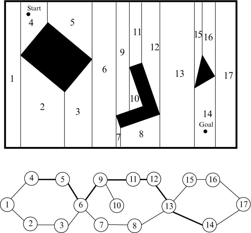
Accurate decomposition to cells can be presented with a state transition graph where graph nodes are, for example, the cells’ centers and the transitions among the cells go, for example, through the middle points of the borders between the cells.
Approximate Decomposition to Cells
Environment decomposition to cells is approximate when it is possible that certain cells contain free configuration space as well as an obstacle or only part of some obstacle. All cells containing at least part of the obstacle are therefore normally marked as occupied, while the remaining cells are marked as free. If decomposition to the cells is made of the same size, then an occupancy grid (Fig. 4.8) is obtained.

The center of each cell (in Fig. 4.8, the free cell is marked with white) is presented as a node in a graph. Transitions among the cells are in four or eight directions if diagonal transitions are allowed. This approach is very simple for application, but due to the constant cell size some information about the environment might get lost (this is not lossless decomposition); for example, obstacles are enlarged and narrow passages among them might get lost. The main drawback of this approach is the memory usage, which increases either by enlarging the size of the environment or by lowering the cell size.
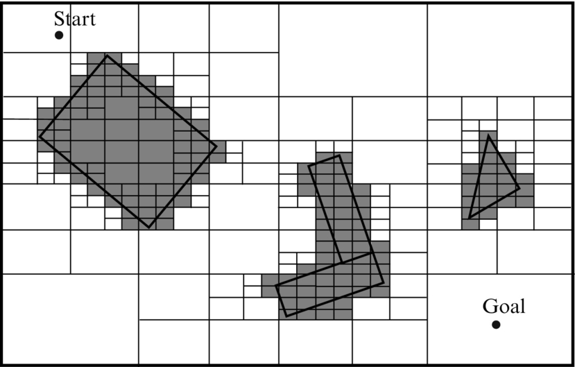
A smaller loss of the environment information at lower memory usage is obtained if the variable cells size is used. A representative example of the latter are quadtrees where initially a single cell is put over the environment. If entire cell is in free space or the entire cell is occupied by the obstacle then the cell remains as is. Otherwise, if this cell is only partly occupied by an obstacle, then it is split into smaller cells. This procedure is repeated until there is a desired resolution. An example of a quadtree is given in Fig. 4.9, and its presentation can be described with a state graph. Approximate decomposition to cells is simpler than the accurate decomposition to cells; however, it can happen that due to the loss of information a path planning algorithm may not be able to find a solution although it does exist in the environment.
Example 4.1
Write a program that performs a quadtree decomposition of some environment with a rectangular shape of the obstacles. A framework that generates a random environment with obstacles is given in Listing 4.1, where a function for the calculation of quadtree is already declared. The function accepts the obstacles, environment dimension, and desired tree depth, and it returns a quadtree in the form of a Matlab structure.
Solution
A possible implementation of a quadtree algorithm in Matlab is given in Listing 4.2. The result of the algorithm on a randomly generated map is visualized in Fig. 4.10.

4.2.3 Roadmap
A roadmap (map that contains roads), which consists of lines, curves, and their points of intersection, gives possible connections between points in the free space. The task of path planning is to connect the start point and the goal point with an existing road connection in the map to find a connecting sequence of roads. A roadmap depends on environment geometry. The challenge is to find a minimum number of roads that enable a mobile robot to access any free part of the environment. In the following, two different roadmap building algorithms are presented: visibility map and Voronoi graph.
Visibility Graph
A visibility graph consists of all possible connections among any two vertices that lie entirely in the free space of the environment. This means that for each vertex connections are made to all the other vertices that can be seen from it. The start point and the goal point are treated as vertices. Connections are also made between neighboring vertices of the same polygon. An example of a visibility graph is given in Fig. 4.11A. The path obtained using a visibility graph tends to be as close as possible to the obstacles; therefore, it is the shortest path possible. To prevent collision of the robot with the obstacles the obstacles can be enlarged by the robot diameter as described in Section 4.1.3.
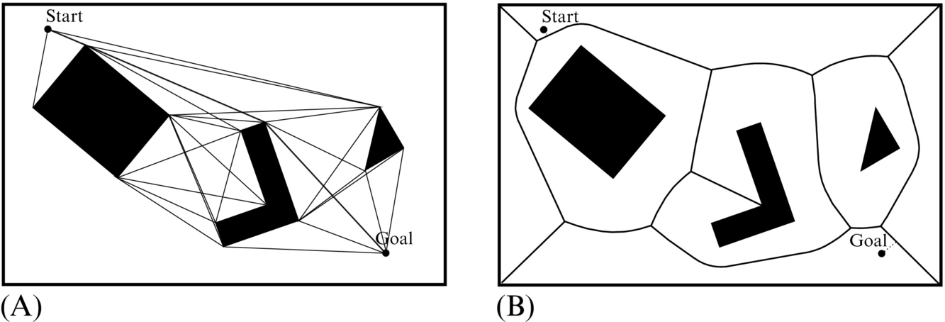
Visibility graphs are simple to use but the number of road connections increases with the number of obstacles, which can result in higher complexity and therefore lower efficiency. A visibility graph can be simplified by removing redundant connections that can be replaced by existing shorter connections.
Voronoi Graph
A Voronoi graph (Fig. 4.11B) consists of road sections that have the largest distance from the obstacles. This also means that the road between any two obstacles has equal distance to both obstacles.
A basic Veronoi graph (diagram) is defined for a plane with n points (e.g., point obstacle). It partitions the plane into n regions whose borders define the roadmap. Each region has exactly one generating point and any point in a certain region is closer to its generating point than to any other generating point. An example of a general Voronoi graph for the plane environment consisting of obstacles of any shape (square, straight line, etc.) is shown in Fig. 4.11. Here, space is partitioned to regions where each region has exactly one generating obstacle. Any point in a certain region is closer to the generating obstacle than to any other obstacle. Borders between the regions define the roadmap.
Driving on such a road minimizes the risk of colliding with obstacles, which can be desired when the robot pose is known with some uncertainty (due to measurement noise or control). In environments constructed from polygons the roadmap consists of three typical Voronoi curves as shown in Fig. 4.12. A Voronoi curve that has equal distance between

• two vertices is a straight line,
• two edges is also a straight line, and
• a vertex and a straight line segment is a parabola.
In a roadmap the start and the goal configuration are also connected, and the obtained graph is used to find the solution.
As already mentioned this approach maximizes robot distance to the obstacles. However, the obtained path length is far from being the optimal (shortest) one. A robot with distance sensors (such as an ultrasonic or laser range finder) can apply a control to drive equally away from all the surrounding obstacles, which means that it follows roads from the Voronoi graph. Although robots using only touch or vicinity sensors cannot follow Voronoi roads because they may have problems with localization, they can easily follow roads in the visibility graph.
Example 4.2
Compute the Voronoi graph for the environment in Fig. 4.11 using the function voronoi in Matlab. The environment (o) and object (o1, o2, o3) coordinates are defined in Listing 4.3.
Solution
In Matlab the Voronoi graph for a list of points can be drawn using a function voronoi. The environment in Fig. 4.11 also contains polygons with defined edges; therefore, the voronoi function cannot be used directly. But if each edge is presented by a number of equidistant (assistant) points, an approximation of the Voronoi graph can be computed (using function voronoi) as shown in Fig. 4.13, where 20 points are used for each obstacle edge.
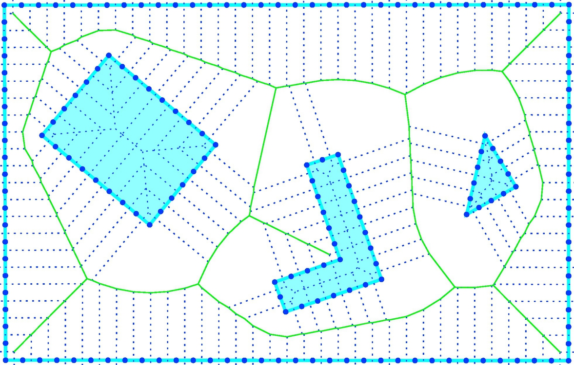
To obtain the final Voronoi graph the obtained cell borders between assistant points belonging to the same edge need to be removed; better yet, they do not need to be computed.
Triangulation
Triangulation is a form of decomposition where the environment is split into triangular cells. Although there are various triangulation algorithms, finding a good triangulation approach that avoids narrow triangles is an open research problem [2]. One possible algorithm is the Delaunay triangulation, which is a dual presentation of the Voronoi graph. In a Delaunay graph the center of each triangle (center of the circumscribed circle) coincides with each vertex of the Voronoi polygon. An example of the latter is given in Fig. 4.14.

From accurate environment decomposition approaches, path searching algorithms can be used in order to determine if the path exists or if it does not. These approaches are therefore complete.
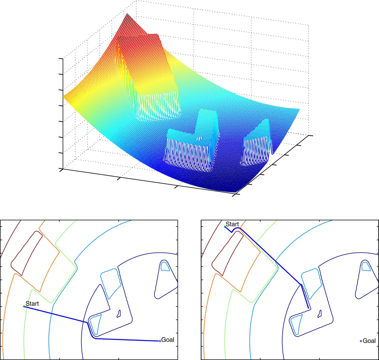
4.2.4 Potential Field
The potential field method describes the environment with the potential field, which can be thought of as an imaginary height. The goal point is in the bottom, and the height increases with the distance to the goal point and is even higher at the obstacles. A path planning procedure can then be explained as the motion of the ball that rolls downhill to the goal, as shown in Fig. 4.15.
A potential field is expressed as a sum of the attractive field due to the goal point Uattr(q) and a repulsive field Urep(q) due to the obstacles:
The goal point is the global minimum of the potential field. Attractive potential Uattr(q) in Eq. (4.1) can be defined to be proportional to the squared Euclidean distance to the goal point ![]() , as follows:
, as follows:

where kattr is a positive constant.
Repulsive potential Urep(q) should be very high near the obstacles and with a decreasing potential as the distance from the obstacles increases D(q, qobst). It should be zero when D(q, qobst) is higher than some threshold value D0. The repulsive potential can be expressed as follows:

where krep is a positive constant and D(q, qobst) is the distance to the nearest point on the nearest obstacle.
To obtain the path from the start to the goal point we need to follow the negative gradient of potential field (−∇U(q)).
Example 4.4
Calculate the negative gradient of the potential field (4.1).
Solution
The negative gradient of attractive field (4.2) equals to

and it is in the direction from the robot pose q to the goal qgoal where the magnitude (norm) is proportional to the distance between the points q and qgoal.
The negative gradient of the repulsive field (4.3) when Dobst ≤ D0 equals
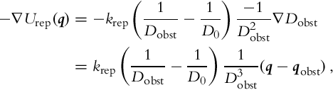
where ![]() . The direction of the repulsive field is always away from the obstacle and its strength decreases with the distance to the obstacle. For situations where Dobst > D0, the repulsive gradient is −∇Urep(q) = 0.
. The direction of the repulsive field is always away from the obstacle and its strength decreases with the distance to the obstacle. For situations where Dobst > D0, the repulsive gradient is −∇Urep(q) = 0.
By using a potential field for environment presentation the robot can reach the goal point simply by following the negative gradient of the potential field. The negative gradient of the potential field is explicitly calculated from the known robot position. The main disadvantage of this approach is the possibility that the robot can become trapped (jittering behavior) in the local minimum, which can happen if the environment contains any obstacle of concave shape (Fig. 4.15) or when the robot starts to oscillate between more equally distanced points to the obstacle. The path planning using a potential field can be used to calculate the reference path that the robot needs to follow, or it can also be used online in motion control to steer the robot in the current negative gradient direction.
4.2.5 Sampling-Based Path-Planning
Up to now the presented path planning methods required explicit presentation of free environment configuration space. By increasing the dimension of the configuration space these methods tend to become time consuming. In such cases, sampling-based methods could be used for environment presentation and path planning.
In sampling-based path planning, random points (robot configurations) are sampled; then collision detection methods are applied in order to verify if these points belong to the free space [4, 5]. From a set of such sampled points and connections among them (connections must also lie in the free space) a path between the known start and the desired goal point is searched.
Sampling-based methods do not require calculation of free configuration space Qfree, which is a time-consuming operation for complex obstacle shapes and for many DOF. Instead, the random samples are used to present the configuration space, and independently from the environment geometry a path planning solution can be obtained for a wide variety of problems. In comparison to decomposition of the environment to cells, the sampling-based approaches do not require a high number of cells and time-consuming computation that is normally required to achieve accurate decomposition to cells. Due to inclusion of stochastic mechanisms (random walk) such as in random path planner the problem of being trapped in some local minimum (e.g., as in the potential field method) is unlikely, because motion is defined between randomly chosen samples from the free space.
To save processing time the collision detection is checked only for obstacles that are close enough and present potential danger of colliding with the robot. Additionally, the robot and obstacles can be encircled by simple shapes so that complex collision detection (between true robot shape and obstacle shapes) is performed only when those enclosing shapes are overlapping. Furthermore, collision detection can be performed hierarchically by exchanging bigger shapes that encircle the whole robot for two smaller shapes that encircle two halves of the robot, as shown in Fig. 4.16. If any of the two shapes are overlapping with the obstacle it is again split in two appropriate smaller shapes. This is continued until the collision is confirmed or rejected or until the desired resolution is reached.

Sampling-based approaches can be divided into the ones that are appropriate for a single path search and those that can be used for many path search queries. In the former approaches the path from a single start to a single goal point needs to be found as quickly as possible; therefore, the algorithms normally focus only on parts of the environment that are more promising to find the solution. New points and connections to the graph are included at runtime until the solution is found. In the latter approaches, the entire procedure of presenting the whole free environment space by an undirected graph or roadmap is performed first. The path planning solution can then be found in the obtained graph for an arbitrary pair of start and goal points. In the following, an example of both approaches is given.
RRT Method
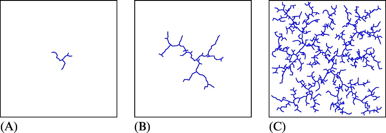
A rapidly exploring random tree (RRT) is the method for searching the path from a certain known start point to one goal point [4]. In each iteration, the method adds a new connection in the direction from the randomly sampled point to the closest point in the existing graph.
In the first iteration of the algorithm the starting configuration qi presents the graph tree. In each next iteration a configuration qrand is chosen randomly and the closest node qnear from the existing graph is searched for. In the direction from qnear to qrand at some predefined distance ε a candidate for a new node qnew is calculated. If qnew and the connection from qnear to qnew are in the free space then qnew is selected as the new node and its connection to qnear is added to the graph. The procedure is illustrated in Fig. 4.17.

The search is complete after some number of iterations are evaluated (e.g., 100 iterations) or when some probability is reached (e.g., 10%). Once the algorithm termination criterion is satisfied, the goal point is selected instead of taking a new random sample, and a check is made to determine whether the goal point can be connected to the graph [6]. Such a graph tree is quickly extending to unexplored areas as shown in Fig. 4.18. This method has only two parameters: the size of the step ε and the desired resolution or number of iterations that define the algorithm termination conditions. Therefore, the behavior of the RRT algorithm is consistent and its analysis is simple.
PRM Method
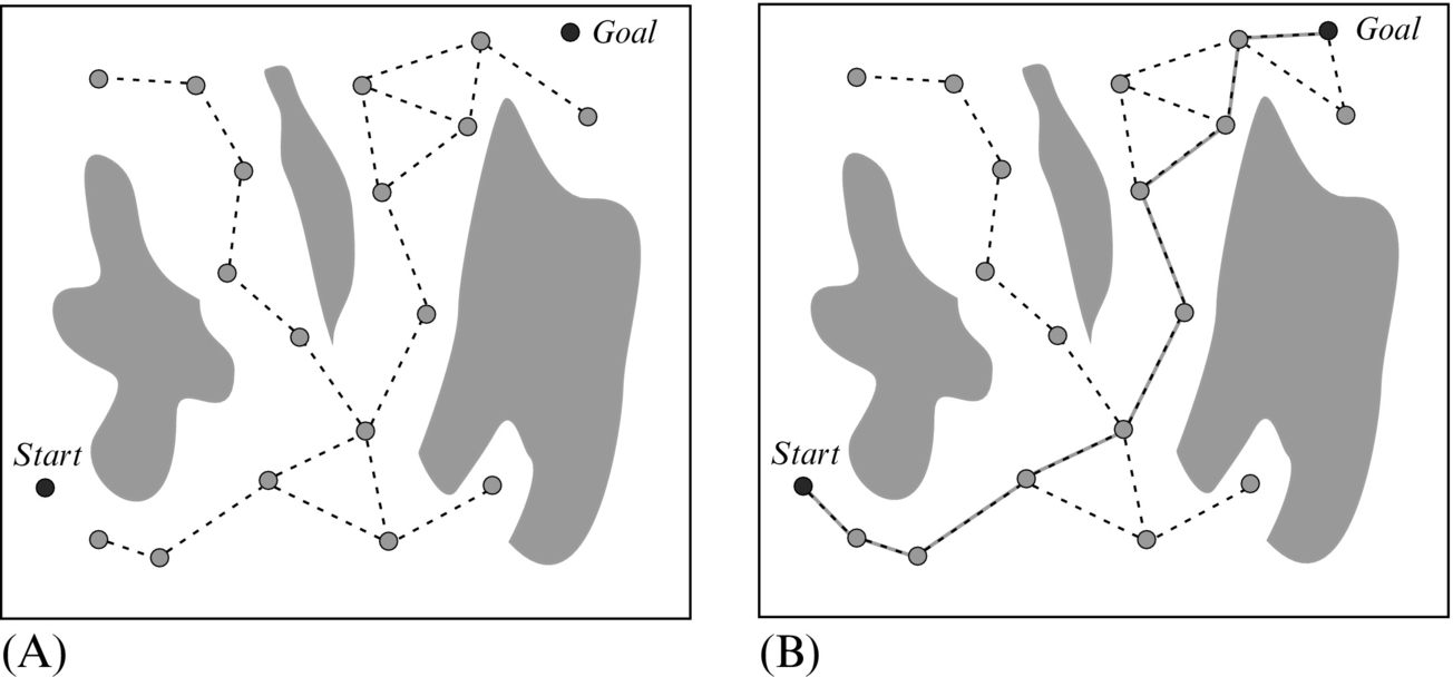
A probabilistic roadmap (PRM) is the method used for path searching between more start points and more goal points [7]. The algorithm has two steps. The first step is the learning phase where a roadmap or undirected graph of the free space is constructed as shown in Fig. 4.19A. In the second step the current start and goal point are connected to the graph and some graph path searching algorithm is used to find the optimum path, as shown in Fig. 4.19B.
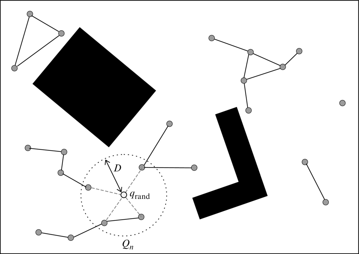
In the learning phase a roadmap is constructed. The roadmap is initially an empty set and it is later filled with nodes by repeating the following steps. A randomly chosen configuration qrand from the free space is included in the map, and nodes Qn that are needed to expand the map are found. These nodes can be found by choosing K nearest neighbor nodes (Qn) or all neighbor nodes whose distance to qrand is smaller than some predefined parameter D, as shown in Fig. 4.20. Note that in the first iteration or at first few iterations neighbor nodes probably cannot be found. All simple connections from qrand to the nodes Qn that entirely lie in the free space are included in the map. This procedure is repeated until the map contains the desired number of N nodes.
In the path searching phase the desired start and the goal point are connected through free space with the closest possible nodes from the map. Then a path searching algorithm is applied to find the path from the start to the goal point.
These two phases do not need to be performed separately, as they can be repeated iteratively until the current number of nodes is high enough to find the solution. If the solution cannot be found, the map is further expanded with new nodes and connections until the solution is feasible. In this way we iteratively approach toward the most appropriate presentation of the free space.
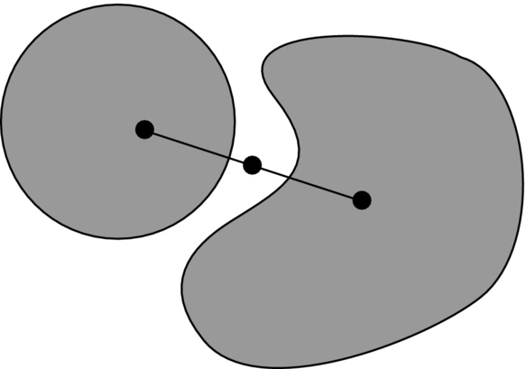
This method is very effective for robots with many DOF; however, there can be problems finding the path between two regions that are connected with a narrow passage. This problem can be solved by adding additional nodes using the bridge test, where three nearby random points on some straight line is selected, as shown in Fig. 4.21. If the outermost points are in collision with the obstacle and the middle one is not, then the latter is included as a node in the map. We try to connect this node with neighbor nodes in a similar way as other connections and add these connections to the map. By combining a bridge test with uniform sampling into some hybrid sampling strategy [8], smaller roadmaps that cover free space efficiently and still have good connectively in narrow passages can be obtained.
4.3 Simple Path Planning Algorithms: Bug Algorithms
Bug algorithms are the simplest path planning algorithms that assume only local knowledge and do not need a map of the environment. Therefore, they are appropriate in situations where an environment map is unknown or it is changing rapidly and also when the mobile platform has very limited computational power. These algorithms use local information obtained from their sensors (e.g., distance sensor) and global goal information. Their operation consists of two simple behaviors: motion in a straight line toward the goal and obstacle boundary following.
Mobile robots that use these algorithms can avoid obstacles and move toward the goal. These algorithms require low memory usage and the obtained path is usually far from being optimal. Bug algorithms were first implemented in [9] and several improvements followed such as in [10–12].
In the following three basic versions bug algorithms are described.
4.3.1 Bug0 Algorithm
A Bug0 algorithm has two basic behaviors:
1. Move toward the goal until an obstacle is detected or the goal is reached.
2. If an obstacle is detected, then turn left (or right, but always in the same direction) and follow the contour of the obstacle until motion in a straight line toward the goal is again possible.
A example of Bug0 algorithm performance is given in Fig. 4.22.
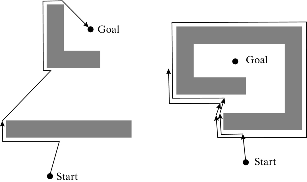
4.3.2 Bug1 Algorithm
A Bug1 algorithm in comparison to Bug0 uses more memory and requires several more computations. In each iteration it needs to calculate Euclidean distance to the goal and remember the closest point on the obstacle circumference to the goal. Its operation is described by the following:
1. Move on the straight line toward the goal until an obstacle is hit or the goal is reached.
2. If an obstacle is detected, then turn left and follow the entire contour of the obstacle and measure the Euclidean distance to the goal. When the point where the obstacle was initially detected is reached again, follow the contour of the obstacle in the direction that is shortest to the point on the contour that is closest to the goal. Then resume moving toward the goal in a straight line.
A example of a Bug1 algorithm operation is given in Fig. 4.23.
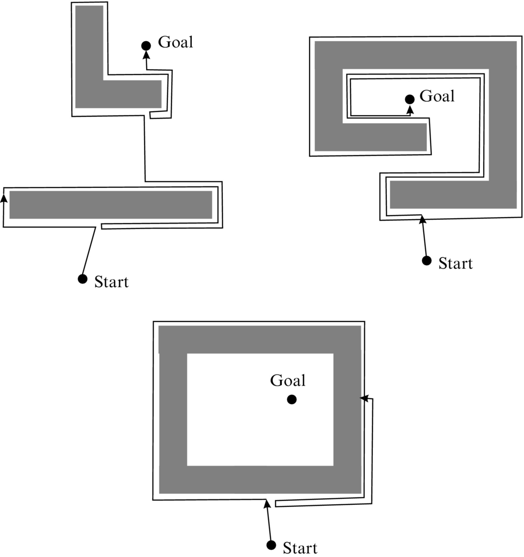
 of the length of all obstacle contours longer than the Euclidean distance from the start to the goal configuration. The algorithm can identify unreachable goal.
The obtained path is not optimal and is in the worst case for ![]() of the length of all obstacle contours longer than the Euclidean distance from the start to the goal configuration. For each obstacle that is detected on its path from the start to the goal, the algorithm finds only one entry point and one leaving point from the obstacle contour. So it never detects the obstacle more than once and therefore never circles among the same obstacles. When the algorithm detects the same obstacle more than once it knows that either the start or the goal point is captured inside the obstacle and the path searching can be terminated, since no feasible path to the goal exists (bottom situation in Fig. 4.23).
of the length of all obstacle contours longer than the Euclidean distance from the start to the goal configuration. For each obstacle that is detected on its path from the start to the goal, the algorithm finds only one entry point and one leaving point from the obstacle contour. So it never detects the obstacle more than once and therefore never circles among the same obstacles. When the algorithm detects the same obstacle more than once it knows that either the start or the goal point is captured inside the obstacle and the path searching can be terminated, since no feasible path to the goal exists (bottom situation in Fig. 4.23).
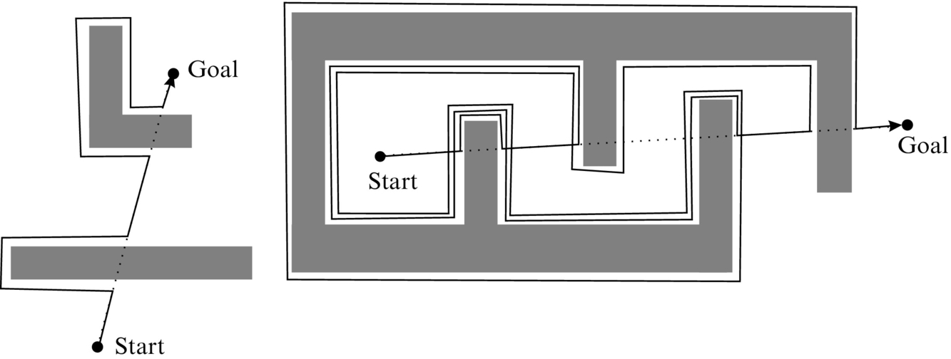
4.3.3 Bug2 Algorithm
The Bug2 algorithm always tries to move on the main line that is defined as a straight line connecting the start point and the goal point. It operates by repeating the following steps:
1. Move on the main line until an obstacle is hit or the goal point is reached. In the latter case the path searching is finished.
2. If an obstacle is detected, follow the obstacle contour until the main line is reached where the Euclidean distance to the goal point is shorter than the Euclidean distance from the point where the obstacle was first detected.
Although the Bug2 algorithm in general seems much more effective than Bug1 (see left part of Fig. 4.24), it does not guarantee that the robot detects certain obstacles only once. At some obstacle configurations the robot with Bug2 could make unnecessary repeating obstacle encirclements until it reaches the goal point as illustrated in the right part of Fig. 4.24. The algorithm can identify that the goal is unreachable if it comes across (detects) the same obstacle in the same point more than once.
From comparison of Bug1 and Bug2 algorithms the following can be concluded:
• Bug1 is the more thorough search algorithm, because it evaluates all the possibilities before making a decision.
• Bug2 is the greedy algorithm, because it selects the first option that looks promising.
• In most cases the Bug2 algorithm is more efficient than Bug1.
• However, the operation of the Bug1 algorithm is easier to predict.
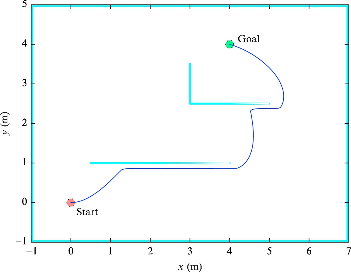
Example 4.9
Implement path planning using Bug0 algorithm for a mobile robot with differential drive. Assume that the environment map is not available and the robot only knows its current pose, goal point, and current distance to the goal (measurement from sensor).
According to the Bug0 algorithm the robot should drive toward the goal if it is far enough from any obstacle (e.g., more than 0.2 m), and it should follow the obstacle if it is close to the obstacle. Code your implementation of the algorithm in the simulation framework given in Listing 4.8, which already enables simulation of robot motion and sensor measurements. The environment and an example of an obtained robot path are shown in Fig. 4.25.
4.4 Graph-Based Path Planning Methods
If the environment with obstacles is sufficiently presented by a graph, one can use path searching algorithms to find the path from the start to goal configuration. In the following, a few well-known path graph-based searching algorithms are presented.
In general, path searching algorithms proceed as follows. The starting node is first checked to determine if it is also the goal node. Normally this is not the case; therefore, the search is extended to other nodes in the neighborhood of the current node. One of the neighbor nodes is selected (how the nodes are selected depends on the used algorithm and its cost function), and if it is not the goal node, then the search is also extended to the neighbor nodes of this new node. This procedure is continued until the solution is found or until all graph nodes have been investigated.
When performing a search in a graph, a list of nodes that have already been visited is made with the main purpose to prevent visiting the same node more than once. Nodes that can still extend the search area to other neighbor nodes (also known as alive nodes) are kept in an open list. Nodes that have no successors or have been checked already (also known as dead nodes) are kept in a closed list.
The evolution of path searching depends on the strategy of selecting new nodes for extending the search area. A list of open nodes is sorted according to some criteria and when the search is extended the first node from that sorted list is taken; this node best fits the used sorting criteria (has the smallest value of the criteria).
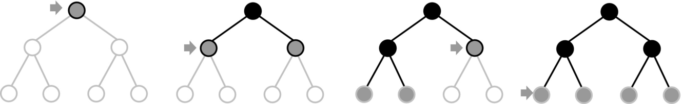
In the beginning, the open list Q only contains the start node. Nodes in the neighborhood of the start node are calculated and put in the open list, and the starting node is put in the closed list. The search is then extended with the first node in the open list and successors (of the chosen node from the open list) are calculated. The open list then contains the remaining previous successors (except the first one that has been already extended) and currently calculated successors of the chosen node. This procedure is shown in Fig. 4.26, where nodes in the open list are colored with light gray, nodes in the closed list are colored black and unvisited nodes are white. In Fig. 4.26 it can be seen why the nodes from the open list are called leaf nodes.
Graph search algorithms can be classified as informed or noninformed. Noninformed algorithms use no additional information beside the problem definition. These approaches search the graph systematically and do not distinguish more promising nodes from the less promising ones. Informed search, also known as heuristic search, contains additional information about the nodes. Therefore, it is possible to select more promising nodes and in that way searching for the final solution can be more efficient.
4.4.1 Breadth-First Search
Breadth-first search belongs to a class of noninformed graph search algorithms. It first explores the shallow nodes, that is, the nodes that are closest to the starting node. All nodes that can be accessed in k steps are visited before any of the nodes that require k + 1 steps (Fig. 4.26).
In the open list Q, the nodes are sorted using a FIFO approach (first-in first-out). The newly opened nodes are added to the end of the list Q and the nodes for extending the search are taken from the beginning of the list Q.
The algorithm is complete because it finds solution if it exists. If there exist several solutions, it finds the one that has the least steps from the starting node. In general, the found solution is not optimal because it is not necessary that all transitions between nodes have equal cost.
The algorithm generally requires high memory usage and long computing times. Computational time and memory consumption both increase exponentially as graph branching progresses.
4.4.2 Depth-First Search
Depth-first search is a noninformed graph search algorithm where the search is first extended in the depth. The node that is the farthest away from the starting node is used to extend the search. The search continues in the depth until the current node has no further successors. The search is then continued with the next deepest node whose successors have not been explored yet, as shown in Fig. 4.27.

The list of open nodes Q is a stack sorted by the LIFO (last-in first-out) method. The newly opened nodes are added to the beginning of the list Q and from the same end; also, the nodes for extending the search area are taken.
The depth-first search is not complete. In the case of an infinite graph (with infinite branch that does not end), it can get trapped in one branch of the graph; or in the case of a loop branch (loop in finite graph depth), it can get stuck in cycles. To avoid this problem the search can be limited to a certain depth only, but then the solution can have a higher depth than the maximum depth limitation. The algorithm is also not optimal because the found path is not necessarily the shortest one also.
This method has low memory usage as it only stores the path from the start node to the current node and intermediate nodes that have not been explored yet. When some nodes and all of their successors are explored, this node no longer needs to be stored in the memory.
4.4.3 Iterative Deepening Depth-First Search
This algorithm combines advantages of the breadth-first search and depth-first search algorithms. It iteratively increases the search depth limit and explores nodes using the depth-first search algorithm until the solution is found (Fig. 4.28). First, the depth-first search is performed for the nodes that are zero steps away from the starting node. If the solution is not found, the search in the depth is repeated for nodes that are up to one step away from the starting one and so on.
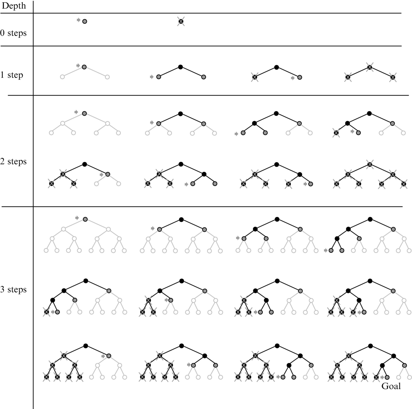
This algorithm is complete (the solution is found if it exists), and it has small memory usage and is optimal if the cost of all transitions are equal or if transition costs increase with the node depth. If all the nodes have approximately the same rate of branching, then the repeated calculation of nodes is also not a big computational burden because the majority of the nodes are in the bottom of the tree, and those nodes are visited only once or a few times.
4.4.4 Dijkstra’s Algorithm
Dijkstra’s algorithm is a noninformed algorithm that finds the shortest paths from one node (source node) to all the other nodes in the graph [13]. The result is therefore the shortest path tree from the source node to any other node. Originally it was proposed by Dijkstra [14] and later extended with many modifications. In problems where the shortest path between one starting node and one goal node must be found Dijkstra’s algorithm may seem inefficient due to calculation of optimum paths to all the other nodes. In this case the algorithm can be terminated as soon the shortest desired path is calculated.
The algorithm finds the shortest path between the starting (source) node and the goal node because it calculates the cost function for the path between the start node to the current node, which we name cost-to-here. The cost of the path to the current node (cost-to-here) is calculated as the sum of the path cost to the previous node (from which we came to the current node) and the cost of the transition between the previous node and the current node. In the case of several shortest paths (paths with the same cost) the algorithm returns only one, and it is not important which one.
To run the algorithm the transitions between the nodes and their costs need to be defined. For each visited node the algorithm stores the cost of currently shortest path to it (cost-to-here) and the connection from where we arrived to the current node. During the search, the lists of open nodes and closed nodes are adapted.
The operation of the algorithm is as follows. At the beginning, the open list contains only the start node, which has zero cost-to-here and it is without a connection to a previous node. The list of closed nodes is empty. Then the following steps (also shown in Fig. 4.29) are performed.

 .
.1. From the open list take the first node; call it the current node. The open list is sorted according to the cost-to-here in increasing order, where the first node is the one with the smallest cost-to-here.
2. For all nodes that can be reached from the current node calculate the cost-to-here as a sum of the current node’s cost-to-here and transition cost.
3. Calculate and store cost-to-here and appropriate connection to the current node for all the nodes that do not already have these information stored.
4. If in the previous step some nodes already have cost-to-here and appropriate connection from some previous iteration, then compare both costs-to-here and keep in storage the lower cost-to-here and its connection.
5. Nodes are added to the open list and sorted in increasing order of the costs-to-here. Such a list is called a priority queue and enables that the node with the lowest price-to-here is found faster than in an unsorted list. The current node is moved to the closed list.
Originally, Dijkstra’s algorithm terminates when the open nodes list is empty and the result are the shortest paths from the starting node to all the other nodes. If only the shortest path from the starting node and some goal node is needed then the algorithm terminates when the goal node is added to the closed list.
The resulting path can be obtained by back-tracking the connections that brought us to the goal node. At the goal node the connection to the previous node is obtained then the connection to its previous node is read and so on until the start node is reached. Finally, the obtained list of connections is inverted.
Dijkstra’s algorithm is complete and optimal algorithm if all the connections have costs higher than zero.
4.4.5 A* Algorithm
A* (A star) is an informed algorithm because it includes additional information or heuristic. Heuristic is the cost estimate of the path from the current node to the goal that is for the part of the graph tree that has not been explored yet. This enables the algorithm to distinguish between more or less promising nodes, and consequentially it can find the solution more efficiently. For each node the algorithm computes the heuristic function that is the cost estimate for the path from this node to the goal, and it is called cost-to-goal. This heuristic function can be Euclidean distance or Manhattan distance (sum of vertical and horizontal moves) from the current node to the goal node. The heuristic can be computed also by some other appropriate function.
During algorithm execution for each node the cost of the whole path (cost-of-the-whole-path) is calculated to consist of cost-to-here and cost-to-goal. During the path search, the open nodes list and closed nodes list are also used.
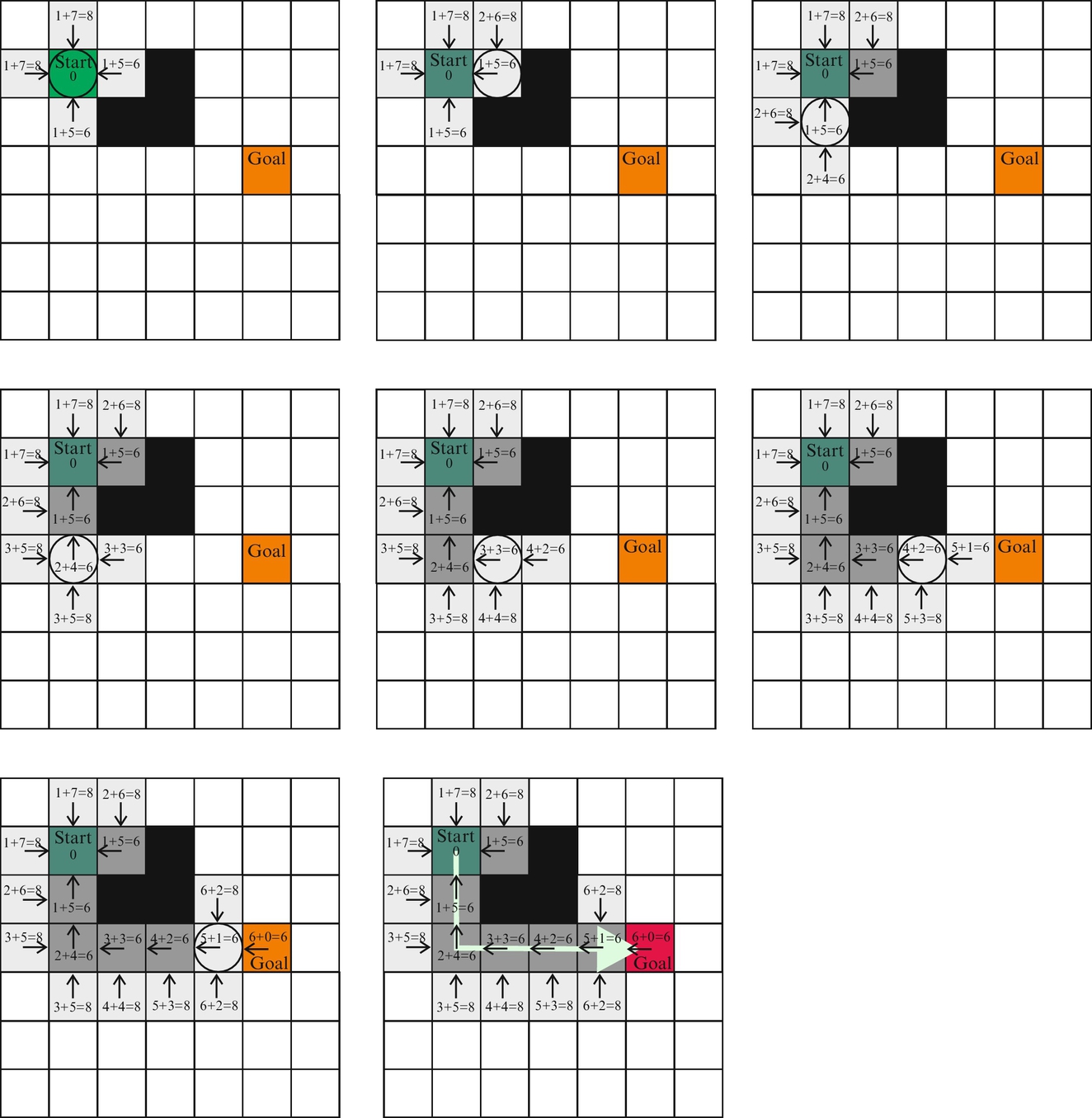
The algorithm operation is as follows. In the beginning, the open list contains only the starting node, which has zero cost-to-here and is without a connection to a previous node. Then the following steps (also illustrated in Fig. 4.30) are repeated.
1. From the open list the first node is taken; it is called the current node. The open list is sorted according to the cost-of-the-whole-path in increasing order, where the first node is the one with the smallest cost-of-the-whole-path.
2. For all nodes that can be reached from the current node we calculate the following:
• cost-to-here as the sum of the cost-to-here of the current node and the transition cost, and
• cost-of-the-whole-path as the sum of cost-to-here and cost-to-goal.
3. For each of those nodes that do not already have stored cost-to-here, the values of the connection from the current node, cost-to-goal, and cost-of-the-whole-path are stored.
4. If in the previous step some node already has stored the cost values from some previous iteration, then both costs-to-here (current and the previous one) are compared and the one with a lower value is stored, alongside with the corresponding connection and cost-of-the-whole-path.
5. Nodes whose cost values have been calculated for the first time are added to the open list. The nodes that have already been in the open-list and were updated are kept in the open list. The nodes that have been updated and were in the closed list are moved to the open-list. The open list is sorted according to the cost-of-the-whole-path in increasing order. The current node is transferred to the closed list.
In the first subfigure (in Fig. 4.30) the current node is the start node and its successor nodes (accessed in four directions: left, right, up, and down from the current node) are selected. For all the successor nodes, the cost-to-here is one as they are only one step away from the star node and cost-to-goal is the Manhattan distance (heuristic) from the successor node to the goal node, which can also be measured through the obstacle. The sum of both costs is the cost-of-the-whole path. The successors nodes also have a connection marked by an arrow (direction) to its parent node (current node marked by a circle). The open list now contains these four successor nodes and closed list contains the starting node.
In the second subfigure (in Fig. 4.30) the node with the lowest cost-of-the-whole path (with cost 6) is selected from the open list as the current node. The current node has only one successor (other cells are blocked by the obstacle or in the closed list). Cost-to-here for this successor node is 2 as it is two steps away (Manhattan distance) from the start node and cost-to-goal is 8. The current node is put to the closed list and the successor node to the open list. In the third subfigure (in Fig. 4.30) the current node becomes the node from the open list with the lowest cost-of-the-whole path, which is 6. Then the algorithm continues similarly as in the first two steps.
The A* algorithm is guaranteed to find the optimal path in graph if the heuristic for calculation of the cost-to-goal is admissible (or optimistic), which means that the estimated cost-to-goal is smaller or equal to true cost-to-goal. The algorithm finishes when the goal node is added to the closed list.
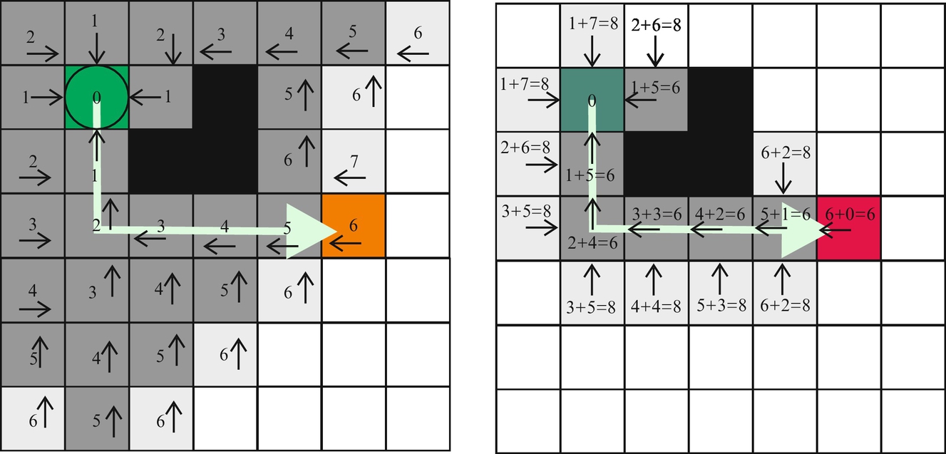
The A* algorithm is a complete algorithm because it finds the path if it exists, and as already mentioned, it is optimal if the heuristic is admissible (optimistic). Its drawback is large memory usage. If all costs-to-goal are set to zero the A* operation equals Dijkstra’s algorithm. In Fig. 4.31 a comparison of Dijkstra’s and A* algorithm performance is shown.
4.4.6 Greedy Best-First Search
Greedy best-first search is the informed algorithm. The open list is sorted in the increasing cost-to-goal. Therefore, the search in each iteration is extended to the open node that is closest to the goal (has the smallest cost-to-goal) assuming it will reach the goal quickly. The found path is not guaranteed to be optimal as shown in Fig. 4.32. The algorithm only considers cost from the current node to the goal and ignores the cost required to come to the current node; therefore, the overall path may become longer than the optimum one. Because the algorithm is not optimal it is also not necessary that the heuristic is admissible as it is important in A*.
