
Image Features
Several nice properties of the camera, computational capabilities of modern computers, and advances in the development of algorithms make the use of a camera an extremely appealing sensor for solving problems in robotics. A camera can be used to detect, identify, and track observed objects in the camera’s field of view, since images are projections of the 3D objects in the environment (see Section 5.2.4). The digital image is a 2D discrete signal that is represented with a matrix of quantized numbers that represent either the presence or absence of light, light intensity, color, or some other quantity. The main types of images are color (Fig. 5.22A), grayscale (Fig. 5.22B), and binary (Fig. 5.22C). In machine vision grayscale images are normally sufficient when looking for particular patterns that are not color dependent. Binary images are seldom a result of image segmentation or are used for content masking. One of the simplest image segmentation methods is thresholding, where pixels with a grayscale level above a threshold are marked with a logical one, and all the other are set to logical zero. For example, thresholding grayscale image in Fig. 5.22B with a threshold of 70 results in a binary in Fig. 5.22C. The frequency of grayscale levels can be presented in a histogram that can be used in order to determine the most appropriate threshold level. In Fig. 5.22D a histogram with 256 bins that corresponds to 256 levels of the grayscale image in Fig. 5.22B is shown.

Over the recent years many machine vision algorithms have been developed that enable image-based object tracking. For this purpose image content is normally represented with image features. Features can be image regions with similar properties (e.g., similar color), patches of a particular pattern, or some other image cues (e.g., edges, corners, lines). In some situations artificial markers can be introduced into the environment that enable fast and reliable feature tracking (e.g., color markers or matrix barcodes to track mobile soccer robots). When this is not possible features need to be extracted from the image of a noncustomized scene. In some applications simple color segmentation can be used (e.g., detection of red apples in an orchard). In the recent years many approaches have been developed that enable extraction of natural local image features that are invariant to some image transformations and distortions.
Color Features
Detection of image regions with similar colors is not a trivial task due to inhomogeneous illumination, shadows, and reflections. Color-based feature tracking is therefore normally employed only in the environments where controlled illumination conditions can be established or the color of the tracked object is distinctive enough from all the other objects in the environment.
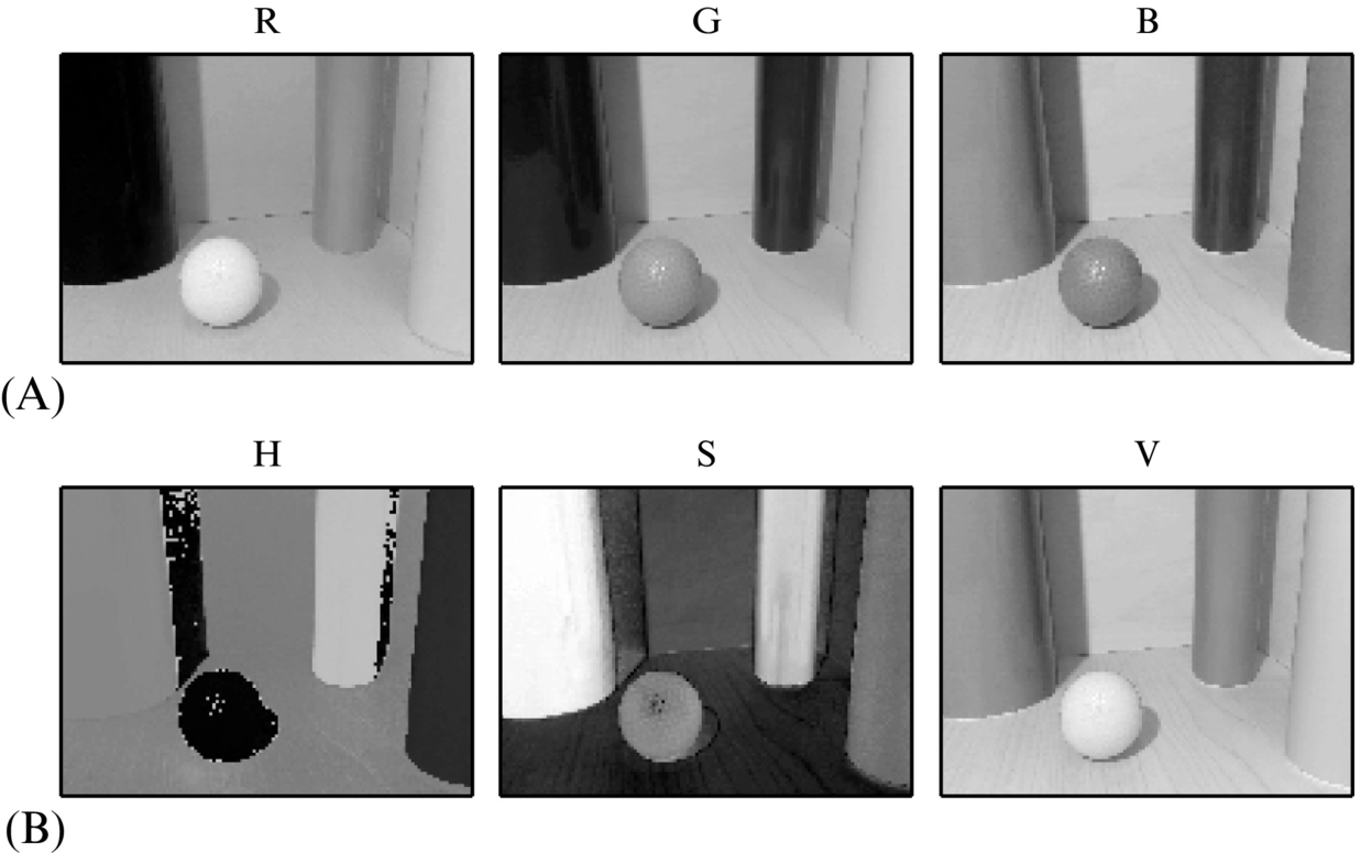
Color in a digital image is normally represented with three color components: red, green, and blue; this is known as the RGB color model. The color is restored from a combination of red, green, and blue color components that are filtered through red, green, and blue color filters, respectively. Two other color spaces that are seldom used in machine vision are HSL (hue-saturation-lightness) and HSV (hue-saturation-value). HSV color space is seldom used since it enables a more natural description of colors and better color segmentation than can be achieved in RGB space. The values from the RGB color space given in the range [0, 255] can be converted to HSV color space according to the following:

where ![]() and
and ![]() . In Eq. (5.87) the saturation S and value V are in the range [0, 1], and the hue H is in the range [0, 360) that corresponds to angular degrees and wraps around. In Fig. 5.23 RGB and HSV components of the color image in Fig. 5.22A are shown.
. In Eq. (5.87) the saturation S and value V are in the range [0, 1], and the hue H is in the range [0, 360) that corresponds to angular degrees and wraps around. In Fig. 5.23 RGB and HSV components of the color image in Fig. 5.22A are shown.
Color histograms can be used to segment regions of a particular color. HSV histograms (with 32 bins) of several templates with similar color are shown in Fig. 5.24 (the color regions have been extracted from the image in Fig. 5.22A). Histograms of each template can be back-projected to the original image, that is, for every pixel in the image the frequency of the bin that belongs to the value of the pixel in the corresponding color channel in the image is set. The resulting back-projected grayscale images can be merged together as a linear combination of color channels. The results of blue, orange, red yellow, and wood color HSV histogram back-projection is shown in the first column of Fig. 5.25. In the resulting image the grayscale levels represent the measure of similarity of the pixels to the color template. Before the image is thresholded (see the third column in Fig. 5.25) some additional image filtering can be applied. The image can be smoothed with a 2D Gaussian filter (see the second column in Fig. 5.25) to remove some noisy peaks. The thresholded binary image can be filtered with, for example, some morphological or other binary image processing operations to remove or fill some connected regions. The resulting image mask (see the fourth column in Fig. 5.25) can be used to filter out the detected regions in the original image (see the last column in Fig. 5.25). More on image processing algorithms can be found, among others, in [10]. In practical implementations of color-based image segmentation some filtering processes are skipped in order to speed-up algorithms’ performance for the price of accuracy. Sometimes every pixel in the input image is considered part of the object if the color values of all components are within some lower and upper bounds that correspond to some color. In Fig. 5.24 it can be observed that hue and saturation values enable simple segmentation of colors. However, it should be pointed out that color-based segmentation is sensitive to changing illumination conditions in the environment. Although some approaches can compensate for inhomogeneous illumination conditions [11], the color-based image segmentation is the most commonly used only in situations where appropriate illumination conditions can be achieved.


The results of image segmentation is a binary image where image pixels that belong to the object are set to a nonzero value and all the other points are set to zero. There may be several or only a single connected region. If there are several connected regions an appropriate algorithm needs to be applied in order to find the positions and shapes of these objects [11]. To make searching of connected regions more robust some constraints can be introduced that reject areas with too small or too big areas, or some other region property. If the observed object is significantly different from the surrounding environment in a way that it can be robustly detected as a single region in a segmented image, the position and shape of this image region can be described with image moments.
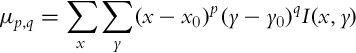
The definition of a raw moment of a (binary) digital image I(x, y) is the following:

where p and q are positive integers (p + q is the order of the moment). The moment m0, 0 represents object mass that is equal to the area of the object in the case of a binary image. Zero- and first-order raw moments can be used in order to find the center of the object (x0, y0) in the binary image:

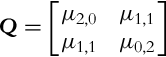
To describe object orientation and shape central moments can be used:
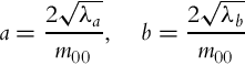
which are invariant to in-image translation. Central moments can be used to fit an ellipsoid to the detected object in the image. The ellipse’s semimajor axis a and semiminor axis b can be obtained from eigenvalues λa and λb (λa ≥ λb) of the matrix Q, which consists of second-order central moments:
The ellipse axes are
The orientation of the semimajor ellipse axis is given by the angle θ:
In Fig. 5.26 raw and central moments have been used in order to fit an ellipsoid over the binary patch (the result of orange color segmentation from Fig. 5.25). The way ellipsoid parameters can be obtained from image moments is shown in Listing 5.14, where central moments were derived from raw moments. As it can be seen, image moments can be used to describe simple image features and determine locations of the features in an image. In [12] another set of moments is defined that are invariant to scale, translation, and rotation.

Artificial Pattern Markers
The introduction of artificial markers presents a minimal customization of the environment that can significantly simplify some vision-based tasks like, for example, object tracking, camera pose estimation, etc. An artificial pattern marker is a very distinctive pattern that can be robustly detected. A sample set of three artificial markers is shown in Fig. 5.27. Marker patterns are normally designed in a way that the markers can be reliably and precisely detected. Moreover, in the pattern of the marker, the marker ID is encoded; therefore, multiple markers can be tracked and identified through a sequence of images. One of the popular artificial marker detection algorithms is ArUco [13, 14]. Fig. 5.28 shows the detected artificial markers from Fig. 5.27 in two camera views.


The algorithms for detection of artificial markers normally consist of a marker localization step, in which the position, orientation, and size of the marker is determined. This procedure needs to robustly filter out only true markers from the rest of the objects in the environment. Once the locations of markers in the image are known, the projection between the detected marker and marker’s local coordinate frame can be established. Based on the pattern of the marker in the transformed local marker coordinate frame the ID of the marker is determined. Some artificial marker patterns are designed in a way that enable pattern correction that makes identification of patterns more reliable and also robust to noise and occlusions.
Natural Local Image Features
Images contain features that are inherently present in the environment. Over the years many machine vision algorithms have been developed that enable automatic detection of local features in images. Some of the important local feature algorithms are SIFT (Scale Invariant Feature Transform) [15], SURF (Speeded-Up Robust Features) [16], MSER (Maximally Stable Extremal Regions) [17], FAST (Features from Accelerated Segment Test) [18], and AGAST (Adaptive and Generic Accelerated Segment Test) [19]. Most of these algorithms are included in the open source computer vision library OpenCV [20, 21]. In robotic applications an important property of description of images with features is the algorithm efficiency to enable real-time performance. Different approaches have been developed for local feature extraction (localization of features), local feature description (representation of feature properties), and feature matching.
The goal of feature extraction is to detect and localize points of interest (local regions), normally in order to reduce the dimensionality of the raw image. Most commonly the features are extracted from grayscale images. Feature extractors can detect different types of image patterns: edges (e.g., Canny filter, Sobel filter, and Roberts cross), corners (e.g., Harris and Hessian operator, FAST), blobs (e.g., Laplacian of Gaussian, difference of Gaussians, MSER). To enable detection of features of different sizes, the raw image is seldom represented in scale-space [15]. Feature extraction should be invariant to some class of image transformations and distortions to enable repeatable detection of features across multiple views of the same scene. Normally it is desired that features are invariant to image translation, rotation, scaling, blur, illumination, and noise. Features should also be robust to some partial occlusions. The desirable property of the features is therefore locality. In mobile robotic applications it is normally required that features are also detected accurately and that the quantity of the features is sufficiently large, since this is a common prerequisite for accurate and robust implementation of algorithms that depend of extracted features (e.g., feature-based mobile robot pose estimation). An example of detected features in two camera views of the same scene is shown in Fig. 5.29. Every feature is given with position, orientation, and size.
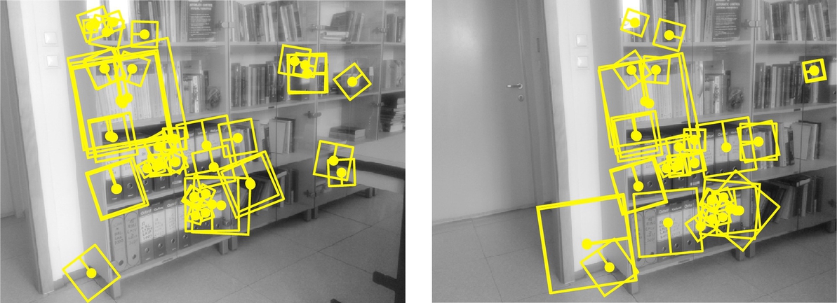
The purpose of feature description is to describe each feature (based on the properties of the image pattern around the feature) in a way that enables identification of the same features across multiple images if the features reappear in the other images. The local pattern around the feature (e.g., the region marked with a square in Fig. 5.29) is used in order to determine the appropriate feature descriptor, which is normally represented as a feature vector. Local feature descriptors should be distinctive in a way that accurate feature identification is enabled regardless of different variations in the environment (e.g., illuminations changes, occlusions). Although local image features could be directly compared with, for example, convolution of local feature regions, this kind of approach does not have appropriate distinctiveness, and it is also quite computationally demanding. Feature descriptor vectors tend to be a minimal representation of features that enable an adequate level of feature distinctiveness for reliable feature matching. Which feature extractor and feature is used depends on the particular application. An experimental comparison of various feature detectors can be found in, for example, [22]. An example of two sets of feature description vectors of features extracted from the left and right image in Fig. 5.29 is graphically represented in Fig. 5.30.

Feature matching is one of the basic problems in machine vision. Many machine vision algorithms—like scene depth estimation, image-based 3D scene reconstruction, and camera pose estimation depend on appropriate feature matches between multiple images. Features can be matched by comparing the distances between the feature descriptors (vectors). Depending on the type of feature descriptor different distance measures can be used. Normally Euclidean or Manhattan distance is used for real-valued feature descriptors, and Hamming distance is used for binary feature descriptors. Due to imprecise feature localization, feature distortions, and repeated patterns, feature description matching does not always provide appropriate matches. Therefore an appropriate feature matching technique should be used that can eliminate spurious matches.
Given two sets of feature descriptors ![]() and
and ![]() , the matching process should find the appropriate feature matches between the two sets. For every feature in the set
, the matching process should find the appropriate feature matches between the two sets. For every feature in the set ![]() the closest feature in the set
the closest feature in the set ![]() (according to selected feature distance measure) can be selected as a possible match candidate. This is in general a surjective mapping, since some features in set
(according to selected feature distance measure) can be selected as a possible match candidate. This is in general a surjective mapping, since some features in set ![]() can have more than only one match from set
can have more than only one match from set ![]() . In normal conditions a feature in one set should have at most a single match in the other set. To overcome this issue, normally a two-way search is performed (i.e., for every feature in set
. In normal conditions a feature in one set should have at most a single match in the other set. To overcome this issue, normally a two-way search is performed (i.e., for every feature in set ![]() the closest feature in set
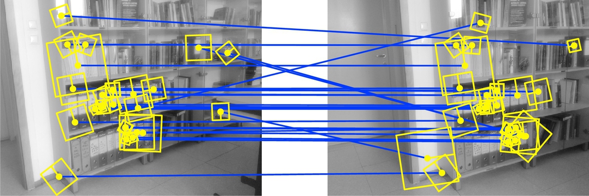
the closest feature in set ![]() is found and vice versa) and only matches that are the same in both searches are retained. Additionally, if the distance between the best and the second best match is too small (below a selected threshold), the matched pair of features should be rejected, since there is a high probability of matching error. Also the pair of features should be rejected, if the distance between the matched feature descriptors is above a certain threshold, since this implies too high feature dissimilarity. In Fig. 5.30 the matches between two sets of feature descriptors are shown. Although the aforementioned filtering techniques were applied, not all incorrect matches were removed, as it is seen in Figs. 5.31 and 5.32 that there are still some incorrect matches. It should be noted that even if there are only a few outliers, these can have a significant influence on the results of the estimation algorithms that assume the features are matched correctly.
is found and vice versa) and only matches that are the same in both searches are retained. Additionally, if the distance between the best and the second best match is too small (below a selected threshold), the matched pair of features should be rejected, since there is a high probability of matching error. Also the pair of features should be rejected, if the distance between the matched feature descriptors is above a certain threshold, since this implies too high feature dissimilarity. In Fig. 5.30 the matches between two sets of feature descriptors are shown. Although the aforementioned filtering techniques were applied, not all incorrect matches were removed, as it is seen in Figs. 5.31 and 5.32 that there are still some incorrect matches. It should be noted that even if there are only a few outliers, these can have a significant influence on the results of the estimation algorithms that assume the features are matched correctly.

Some matched features may not satisfy system constraints: for example, if two matched features do not satisfy the epipolar constraint or if the reconstructed 3D point from the matched features would appear behind the camera, the match should be rejected. More constraints can be found in [23]. In wheeled mobile robotics additional constraints can be introduced based on the predicted robot states from known actions and the kinematic model. Incorporating a model of some geometric constraints into the feature matching process can be used to filter out the matched feature pairs that are not physically possible. For this purpose some robust model-fitting approach should be used. Commonly a RANSAC (Random Sample Consensus) method [24] is used that is able to fit the model even if there are many outliers.
The RANSAC algorithm can be explained on a line fitting problem. In the initial step the minimum number Nmin of points that are required to fit the model are selected at random from the data. In the case of a line only two points are required (Nmin = 2). The model (line) is then fitted to the selected (two) points. Around the fitted model (line) some confidence region is selected and the number of all data points in this region is counted. Then another Nmin points are selected from the data, and the process is repeated. After some iterations the model with the largest number of points in the confidence region is selected as the best model. In the final step the model is refitted to all the points in the corresponding confidence region using a least squares method.
5.3.5 Matching of Environment Models: Maps
A map is a representation of the environment based on some feature parameters, which can be, for example, reflected points from obstacles obtained with a laser range scanner, a set of line segments that represent obstacle boundaries, a set of image features that represent objects in the environment, and the like.
The localization problem can be presented as optimal matching of two maps: local and global maps. A local map, which is obtained from the current sensor readings, presents the part of the environment that can be directly observed (measured) from the current robot pose (e.g., current reading of the LRF scanner). A global map is stored in the internal memory of the mobile system and presents the known or already visited area in the environment. Comparing both maps can lead to determination or improvement of the current mobile robot pose estimate.
When the mobile system moves around in the environment, the global map can be expanded and updated online with the local map, that is, the current sensor readings that represent previously undiscovered places are added to the global map. The approaches that enable this kind of online map building are known as SLAM. The basic steps of the SLAM algorithm are given in Algorithm 2.
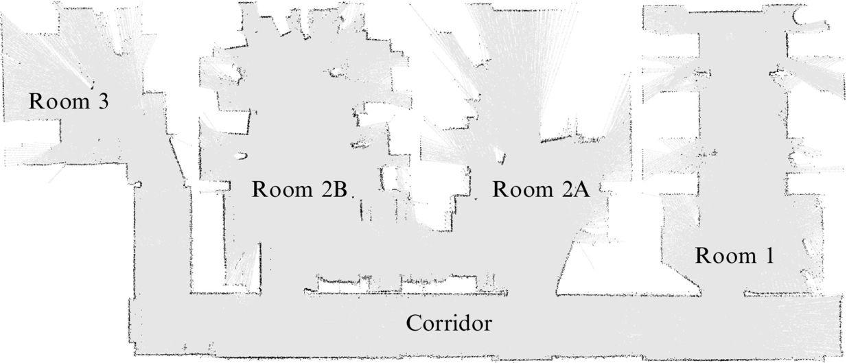
An example of the map that was obtained from a combination of LRF scanner measurements and odometry data using the SLAM algorithm is shown in Fig. 5.33.
SLAM is the one of the basic approaches that is used in wheeled mobile robotics. Some of the common challenges in localization of mobile robots are the following:
• Pose initialization of the mobile robot at start-up cannot be determined with high probability. If the initial pose is not known, the global localization problem needs to be solved.
• The problem of robot kidnapping occurs when the real mobile robot pose in the environment changes instantly while the mobile robot is in operation (e.g., the mobile robot is transported to a new location or it is turned on at a different location as it has been turned off). Robust localization algorithms should be able to recover and estimate the real robot pose.
• Ensuring an appropriate pose estimate during the movement of the mobile robot. For this purpose, odometry data and measurements from absolute sensors are used.
The most commonly used algorithms for solving the SLAM problem are the extended Kalman filter, Bayesian filter, and particle filter (see Chapter 6).
5.4 Sensors
This section provides a brief description of the main sensors used in wheeled mobile robotics, their characteristics, and classification.
5.4.1 Sensor Characteristics
Sensors’ operation, their quality, and properties are characterized in different ways. The most common characteristics are as follows:
• Range defines the upper (ymax) and the lower limit (ymax) of the applied quantity that can be measured. The upper and lower limits are usually not symmetrical. Sensors should be used in the specified range, and exceeding this range may result in sensor damage.
• Dynamic range is the total range from the minimum to maximum range value. It can be given as a difference Rdyn = ymax − ymin or more commonly as a ratio (in decibels) ![]() where A = 10 for power-related measurements and A = 20 for the rest.
where A = 10 for power-related measurements and A = 20 for the rest.
• Resolution is the smallest change of the measured quantity that can be detected by the sensor. If the sensor has an analog-to-digital converter then sensor resolution is usually the resolution of the converter (e.g., for 10 bit A/D and 5 V sensor range the resolution is ![]() ).
).
• Sensitivity is the sensor output change per unit of the quantity being measured (e.g., distance sensor measures distance which is given as the voltage on the sensor output). Sensitivity can be constant over the whole sensor range (linear) or it can vary (nonlinearity).
• Linearity of the sensor is the sensor property where the sensor output is linearly dependent (proportional) from the measured quantity over the entire range. A linear sensor has constant sensitivity in the whole range.
• Hysteresis refers to the property that the sensor output trajectory (or its dependence on input) is different for situations when sensor input is increasing or decreasing.
• Bandwidth refers to the frequency by which the sensor can provide measurements (given Hz). It is the highest frequency (sampling rate) at which only 70.7% of the true value is measured.
• Accuracy is defined by the expected measurement error that is the difference between measured (m) and true value (v). Accuracy is computed from the relative measurement error using ![]() .
.
• Precision is degree of reproducibility of the sensor measurement at the same true value of quantity being measured. Real sensor output produces a range of values when the same true value is being measured many times. Precision is related to the variance of the measurement.
• Systematic error or deterministic error is caused by some factors that can be predicted or modeled (bias, temperature drift, sensor calibration, distortion caused by lens of the camera, etc.).
• Random error or nondeterministic error is unpredictable and can only be described by a probability density function (e.g., normal distribution). This error is usually called noise and is usually characterized by the SNR.
5.4.2 Sensor Classifications
Wheeled mobile robots can measure the internal state using proprioceptive sensors or the external state of the environment using exteroceptive sensors. Examples of proprioceptive measurements include robot position and orientation, wheel or steering mechanism rotation, angular velocity of the wheels, state of the accumulators, temperature, and current on the motor. Examples of exteroceptive measurements, on the other hand, include distance to obstacles, image captured by camera, microphone, compass, GNSS, and others.
Sensors used for a environment detection are used for path planning purposes, obstacle detection, environment mapping, etc. Those sensors are active if they emit energy (electromagnetic radiation) in the environment and measures received response from environment (LRF, ultrasonic sensors, camera with integrated illumination, etc.). Sensors are passive if they receive energy that is already part of the environment. Passive sensors are therefore all sensors that are not active (camera without illumination, compass, gyroscope, accelerometer, etc.).
In Table 5.1 the most common sensors in mobile robotics are listed according to their usage. Additionally a brief description of their application, purpose (proprioception [PC] or exteroception [EC]), and emitted energy (active A or passive P) is included.
Table 5.1
Classification of sensors in mobile robotics according to their application, purpose (proprioception [PC]/exteroception [EC]), and emitted energy (active [A]/passive [P])
| Classification | Applicability | Sensors | PC/EC | A/P |
| Tactile and haptic | Collision detection, security shutdown, closeness, wheel or motor rotation | Contact switches | EC | P |
| Bumpers | EC | P | ||
| Optical barriers | EC | A | ||
| Proximity sensors | EC | P/A | ||
| Contact arrays | EC | P | ||
| Axis | Wheel or motor rotation, joint orientation, localization by odometry | Incremental encoders | PC | A |
| Absolute encoders | PC | A | ||
| Potentiometer | PC | P | ||
| Tachogenerators | PC | P | ||
| Heading | Orientation in reference frame, localization, inertial navigation | Gyroscope | PC | P |
| Magnetometer | EC | P | ||
| Compass | EC | P | ||
| Inclinometer | EC | P | ||
| Speed | Inertial navigation | Accelerometer | EC | P |
| Doppler radar | EC | A | ||
| Camera | EC | P | ||
| Beacon | Object tracking, localization | IR beacons | EC | A |
| WiFi transmitters | EC | A | ||
| RF beacons | EC | A | ||
| Ultrasound beacons | EC | A | ||
| GNSS | EC | A/P | ||
| Ranging | Measure distance to obstacle, time-of-flight (TOF), localization | Ultrasound sensor | EC | A |
| Laser range finder | EC | A | ||
| Camera | EC | P/A | ||
| Machine-vision- | Identification | Camera | EC | P/A |
| based | Object recognition | TOF camera | EC | A |
| Object tracking | Stereo camera | EC | P/A | |
| Localization | RFID | EC | A | |
| Segmentation | Radar | EC | A | |
| Optical triangulation | EC | A |
