
Project Examples for Laboratory Practice
Abstract
This chapter contains some practical examples that can be used to prepare laboratory practice or to consolidate learned theory. There are eight different examples that apply the book theory to some practical applications. In several different hardware setups implementation of wheeled mobile robot localization based on Bayesian, Kalman, and particle filter is presented. There are some examples that present application of different control algorithms, also some that have been used in the FIRA Micro Robot World Cup Soccer Tournament. One example covers some basic visual control approaches and another example focuses on implementation of path planning in an indoor environment.
Keywords
Odometry; Localization; Mapping; State estimation; Path planning; Control; Obstacle avoidance; Autonomous navigation; Visual servoing
8.1 Introduction
This chapter contains several examples that demonstrate the applications of the methods presented in the book for solving different problems in autonomous mobile robotics. This chapter contains several practical examples that demonstrate somewhat more involved applications of the methods presented in the book on wheeled mobile robots. Each example is about a specific problem and/or particular problem solving methodology. Every example is structured as follows: at the beginning is a description of the problem, then one of the possible solutions is presented in more detail, and at the end some experimental results are shown. The examples are given in a way that the interested reader should be able to implement the presented algorithms in a simulation environment and also on a real wheeled mobile system. Therefore, the experiments are designed in a way that the proposed methods can be implemented on some common educational and research wheeled mobile robots. Although every example contains the recommended robotic platform for algorithm implementation, other robotic platforms could also be considered. Wheeled mobile robots used in the examples to obtain the real-world experimental results were the following: vacuum cleaning mobile robot iRobot Roomba, research mobile robot Pioneer 3-AT with SICK laser range-finder, Lego Mindstorms EV3 set, and soccer robots that are normally used in FIRA Micro Robot World Cup Soccer Tournaments.
The examples are intended to guide the reader through the process of solving different problems that occur in implementation of autonomous mobile robots. The examples should motivate the reader to implement the proposed solutions in a simulation environment and/or real mobile robots. Since most of the examples can be applied to various affordable mobile robots, the examples should give the reader enough knowledge to repeat the experiments on the same robotic platform or modify the example for a particular custom mobile robot. The examples could be used as a basis for preparation of lab practice in various autonomous mobile robotic courses.
8.2 Localization Based on Bayesian Filter Within a Network of Paths and Crossroads
8.2.1 Introduction
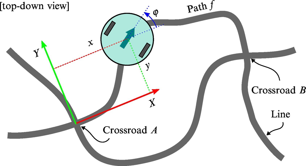
This demonstration exercise shows how the Bayesian filter can be applied for localization of a wheeled mobile system within a known map of the environment. The exercise also covers some basic principles of line-following, map building, and navigation within the map. Consider that the map of the environment is represented with lines that are drawn on the ground and represent the paths that the mobile system can drive on. The intersection of lines represent crossroads where the mobile system can select different paths. For the sake of simplicity, only two lines can intersect in a single crossroad and there should be some minimum distance between every pair of crossroads. The goal of the exercise is to develop a mobile system that is able to localize within the network of interconnected lines (map) and navigate between arbitrary locations in the map. The algorithms should be implemented on a two-wheeled differentially driven mobile platform that is equipped with an infrared light reflection sensor, which is used for detection of a line that is drawn on the ground. Through the rest of this exercise we will consider that a Roomba mobile system is used for implementation. However, any other mobile system that is capable of line following and crossroad detection could also be used. Although this is only an exercise, an appropriate solution to the problem has some practical applications in real-life environments, such as automated warehouses and distribution centers, where wheeled mobile platforms are used to transfer objects (parcels) between different stations.
The exercise is composed of several sections, where in every section a small subsystem is developed that is required for implementation of the complete localization solution. The first section is devoted to implementation of line following and crossroad selection control algorithm. The second section is about implementation of the odometry algorithm. In the third section an approach for map building is presented, and the final section presents the method for localization within the map.
8.2.2 Line Following
The first task consists of implementation of a control algorithm for line following and crossroad detection. In our case, we consider using an infrared light sensor for line detection. Consider which other sensors do you think could also be used for line detection, and how.
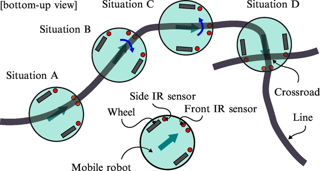
The bottom of the iRobot Roomba (series 500) mobile system is equipped with four light sensors that are normally used for detection of holes (cliffs) in the ground. The front two light sensors can be used for line detection and the side sensors for crossroad detection. Fig. 8.1 shows how the IR sensors can be used for line tracking (front sensors) and for crossroad detection (side sensors).
8.2.3 Odometry
Observing the rotation of the wheels, the position of the mobile platform in the environment can be tracked using the approach that is known as odometry. Assume that the rotation of a wheel is measured with an encoder with counter γ. Let us assume that the value of the encoder counter is increasing when the wheel rotates in a forward direction and the value of the counter is decreasing when the wheel rotates in the opposite direction. The temporal difference of counter values Δγ(k) = γ(k) − γ(k − 1) is proportional to the relative rotation of the wheel. Based on the temporal difference of counter values of the left ΔγL(k) and right ΔγR(k) encoder, the relative rotations of the left ΔφL(k) and right ΔφR(k) wheel can be calculated, respectively:

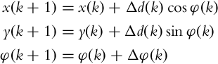
The pose (x(k), y(k), φ(k)) of the mobile system can be approximated with a discrete solution of the direct kinematic model of the wheeled mobile system, using the Euler integration method of first differences:
The relative distance Δd(k) and relative rotation Δφ(k) of the mobile system can be determined from relative rotations of the wheels:

where L is the distance between the wheels and r is the radius of the wheels.
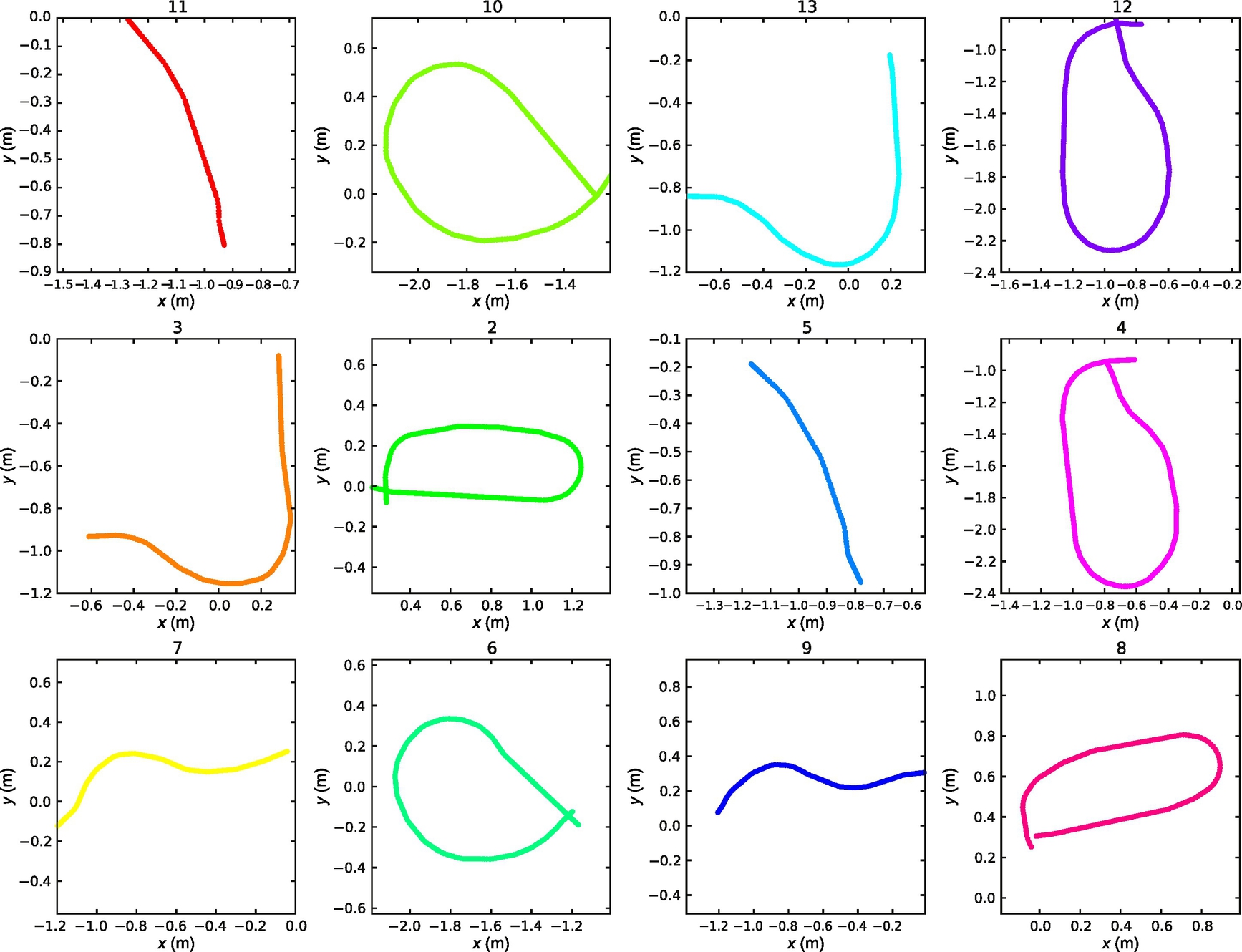
In Fig. 8.2 an example of a path obtained by odometry is shown.

8.2.4 Map Building
In this section a method for a semiautomated supervised method of map building is presented. The lines drawn on the ground intersect at several crossroads, for example, in Fig. 8.3. For the sake of simplicity, we assume that all the crossroads connect four paths and that all paths are connected to crossroads at both ends. The shapes of the paths between the crossroads are assumed to be arbitrary. We label all the K crossroads with a set ![]() and all the P direct paths between the crossroads with a set
and all the P direct paths between the crossroads with a set ![]() . Every path is given a dominant direction in a way that if direction of path pi is from crossroad Kj to Kl, the path
. Every path is given a dominant direction in a way that if direction of path pi is from crossroad Kj to Kl, the path ![]() is in the opposite direction, that is from crossroad Kl to Kj. The nondominant paths are gathered in a set
is in the opposite direction, that is from crossroad Kl to Kj. The nondominant paths are gathered in a set ![]() . In the case in Fig. 8.3 there are K = 3 crossroads, which are labeled with a set
. In the case in Fig. 8.3 there are K = 3 crossroads, which are labeled with a set ![]() , and P = 6 direct paths, which are labeled with a set
, and P = 6 direct paths, which are labeled with a set ![]() . The spatial representation of the crossroads and paths can therefore be represented as a graph, like shown on the right-hand side of Fig. 8.3. When redrawing spatial representation of the map into a graph form, the connections (paths) into nodes (crossroads) should be drawn in the same order as in the real map. This is required to be able to determine which path in a crossroad is on the left, right, and straight ahead if the mobile system enters the crossroad from an arbitrary path. An alternative is to save the order of paths in a crossroad in a table, like it is shown in Table 8.1, where the locations of the paths in a crossroad can be determined from the ordered list of paths. The ending nodes of all the direct connections can also be represented in the form of a table (Table 8.2), where the order of nodes is important to distinguish between dominant and nondominant path direction. Therefore the entire map can be represented in a form of a graph or an equivalent table; these data structures are simple to implement in a computer’s memory.
. The spatial representation of the crossroads and paths can therefore be represented as a graph, like shown on the right-hand side of Fig. 8.3. When redrawing spatial representation of the map into a graph form, the connections (paths) into nodes (crossroads) should be drawn in the same order as in the real map. This is required to be able to determine which path in a crossroad is on the left, right, and straight ahead if the mobile system enters the crossroad from an arbitrary path. An alternative is to save the order of paths in a crossroad in a table, like it is shown in Table 8.1, where the locations of the paths in a crossroad can be determined from the ordered list of paths. The ending nodes of all the direct connections can also be represented in the form of a table (Table 8.2), where the order of nodes is important to distinguish between dominant and nondominant path direction. Therefore the entire map can be represented in a form of a graph or an equivalent table; these data structures are simple to implement in a computer’s memory.
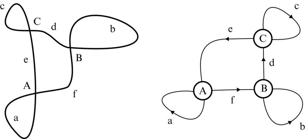
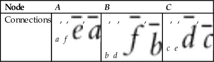
Table 8.2
Ending nodes (crossroads) of the connections (paths)
| Connection | a | b | c | d | e | f |
| Nodes | A, A | B, B | C, C | B, C | C, A | A, B |

With the current representation of the map in a form of a graph (or table) the spatial relations between the crossroads (nodes) are lost as are lost the shapes of the paths (connections). Since we assume all the crossroads are of the same shape (four paths perpendicular to adjacent paths), the entire map can be built when the shapes of all the direct paths between crossroads are known. The shapes of all the direct paths can be recorded with the process of odometry (Fig. 8.4). Although the process of odometry has some obvious disadvantages, it should be sufficient to determine the approximate shape of the path between two nodes. Therefore, if the shapes of at least some paths are different enough, it should be possible to determine the location of the mobile system within a map, based on the stored map data (graph representation of the map and shapes of all the direct paths). A map of the environment is represented with a set of crossroads ![]() , a set of paths
, a set of paths ![]() , and recorded shapes of the paths with the process of odometry. In the process of map building all this information needs to be written into appropriate data structures and saved in a nonvolatile memory area.
, and recorded shapes of the paths with the process of odometry. In the process of map building all this information needs to be written into appropriate data structures and saved in a nonvolatile memory area.
Exercise
Record the shapes of all the direct paths with the odometry (Fig. 8.5) as follows: put the mobile system at the beginning of path in the starting crossroad, let the mobile system follow the line until the next (ending) crossroad, save the recorded shape of the path, and repeat for all the other paths. The map of the environment should be saved into a nonvolatile memory area (e.g., as a text file on a hard disk).
8.2.5 Localization
In this section an algorithm for localization within a map built in the previous section is presented. The goal of localization is to determine the current path followed by the mobile system, the direction of driving (from the starting node to the ending node), and the distance from the starting or ending node.
Assume the mobile system is traveling along the paths by line following and randomly choosing the next path at the crossroads. Comparing the current odometry data with the odometry data stored in a map, the mobile system should be able to localize within the map. The basic concept of localization is as follows. The current odometry data from paths between crossroads is compared to all the odometry data stored in a map. Based on predefined goodness of fit, the probabilities of all the paths are calculated. Once the probability of a specific path is significantly larger than the probabilities of all the other paths, the location of the mobile system is considered to be known (with some level of probability).
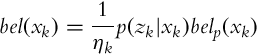
The localization problem can be solved in a framework of Bayesian filter. For the sake of implementation simplicity, assume that the localization algorithm is executed only once the mobile system reaches a new crossroads, just before the next path is selected. The location of the mobile system is therefore known, if it is known from which path the mobile system reached the crossroad. Since every path has two directions, we need to consider the probabilities of all the direct paths in both directions. For every path ![]() the following belief functions need to be calculated:
the following belief functions need to be calculated:

where ![]() .
.
Assume that the localization algorithm is first executed when we arrive at the first crossroad. In the initial step the location of the mobile system is unknown; therefore, all the paths have the same level of probability. The mobile system therefore leaves the crossroad at an arbitrary direction based on the given control action (go forward, left, right, or back). The path selection control algorithm is assumed to select the desired path with some level of probability. All the exiting paths in a crossroad can be marked with labels s1, s2, s3, and s4 as shown in Fig. 8.6. The probabilities of selecting the path s1 if the current path is one of the paths ![]() ,
, ![]() ,
, ![]() , and
, and ![]() need to be determined for all the possible control actions. For example, for control action forward the probabilities could be as follows:
need to be determined for all the possible control actions. For example, for control action forward the probabilities could be as follows:


Exercise
Based on the robustness of the path selection algorithm determine the probabilities p(xk|xk−1, uk) of selecting path Xk = s1 if the current path is one of the paths ![]() ,
, ![]() ,
, ![]() ,
, ![]() for all the possible control actions Uk ∈{forward, left, right, back}.
for all the possible control actions Uk ∈{forward, left, right, back}.
Since the crossroads are symmetric, the following relations are assumed to hold:

For all the exiting paths a table of corresponding entering paths can be written in a table form that proves to be convenient when implementing the localization algorithm (see Table 8.3).
Table 8.3
Entering paths for all the exit paths from example in Fig. 8.3
| s1 | a | b | c | d | e | f | ||||||
| a | b | c | d | e | f | |||||||
| a | b | c | e | f | d | |||||||
| e | f | d | b | c | a | |||||||
| f | d | e | c | a | b |

The mobile system then leaves the crossroad, follows the line and records the odometry data until the next crossroad is detected. Once the mobile system arrives in the next crossroad the recorded odometry between the previous and current crossroad is compared to all the odometry data stored in a map. To determine the probability p(zk|xk) some distance measure for comparing the shapes of odometry data needs to be defined. The most probable path is therefore the path with the smallest distance value.
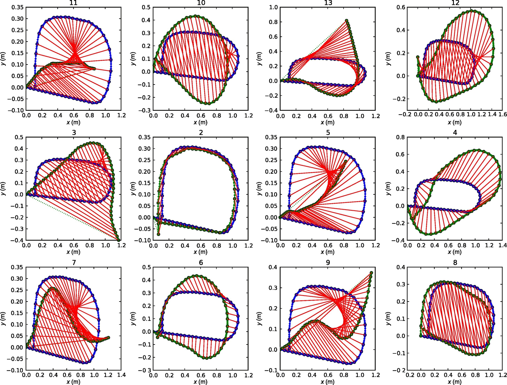
In Fig. 8.7 an idea for definition of path comparison measure is shown. Different distance measures can be defined, for example: ![]() or
or ![]() , where m is the number of comparison points (the measures are also shown in Fig. 8.8).
, where m is the number of comparison points (the measures are also shown in Fig. 8.8).

The belief function in Eq. (8.5) can now be updated. The evolution of belief distribution is shown in Fig. 8.9. In the initial step the probabilities of all the paths are equal (Fig. 8.9A). When the mobile system travels the first path between two crossroads, the probability of paths based on measured data is calculated (Fig. 8.9B) and the belief function is updated (Fig. 8.9C). After several steps, when the mobile system visits several crossroads the most probable path according to the belief function should be the real path.

8.3 Localization Based on Extended Kalman Filter Using Indoor Global Positioning System and Odometry
8.3.1 Introduction
Mobile robots are normally required to be able to localize in the environment in order to perform some desired tasks autonomously. In order to give a mobile system the localization capability the mobile system must be equipped with an appropriate sensor that can determine the position of the mobile system with respect to the external (global) coordinate frame. This can be achieved in various ways. In this exercise a localization approach that acquires the position from an external measurement system is considered. In an outdoor environment the global position can be determined with a global navigation satellite system (GNSS) that is nowadays available all over the world (the accuracy may vary). Since the GNSS does not work in an indoor environment, some special localization systems have been developed for indoor localization. Some are based on measuring wireless network signal strength or time of flight between several static transmission points, while others use image-based object tracking technology. Global positioning systems normally measure only the position but not also the orientation of the tracked object. However, for implementation of autonomous navigation, the wheeled mobile system must be aware of its position and orientation.
8.3.2 Experimental Setup
This exercise covers how the pose of the wheeled mobile robot in space can be estimated based on odometry data and measurement of the position of the mobile system within the environment. The considered setup (Fig. 8.10) consists of a wheeled mobile system equipped with wheel encoders and a measurement unit that is able to determine the position of the tag (mounted on top of a mobile system) with respect to some anchor nodes with fixed and known positions in the environment. A mobile robot with differential drive (Section 2.2.1) will be used; however, the presented approach can be used on any other wheeled mobile drive. The experimental setup consists of a wheeled mobile system that has rotation encoders on each wheel.
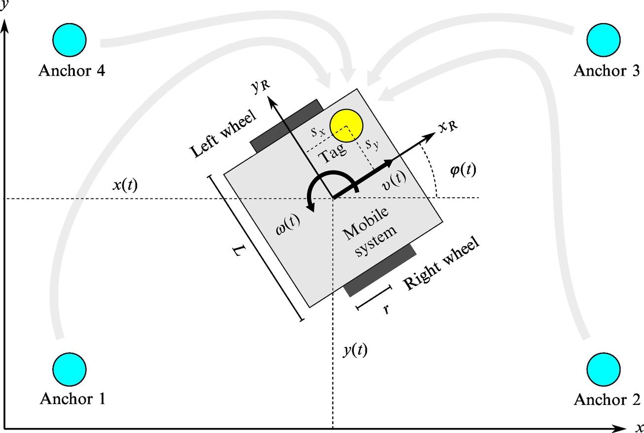
Based on the encoder readings, an odometry approach can be used for estimation of mobile system pose. Since the pose obtained by odometry is susceptible to drift, the pose estimate must be corrected by external position measurements. The position of the mobile system is obtained using an indoor positioning system, but this measurement system has limited precision. This is a sensor fusion problem, that for the given setup can be solved in the framework of an extended Kalman filter (EKF). Once the localization algorithm is implemented and tuned, the mobile system can be extended with the capability of autonomous navigation between desired locations within the environment.
8.3.3 Extended Kalman Filter
Here an extended Kalman filter (EKF) is considered for solving the mobile system localization problem. The EKF (Section 6.5.2) is an extension of a conventional Kalman filter to nonlinear systems with linear approximation of covariance matrices. The algorithm has a two-step structure, prediction of the states based on the current action (Eq. 6.38), and correction of the predicted states when a new system output measurement becomes available (Eq. 6.39). To implement the EKF, a model of the system and model of the noise must be given. The nonlinear model of the system (6.37) has to be linearized around the current estimated state in order to obtain the matrices (6.40)–(6.42). The most challenging part in implementation of the EKF is an appropriate modeling of system kinematics and noise, which come as a result from various processes. Noise is normally time or state dependent, and is hard to measure and estimate.
Prediction Step
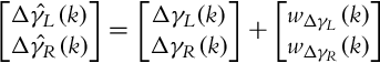
Let us develop a kinematic odometry model that takes into account system uncertainties. The robot wheels are equipped with encoders γL and γR that track the orientation of left and right wheel, respectively. The relative encoder readings of the left and right wheel, Δγ{L, R}(k) = γ{L, R}(k) − γ{L, R}(k − 1), are assumed to be proportional to the angular velocities of the wheels, ![]() . Let us assume that the readings of rotation encoders of each wheel, γL and γR, are disturbed by additive white noise
. Let us assume that the readings of rotation encoders of each wheel, γL and γR, are disturbed by additive white noise ![]() . Distinguish between angular velocities, annotated with Greek letter ω, and noise, annotated with letter w. This noise is assumed to encapsulate not only the measurement noise, but also the effects of all the noises that are due to different sources, including wheel slippage. The encoder readings
. Distinguish between angular velocities, annotated with Greek letter ω, and noise, annotated with letter w. This noise is assumed to encapsulate not only the measurement noise, but also the effects of all the noises that are due to different sources, including wheel slippage. The encoder readings ![]() are therefore assumed to be related to the true encoder values Δγ{L, R}(k) as follows:
are therefore assumed to be related to the true encoder values Δγ{L, R}(k) as follows:
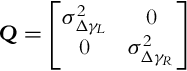
Assume that the distribution of noise is normal (Gaussian) with zero mean, ![]() . For the application of EKF the distribution of the noise need not be normally distributed, but the noise should be unbiased. The noise covariance matrix Q is assumed to be diagonal, since no cross-correlation between the wheel noise is assumed:
. For the application of EKF the distribution of the noise need not be normally distributed, but the noise should be unbiased. The noise covariance matrix Q is assumed to be diagonal, since no cross-correlation between the wheel noise is assumed:
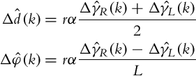
Based on the relative encoder readings, ![]() , the relative longitudinal traveled distance
, the relative longitudinal traveled distance ![]() and relative rotation
and relative rotation ![]() of the wheeled mobile system can be determined:
of the wheeled mobile system can be determined:
The discrete kinematic model of a differential drive (Eq. 2.3) can be written in the following form:

Since the wheels are disturbed by noise, the estimated pose of the wheeled mobile system using the recursive estimation approach (Eq. 8.11) is susceptible to drift.
The parameters in the odometry algorithm (T, r, L, and α) could all be measured. However, to implement the odometry algorithm only the parameters Trα and L need to be known. These two parameters can be obtained with an appropriate calibration procedure. For example, the mobile system can be drawn along a circular arc, and the two parameters Trα and L can be obtained from two equations (8.10) if the length and relative rotation of the circular arc are known.
The kinematic model of wheel odometry (Eq. 8.11) without noise can be used to make predictions about the mobile system pose and can therefore be used in the prediction step of the EKF. In the prediction step of the EKF, the new state of the system (mobile system pose) is predicted based on the state estimate from the previous time step (using the nonlinear system model, Eq. 8.11 without noise in our case), and also the new covariance matrices are calculated (from linearization of the system around the previous estimate).
The Jacobian matrices required in the prediction step of the EKF are determined from Eqs. (6.40), (6.41), as follows:
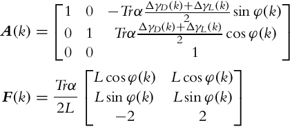
Taking into account the input noise covariance matrix (8.9), the matrix FQFT that occurs in Eq. (6.38) is then

Considering that the variance of all the diagonal elements in Eq. (8.9) are equal to each other, the last term in Eq. (8.13) is zero.
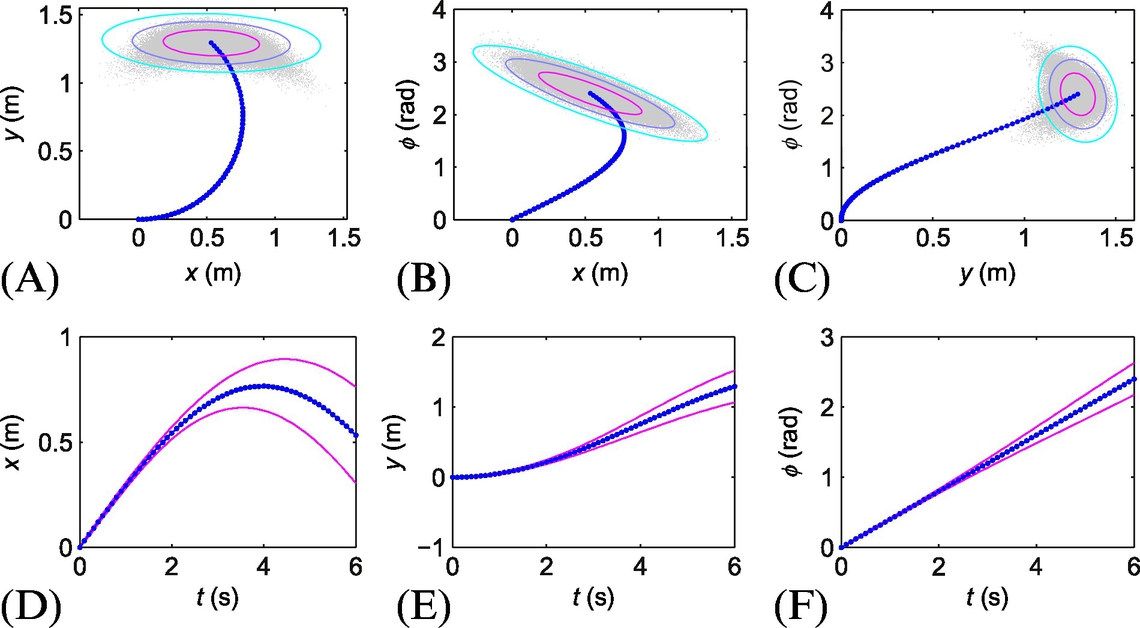
Fig. 8.11 shows simulation results, where constant input velocities were applied to the robot. The bottom row in Fig. 8.11 shows time evolution of the state predictions with state error covariance boundaries of one standard deviation. The top row in Fig. 8.11 shows the predicted path (2D projections of the generalized robot coordinates) and contours of the projected state error covariance matrix in the final state. The plots in the top row also show the predicted clouds of final state after many repetitions of the model simulation with added simulated noise. Notice the dissimilar shape between the final state clouds and the estimated error covariance matrices (ellipses).
Exercise
Assume that a white noise is independently added to the signals Δd and Δφ instead of the signals ΔγL and ΔγR, that is, ![]() and
and ![]() . Calculate the new state error covariance equations and modify the state prediction algorithm. Notice that, in this case, the values in covariance matrix Q have different meanings.
. Calculate the new state error covariance equations and modify the state prediction algorithm. Notice that, in this case, the values in covariance matrix Q have different meanings.
Correction Step
Once a new measurement of the system output state is available, a current state estimate can be updated in the correction step (6.39) of the EKF. To be able to update the system states a model of the system output needs to be determined.

The measurement noise v = [vxvy] can be modeled as white noise with zero mean and Gaussian distribution, ![]() .
.
The Jacobian matrix C(k) is determined from the nonlinear measurement model (8.14), as follows:

Normally we can assume a diagonal measurement noise covariance matrix:

where ![]() and
and ![]() are the measurement noise variances along the x and y directions, respectively, and are normally equal to each other. If there is significant correlation between noise signals vx(k) and vy(k) a general form of the noise covariance matrix R should be used. In a special case, when the sensor is mounted in the rotation center of the mobile system (sx = 0 and sy = 0) the model (8.14) simplifies, the last column in Jacobian matrix C(k) becomes zero, and therefore all the measurement Jacobian matrices become constant unity matrices.
are the measurement noise variances along the x and y directions, respectively, and are normally equal to each other. If there is significant correlation between noise signals vx(k) and vy(k) a general form of the noise covariance matrix R should be used. In a special case, when the sensor is mounted in the rotation center of the mobile system (sx = 0 and sy = 0) the model (8.14) simplifies, the last column in Jacobian matrix C(k) becomes zero, and therefore all the measurement Jacobian matrices become constant unity matrices.
Accurate noise modeling is one of the most crucial parts in implementation of EKF. Assume that the variance of the noise on each wheel is dependent on the speed of the wheel, so that the following relation holds ![]() that yields [1]:
that yields [1]:

In this noise model, the parameter δ defines the proportion of the noise with respect to the wheel velocity.
An example of the estimated path is shown in Fig. 8.12. Although the initial pose estimate is wrong, the localization algorithm converges to true mobile robot pose. The filter also estimates mobile robot heading, which cannot be obtained from the global positioning system directly. The heading could be determined from differentiation of position measurements, but in the presence of noise this is extremely unreliable without appropriate signal prefiltering, which introduces lag. A Kalman filtering approach as shown in this example is therefore preferred.
8.4 Particle-Filter-Based Localization in a Pattern of Colored Tiles
8.4.1 Introduction
Localization is one of the most fundamental problems in wheeled autonomous robotics. It is normally solved in the framework of Bayesian filter. Among various filtering approaches (Kalman filter, EKF, UKF, etc.) particle filter [2] is gaining more and more attention. In this exercise it will be shown how the particle filter can be used to solve the localization of a wheeled mobile robot on a plane made of colored tiles.
8.4.2 Experimental Setup
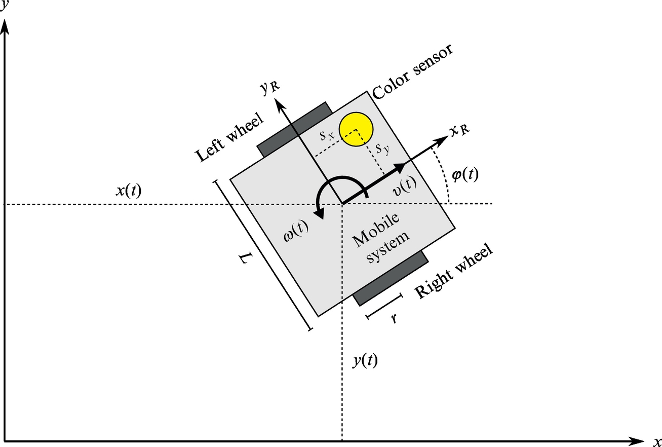
The wheeled mobile robot is equipped with wheel encoders and a color sensor that can determine the color of the surface below the robot (Fig. 8.13). The mobile robot is assumed to have differential drive with axle length L and wheel radius r. The mounting of the color sensor on the robot is displaced from the robot’s center of rotation for sx and sy in robot longitudinal and lateral direction, respectively. The ground plane consists of square, colored tiles of equal sizes that cover a rectangular area of ![]() times
times ![]() tiles. The mobile robot is only allowed to move inside the area of tiles that is enclosed with a wall boundary. There are
tiles. The mobile robot is only allowed to move inside the area of tiles that is enclosed with a wall boundary. There are ![]() distinct colors of the tiles. The arrangement of the colored tiles on the ground (i.e., the map) is assumed to be known. Fig. 8.14 shows a map of the environment with dimensions of 180 × 100 cm2, where M = 10, N = 18, and L = 6. The considered setup can be built with the elements provided in the Lego Mindstorms EV3 kit, which is also used in this example to obtain some real-world data.
distinct colors of the tiles. The arrangement of the colored tiles on the ground (i.e., the map) is assumed to be known. Fig. 8.14 shows a map of the environment with dimensions of 180 × 100 cm2, where M = 10, N = 18, and L = 6. The considered setup can be built with the elements provided in the Lego Mindstorms EV3 kit, which is also used in this example to obtain some real-world data.

8.4.3 Manual Control
This exercise is about implementation of the localization algorithm. Therefore, it suffices to drive the mobile robot only manually, but once the localization algorithm is implemented and evaluated also some automatic driving control algorithm can be developed.
8.4.4 Wheel Odometry
Wheel odometry is one of the basic localization approaches that can be used to estimate mobile robot pose, given a known initial pose. It is known that the approach is susceptible to drift, due to wheel slippage, but the error over short distances is normally relatively small. The drift can be eliminated if additional information about position is available; in this case a color sensor is considered. Estimated motion based on the internal kinematic model of the wheeled mobile robot is normally used in the prediction step of every localization algorithm that is based on Bayesian filtering, including the particle filter. Wheel odometry is normally implemented based on incremental encoder measurements (motors in the Lego Mindstorms EV3 kit are all equipped with encoders). In order to fine tune the parameters (wheel radius and axle length) of the odometry algorithm to a particular wheeled mobile system design, an appropriate calibration is normally employed.
8.4.5 Color Sensor Calibration
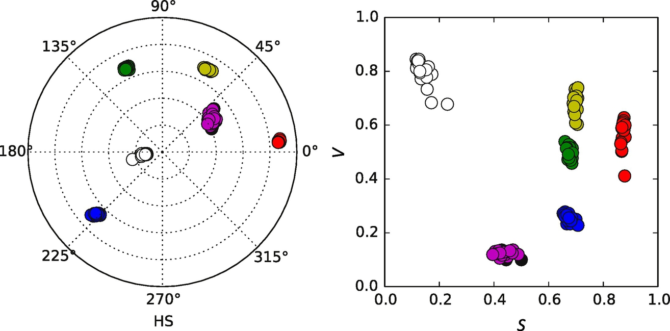
The odometry drifting can be eliminated with the readings of the tile color below the wheeled mobile robot, since the arrangement of the colored tiles (map of the environment) is assumed to be known. For detection of the surface color a color sensor needs to be used (Mindstorms EV3 kit contains a color sensor). Suppose that a single color sensor measurement is encoded as RGB triple, that is, value of red, green, and blue components in the RGB color space. The color sensor is required to distinguish between C different colors of the tiles that make up the ground surface. For this purpose the raw sensor readings (RGB values) need to be classified into one of the C color classes (an additional class can be defined for any other color. The color sensor needs to be calibrated for the particular mounting of the sensor on the mobile robot and the ground surface. Robust color classification is normally simpler to achieve in HSV (hue-saturation-value) that in the RGB color space. Therefore RGB to HSV color conversion (Eq. 5.87) needs to be used. Fig. 8.15 shows that color readings of six different colored tiles are clearly separable in the HSV color space.
8.4.6 Particle Filter
Color sensor measurements and odometry data provide partial information about the global pose of the wheeled mobile robot. A particle filter can be used in order to join information from different sources to obtain a better estimate about the robot pose. A color sensor alone cannot provide information about the mobile robot heading directly, but in the framework of a particle filter it can be used to remove the odometry drift and enable global localization, that is, the initial pose of the mobile robot need not be known in advance. The basic idea behind the particle filter is that the probability distribution of the state estimate is approximated with a set of particles. In this case particles represent hypotheses about the pose of the wheeled mobile robot. The algorithms consists of several steps: particle initialization, prediction, importance resampling, and evaluation of the most plausible wheeled mobile robot pose based on particle distribution. The steps of the algorithm are depicted in Fig. 8.16 (working area is smaller than in Fig. 8.14 to improve visibility).

In the initial step of particle filter initial population of ![]() , the particles need to be determined. In the particular case each particle represents a hypothesis about the wheeled robot pose, that is, the ith particle represents the possible robot position and heading
, the particles need to be determined. In the particular case each particle represents a hypothesis about the wheeled robot pose, that is, the ith particle represents the possible robot position and heading ![]() . The particles should be distributed in accordance with the initial probability distribution of the wheeled robot pose. In a case that the initial robot pose is not known, a uniform distribution can be used, that is, the particles should be spread uniformly over the entire state space. Fig. 8.16A shows the initial uniform distribution of particles.
. The particles should be distributed in accordance with the initial probability distribution of the wheeled robot pose. In a case that the initial robot pose is not known, a uniform distribution can be used, that is, the particles should be spread uniformly over the entire state space. Fig. 8.16A shows the initial uniform distribution of particles.
The wheeled mobile robot can then make a move. The first step of the algorithm is prediction of the particles. Each particle is updated based on the assumed change in mobile robot pose. This is normally made according to the estimated pose change based on odometry data Δd(k) and Δφ(k), that is, for the ith particle the update equations are (a simple Euler integration of the differential drive kinematic model is used) the following:
To the predicted pose estimate of each particle a randomly generated noise with appropriate distribution can be added to model disturbances, for example, wheel slippage. The predicted distribution of the particles after prediction of the particles is shown in Fig. 8.16B.
The color of the tile below the mobile robot is then measured. For the sake of simplicity assume that the color sensor is positioned in the rotation center of the mobile robot (sx = 0 and sy = 0). Sensor measurement is used to determine the importance of each particle based on comparison of the measured color with the tile color below the particular particle. The particles that agree with the measurement are given a high importance score and the others are given a small score. The score of a particular particle can be determined according to the distance to the nearest tile that is of the same color as measured by the sensor.
Assigned importance to each particle is used in the particle resampling step. Particles are randomly sampled in a way that the probability of selecting a particular particle from a set is proportional of the particle importance score. Therefore, the particles with larger importance score are expected to be selected more times. The updated distribution of the particles after the resampling step is shown in Fig. 8.16C.
The final step consists of particle evaluation in order to estimate the wheeled mobile robot pose from the distribution of the particles. This can be made in various ways, as a (weighted) average of all the particles or based on the probabilities of the particles. The estimated pose is shown in Fig. 8.16D.
The mobile robot then makes another move, and in the next time-step the algorithm proceeds to the next prediction step. Fig. 8.16E–G shows the estimated pose after three more particle filter iterations, and Fig. 8.16H shows the estimated pose after several more iterations. In the demonstrated case the particle filter was updated only when the value of the color measurement changed. More details about the particle filter algorithm can be found in Section 6.6.
8.5 Control of Vehicles in a Linear Formation
8.5.1 Introduction
Future intelligent transportation systems are hard to imagine without autonomous wheeled vehicles. One important application is an automated platoon of vehicles on highways that can drive autonomously in so-called virtual train formation. Vehicles in this platoon should precisely and safely follow their leader vehicles with minimal safety distance required. This would increase vehicle density on highways, avoid traffic jams, and increase safety.
In this exercise a control algorithm of mobile robots driving in linear formation will be designed. To obtain automated driving formation precise sensor systems are required, measuring global information such as GPS or relative information such as distance and bearing or both. Here we will implement a decentralized control strategy relying only on a relative sensor—laser range finder (LRF). Suppose that each vehicle has LRF to measure the distance and the azimuth of its leading vehicle. This information is then used to record and track the path of the leader vehicle. The leading vehicle path is recorded in local coordinates of the follower using odometry and LRF measurement (distance D and azimuth α) as shown in Fig. 8.17.

The follower vehicles than follow the estimated paths of their leader vehicles using trajectory tracking control approaches as presented in Section 3.3. It is well known that robot localization using odometry is pruned to accumulation of different errors (e.g., wheel sleep, sensor and actuator noise, and the like). Odometry is therefore usable only for short-term localization. As illustrated a latter absolute pose error made using odometry is not significant in linear formation control because only the relative position (D and α) among the vehicles is important. The latter is measured precisely from LRF and only short-term odometry localization is used to estimate the part of the leader path that the follower needs to drive in the near future. Some more information can be found in [3].
The exercise contains three sections, where subsystems are developed which are later integrated in the implementation of vehicle formation control. The section deals with localization using odometry, and follows the second section describes estimation of the leading vehicle path. In the third section trajectory tracking control is adopted for the formation control task.
8.5.2 Localization Using Odometry
Odometry is the simplest localization approach where the pose estimate is obtained by integration of the robot kinematic model at known velocities of the robot. If differential robot velocities change at discrete time instants t = kTS, k = 0, 1, 2, … where Ts is the sampling interval then the next robot pose (at (k + 1)) is obtained from the current pose (k) and the current velocities (see Section 2.2.1).
8.5.3 Estimating Reference Trajectory
Knowing the current robot pose in global coordinates obtained by odometry, the robot can also define the location of the leader robot from a known relative position among them. This relative position is obtained from LRF measurement containing distance D(k) and azimuth to the leader α(k). The main idea is to record positions of the leader, estimate the leader trajectory, and then the follower robot can use this trajectory as the reference and follows it.
The leader position (xL(k), yL(k), φL(k)) is therefore estimated as follows:

If the position of the leader robot at some time t≠kTs is required then interpolation is used:
Suppose each follower must track its leader at distance DL measured on the trajectory of the leading robot. So at current time t0 the position of the leading vehicle at time t = T (xL(T), yL(T)) needs to be found such that the distance between the current leader position at t0 and previous leader position at t = T is DL. This position presents the reference for the follower (see Fig. 8.18).

To follow the leader’s path the follower needs to know its reference trajectory not only the current reference position. The estimated trajectory of the leader ![]() ,
, ![]() is therefore estimated in the parametric polynomial form:
is therefore estimated in the parametric polynomial form:
taking six leader positions, three before the reference position and three after as shown in Fig. 8.18. The coefficients of the polynomials ![]() and
and ![]() (i = 0, 1, 2) are calculated using the least-squares method.
(i = 0, 1, 2) are calculated using the least-squares method.
The reference pose of the following vehicle at current time t0 is determined using

where ![]() is a four-quadrant version (see Eq. 6.43) of the inverse tangent (in Matlab use atan2 function).
is a four-quadrant version (see Eq. 6.43) of the inverse tangent (in Matlab use atan2 function).
8.5.4 Linear Formation Control
Each follower vehicle needs to follow the estimated reference trajectory (8.23) using trajectory tracking control. For a trajectory controller use the nonlinear controller defined in Section 3.3.6 as follows:

where the feedforward signals (see Section 3.3.2) are obtained from the estimated reference trajectory defined in Eq. (8.23) by
and

A control tracking error is computed considering the follower’s actual posture (x(t0), y(t0), φ(t0)) and its reference posture (xref(t0), yref(t0), φref(t0)) using Eq. (3.35).
8.6 Motion and Strategy Control of Multiagent Soccer Robots
8.6.1 Introduction
This exercise illustrates how wheeled mobile robots can be programmed to play a soccer game autonomously. Each robot is presented as an agent that can sense the environment and has some knowledge about the environment, its own goals, and ability to act according to sensed information using reactive behaviors. When more agents are applied to reach a common goal (e.g., play a robot soccer game) they need to cooperate and coordinate their actions. And each agent has knowledge how to solve basic tasks such as motion, ball kicking, defending goals, and the like.
The exercise starts with implementation of simple motion control algorithms on a two-wheeled differentially driven mobile platform such as trajectory tracking, reaching of reference pose, and obstacle avoidance. These control algorithms are then used to program different behaviors of agents (e.g., goalie, attacker, defense player). Each behavior needs to consider current sensed information and map this information to actions. For example, the goalie needs to position itself in a goal line to block the ball shots, and the attacker should include skills on how to approach the ball and kick it to the goal and how to avoid obstacles (playground boundaries and other players). Behaviors can be reactive or they can also include some cognitive capabilities such as prediction of ball motion, and actions should be planned accordingly to reach the ball more optimally and in a shorter time.
The exercise will be illustrated on a robot soccer test bed shown in Fig. 8.19, which consists of small two-wheeled robots (10 robots generating 2 teams) of size 7.5 cm cubed, an orange golf ball, rectangular playground of size 2.2 × 1.8 m, digital color camera, and personal computer.
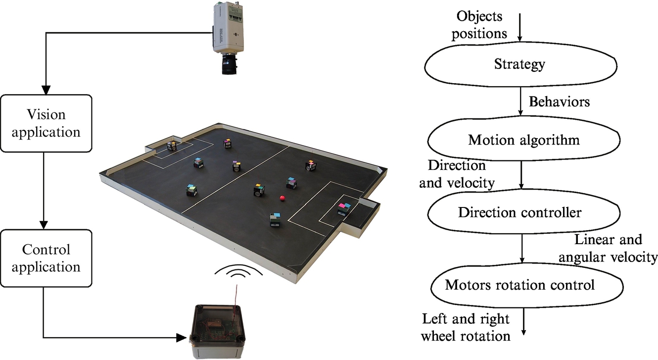
The camera is mounted above the playground and is used to track objects (ball and players) from their color information [4]. Basic operation of the agent program is shown in Fig. 8.19. A personal computer first assigns behavior to each agent. Behavior contains an algorithm for defining the direction and velocity of an agent. The direction controller calculates the desired translational and angular velocity of the robot and sends it as a reference command to the robot via a radio connection. An onboard PID controller achieves desired robot wheel velocities. Note that any other kind of wheeled mobile robot that is capable of sensing its position and position of the ball can be used in this exercise.
The exercise comprises three sections, where in each section a subsystem is developed that is required for implementation of the complete multiagent system. In the first section the desired agents’ simple motion capabilities are programmed to retrieve the ball and kick it in the opponent’s goal, to defend the goal, and to avoid collisions. The second section introduces a behavior-based operation of a single agent. The last section introduces a multiagent system where more agents are playing cooperatively in a team considering a simple game strategy.
8.6.2 Motion Control
The first task requires coding a motion control algorithm in order to approach the ball from the right direction and push it toward the goal. On the other side the goalkeeper should control its motion in front of the goal line to block the goal shuts.
Attacker Motion Control
The basic operation of an attacking robot is to move to the ball and push it toward the goal. Therefore its reference pose contains the reference position, which is the position of the ball (xref, yref), while the reference orientation (φref) is the desired direction of the ball motion after the kick (see Fig. 8.20).

To hit the goal location (xg, yg) the reference orientation is
where ![]() is the four-quadrant version (see Eq. 6.43) of the inverse tangent (in Matlab use atan2 function).
is the four-quadrant version (see Eq. 6.43) of the inverse tangent (in Matlab use atan2 function).
Is the performance of the control algorithm sufficient in cases when the ball (xb, yb) moves? For moving the ball a robot should predict the ball’s future position and intercept it there. A general predicted ball position solution for nonstraight robot motion is difficult to compute analytically. Therefore, suppose the robot can move on a straight line as shown in Fig. 8.21.

From the dot product,

angle α is computed. Then angle β that defines the required relative robot driving direction is expressed using law of sines ![]() and angle γ = π − α − β. Finally from
and angle γ = π − α − β. Finally from ![]() the time needed for the robot to reach the ball reads
the time needed for the robot to reach the ball reads
And the predicted ball or reference position is

Note, however, that this calculated predicted reference position can only be successfully used for controlling robot motion if the robot initially is facing the reference position and the desired kicking direction is close to φ. This, however, is rarely true because the true robot path is usually longer than the direct line supposed in the calculation. The robot initially is not facing the predicted reference position and the final kick direction needs to be toward the goal. If one can approximately estimate the true path length l to reach point xref, yref with orientation φref then the robot speed can be adjusted to reach the predicted ball in time t, as follows ![]() .
.
Straight Accelerated Kick Motion Control
As already mentioned the moving ball can be kicked quite accurately in the goal if the robot’s initial position faces toward the goal xg, yg with accelerated motion. The situation is illustrated in Fig. 8.22.
An unknown reference point can be calculated from current ball position and its known motion:

or from the following robot position,

where t is time when the robot can reach the ball with the requested straight motion and p scalar parameter. Combining Eqs. (8.28), (8.29) results in the following matrix equation:
which is in form Au = b and its solution is u =A−1b. A feasible solution requires 0 < p < 1, meaning that the interception ball point is between the robot and the goal. The reference point then reads
and the required robot acceleration a considering its current velocity v reads

Exercise
Write a motion control algorithm that will kick a moving ball in the goal using straight accelerated motion. If a solution is possible compute the required acceleration using Eq. (8.31). This is computed in each control loop iteration and a new robot translational speed is set to v(k) = v(k − 1) + a(k − 1)Ts, where v(k) is the current velocity and v(k − 1) is the previous velocity. Angular velocity needs to be controlled so that the robot will drive in the desired direction ![]() . Test the algorithm’s performance.
. Test the algorithm’s performance.
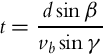
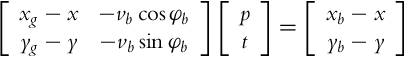
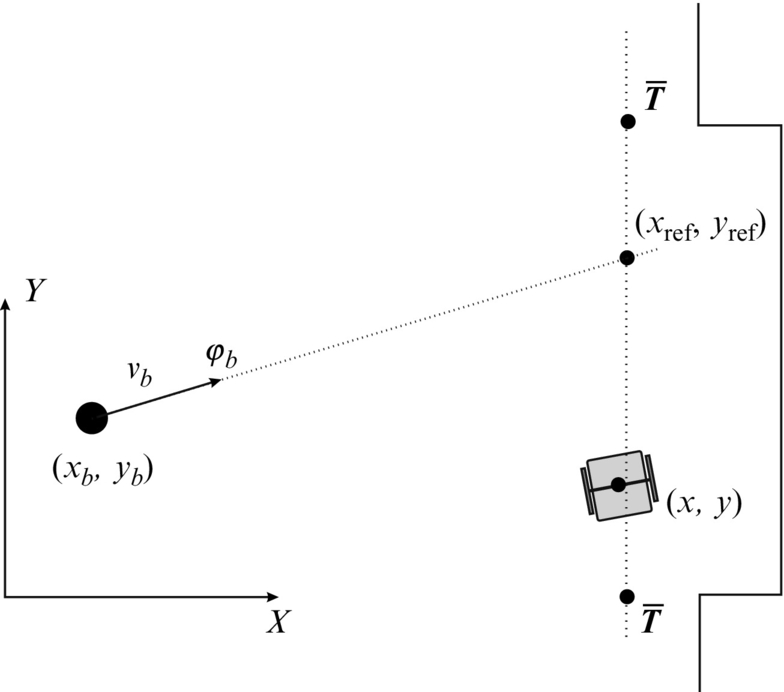
Goalie Motion Control
Goal keeping robot motion control could be as follows. Suppose the robot drives on a goal line between points ![]() and
and ![]() , as shown in Fig. 8.23. Its current reference position xref, yref on the dotted line needs to be calculated according to the ball position xb, yb and its velocity vector vb in direction φb to predictively move to the location where the ball will pass the dotted line. From known data compute the time in which the ball will cross the goal line and the reference position
, as shown in Fig. 8.23. Its current reference position xref, yref on the dotted line needs to be calculated according to the ball position xb, yb and its velocity vector vb in direction φb to predictively move to the location where the ball will pass the dotted line. From known data compute the time in which the ball will cross the goal line and the reference position

where xg is the coordinate of the goal line.
To drive the robot along the goal line a linear trajectory tracking controller described in Section 3.3.5 could be used, where reference velocities (vref, ωref) in the reference position are zero. The control law therefore simplifies to
where gains kx, ky, and kφ can be constants determined by experimenting. Local errors ex, ey, and eφ are calculated using Eq. (3.35) and eφ must be in the range − π < eφ ≤ π.
Exercise
Write a control algorithm that would position the goal keeping robot on the goal line (dotted line in Fig. 8.23) to defend the goal. Test the robot’s performance by pushing the ball from different locations toward the goal. Observe the controller performance in the case of large tracking errors ![]() ; can this be improved?
; can this be improved?
Obstacle Avoidance
If a playground is surrounded by a fence or there are more players on the playground, then the robot’s motion control algorithm should also consider obstacle avoidance. One way to achieve such behavior is the use of the potential field method, similarly as introduced in Section 4.2.4.
8.6.3 Behavior-Based Agent Operation
Suppose you have three robots playing in the same team. The first robot is the goalkeeper, the second is the attacker, and the third is the midfield player. For each of the players or agents there are different behaviors possible inside their role (e.g., goalkeeper) according to the current situation in the game (their position, position of the ball, or other players). In the current moment each agent needs to decide which behavior it will perform. This behavior selection can be realized by reactive behavior-based architecture, which means that from the currently sensed environment information and internal agent knowledge the most appropriate behavior is selected autonomously. If there are more behaviors possible, then the one with the higher priority is chosen.
For instance the goalkeeper needs to be positioned in the goal area; if this is not the case then it needs to drive in the goal. This goal-arriving behavior can be set as the highest priority. If it is in the goal then it needs to defend the goal. It needs to calculate where the ball would pass the goal line and position itself to this location before the ball arrives. If the ball is not rolling toward the goal it can position itself in the center of the goal line.
The attacker agent can use basic motion control without ball prediction if its velocity is too small to reach the moving ball; otherwise, it can use predictive motion. If the conditions for accelerated straight kick are valid, then it should perform accelerated straight-kick behavior. Additionally it should detect possibility of collision and try to avoid collision. However, in some situations (e.g., when it possessed the ball) it should not try to avoid other players or opponents.
The third player is a midfield player, which means that it should try to place itself at some (predefined) locations on the playground and orient itself toward the opponent goal. It therefore needs to arrive to the defined location, and if it is at the location then it needs to rotate to face toward the goal. This agent currently seems useless if agents’ roles are static, but if they can change dynamically (agent can decide during the game to be attacker, goalie or midplayer) it becomes important, as seen in the next section.
8.6.4 Multiagent Game Strategy
Running all previously defined agents together should result in an autonomous soccer-like game. Here, make the agents choose autonomously which role (goalie, attacker, or midplayer) they will play. For each role define some numerical criteria such as the following examples: distance to the ball and distance to the goal. Each agent needs to evaluate those criteria and choose the role that they can currently perform with the highest success of all other agents. First you can evaluate agents for the goalkeeper role (e.g., which agent is closest to the goal) and the most successful agent becomes the goalkeeper. The goalkeeper is the role with the highest priority because it is assigned first.
The remaining two agents should verify which one can be the best attacker (e.g., which is closest to the ball). And the last agent is the midplayer. The agent that is currently the midplayer can take the role of attacker if the condition for accelerated straight kick becomes valid and the current attacker is not successful (e.g., not close to the ball). To negotiate which agent occupies a certain role the agents need to communicate their numerical criteria to others and then decide. Role assignment can also be done globally.
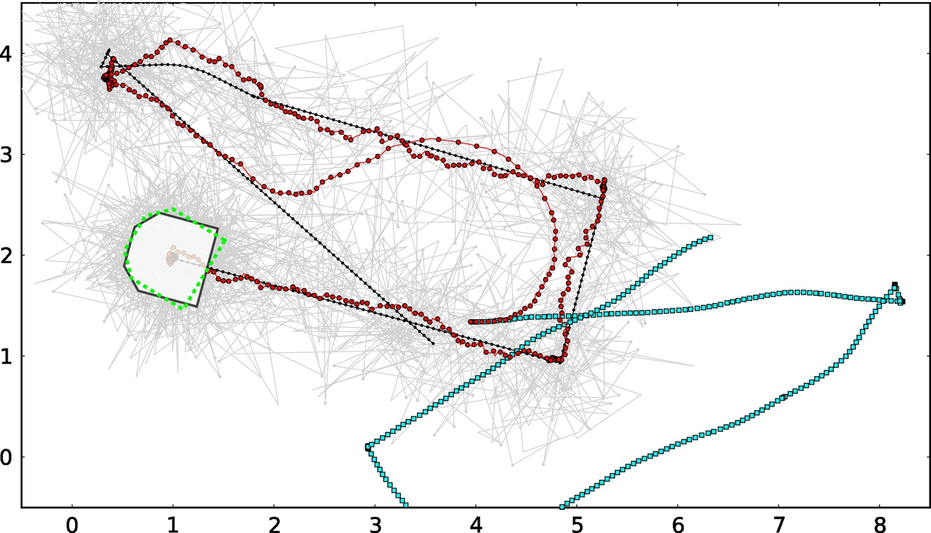
An example of dynamic role assignment during a robot soccer game in [5] is shown in Figs. 8.24 and 8.25. Here, five robots are playing against five opponent robots and the game strategy consists of 11 behaviors, where some of them are very similar to those presented in this exercise.

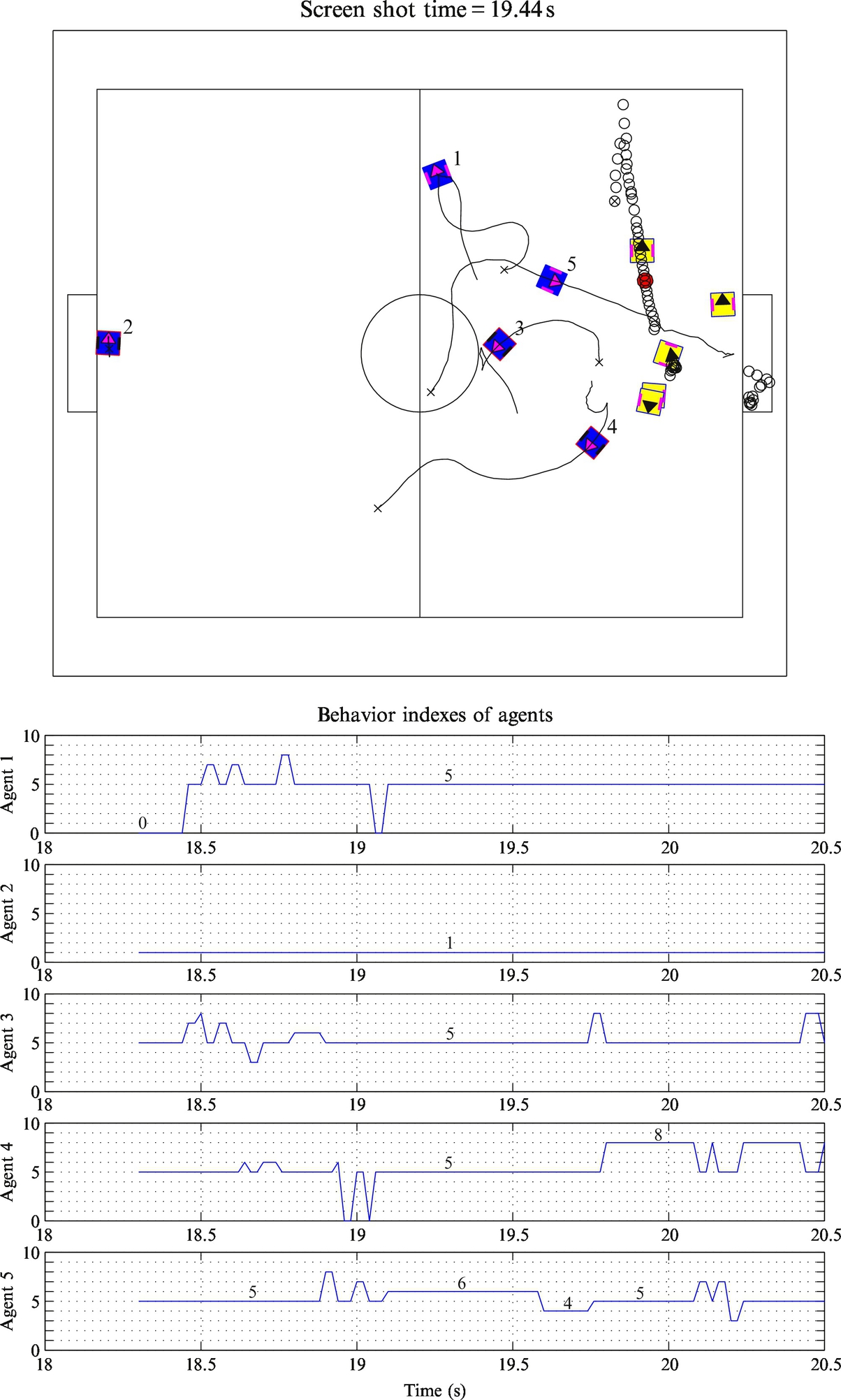
In Fig. 8.24, a long breakthrough of agent 1 is shown. It starts approaching the ball by playing attacker behavior (behavior index 0) and then continuing with approaching to the future interception point of the ball (behavior index 8) in a predictive manner. Finally, agent 1 switches to guider behavior (index 4) and scores a goal. It should be mentioned that opponent players’ positions drawn in Fig. 8.24 correspond to a screen shot time at 12.08 s. The opponent player that seems to block agent 1 and the ball direction has therefore moved away, leaving agent 1 a free pass. From the behavior index plot for the first agent, a sudden jump of behavior index from 4 (ball guider) to 3 (predictive attacker) and then back again can be observed. This happens because the ball moved some distance away from agent 1 when pushing it.
A nice assist of agent 3, which rebounds the ball from the boundary by playing behavior 0, can be seen in Fig. 8.25. After the rebound, the straight ball motion is intercepted by agent 5 playing behavior 6, and the action is finished by behavior 4.
8.7 Image-Based Control of a Mobile Robot
8.7.1 Introduction
Usage of machine vision in control of mobile robots is an emerging field of research and development. A camera is an attractive sensor for use in mobile systems due to its nice properties: noninvasive sensor, a lot of data, relatively small, and a lightweight and affordable sensor. Contemporary capabilities of computer processors enable real-time implementation of computationally intensive image processing algorithms, even on battery-powered embedded systems. However, image processing is considered a difficult problem, due to various reasons: the image is formed as a projection of 3D space, various image distortions and abbreviations, illumination changes, occlusions, and other issues. The required information for control is normally not easy to extract from the huge amount of data the image provides, especially if real-time performance is required.
In this laboratory practice an approach of visual control of a wheeled mobile robot equipped with a camera to a desired location is presented.
8.7.2 Experimental Setup
Usage of a two-wheeled mobile robot with differential drive is assumed. On-board of the mobile robot a front-facing camera is mounted (Fig. 8.26); this is known as eye-in-hand configuration. The considered control algorithms will require in-image tracking of at least four coplanar points. To somewhat simplify image processing some color markers or special patterns can be introduced into the environment; later some more advanced machine vision approaches can be used in order to track some features already present in the environment. The considered configuration is depicted in Fig. 8.26. The pose of the camera C on the mobile robot R is given with rotation matrix ![]() and translation vector
and translation vector ![]() . The desired mobile robot pose is given with respect to the pose of the world frame W, that is, with rotation matrix
. The desired mobile robot pose is given with respect to the pose of the world frame W, that is, with rotation matrix ![]() and translation vector
and translation vector ![]() .
.

8.7.3 Position-Based Visual Servoing
To implement visual control some image processing is required in order to determine control error. There are two basic approaches: the control error can be defined in the 3D frame—this is known as position-based visual servoing (PBVS)—or the control error is determined directly as a 2D error in the image; this is known as image-based visual servoing (IBVS). In this case a PBVS control scheme will be considered. A pinhole camera model (5.48) will be used. Visual servoing normally requires camera calibration, where radial and tangential lens distortion need to be eliminated.
Once the camera is calibrated an appropriate image feature tracking algorithm needs to be implemented. Without loss of generality assume that the camera is observing four corners of a square, which is placed on the ground in the world frame, where the corners of the square are color coded in colors that are unique in the observed environment. Under controlled illumination conditions color patches can be obtained with simple image processing (see Section 5.3.4). It is assumed that the tracked features are always in front of the camera image plane and always visible, that is, in the camera field of view.
Assume that the positions of the four corners of the square, which are placed in the ground plane, in the world frame W are known: ![]() , i = 1, 2, 3, 4. The control goal is to drive the wheeled mobile robot to the origin of the world frame, that is, align the robot frame R with the world frame W. Since the points pW, i, i = 1, 2, 3, 4, in the world frame are constrained to a plane and images of these points are also on a plane, the transformation between the world and image (picture) point can be described by homography (5.56), denoted as
, i = 1, 2, 3, 4. The control goal is to drive the wheeled mobile robot to the origin of the world frame, that is, align the robot frame R with the world frame W. Since the points pW, i, i = 1, 2, 3, 4, in the world frame are constrained to a plane and images of these points are also on a plane, the transformation between the world and image (picture) point can be described by homography (5.56), denoted as ![]() . A point in the image can be transformed to the plane with the origin in the robot frame R. This transformation can be described by homography
. A point in the image can be transformed to the plane with the origin in the robot frame R. This transformation can be described by homography ![]() .
.
Once the positions of the tracked points in the image frame P are transformed to the robot frame R, the control error between the robot frame R and the world frame W can be determined. Using an appropriate control algorithm that is defined directly in the robot frame the wheeled mobile robot can be driven to the goal pose. During execution of the visual control algorithm some image features may leave the camera field of view, and the visual control would fail. Therefore, the feature square should be positioned in an appropriate position in the world plane that prevents this situation. A more appropriate solution would be to design the control algorithm in a way that prevents this situation.
Notice that the tracked features normally cannot be positioned near the origin of the world frame (reference pose), since the camera normally cannot observe the features that are below the mobile robot.
8.7.4 Image-Based Visual Servoing
In this section the same control problem as in previous section will be solved in the IBVS control scheme. Let us initially assume that the camera is mounted on the wheeled mobile robot in a way that the origin of the robot frame R is in front of the image plane, although it may not be visible in the image due to limited field of view.
In this case also the transformation between the image plane P and robot plane R again needs to be determined. This could be made in the same way as already suggested in the previous section. However, here an alternative approach will be considered. The wheeled mobile robot can be positioned into the origin of the world frame W in a way that the robot frame R is aligned with the world frame W. Given known positions of the feature points in the world frame {pW, i}i=1, 2, 3, 4 and measured positions of their projections in the image frame {pP, i}i=1, 2, 3, 4, the homography matrix ![]() can be estimated using the least-squares method based on point correspondences.
can be estimated using the least-squares method based on point correspondences.
Exercise
Estimate homography ![]() using the least-squares method based on point correspondences between world and image points.
using the least-squares method based on point correspondences between world and image points.
Once the homography ![]() is known, the origin of the world frame can be moved around to define the desired reference pose. Square pattern feature points can then be transformed into the image plane to obtain the desired location of the feature points in the image. Comparing current locations of the tracked points with the desired points in the image can be used in order to define control error and design a control algorithm.
is known, the origin of the world frame can be moved around to define the desired reference pose. Square pattern feature points can then be transformed into the image plane to obtain the desired location of the feature points in the image. Comparing current locations of the tracked points with the desired points in the image can be used in order to define control error and design a control algorithm.
Notice that the desired positions of the image features can also be determined without the knowledge of homography ![]() . This can be achieved if the wheeled mobile robot is positioned to the desired pose, and image locations of the tracked features are captured. This approach is sometimes referred to as teach-by-showing.
. This can be achieved if the wheeled mobile robot is positioned to the desired pose, and image locations of the tracked features are captured. This approach is sometimes referred to as teach-by-showing.
8.7.5 Natural Image Features
The control algorithms designed in the previous sections required that a special marker was introduced into the environment. However, some features that are inherently present in the environment can also be used in order to implement visual control. This enables more useful application, since no special preparation of the environment is required. If the ground is flat and contains enough visual cues that can be robustly detected with some machine vision algorithm, the similar control approaches as designed in the previous sections can be used, except that a different feature tracking algorithm is used. Implementations of various feature tracking algorithms can be found in the open source computer vision library OpenCV [6].
8.8 Particle-Filter-Based Localization Using an Array of Ultrasonic Distance Sensors
8.8.1 Introduction
This exercise deals with localization of differentially driven wheeled robots equipped with three ultrasonic distance sensors. An environment where the robot moves is known and described by the sequence of straight line segments. Localization is performed using a particle filter that fuses odometry information and measured sensor information to obtain robot location in the map.
An example of such a robot build from the Lego Mindstorm EV3 kit is shown in Fig. 8.27. This figure also contains a view of the robot environment. Any other robot with distance sensors can also be used in this exercise or if preferred the whole exercise can be done using simulation. Read Section 6.5.3 to get better insight to the localization using a particle filter. This exercise is an upgrade of Example 6.24, which can be used and modified for the purpose of this exercise.

In the following, basic steps that will guide you to the final solution are outlined: prediction of particles’ location using odometry, measurement model for estimation of simulated particle measurement, and correction of particle filter by particle restamping based on their success (importance).
8.8.2 Predicting Particles’ Locations From Known Robot Motion
A particle filter consists of a prediction and correction part. First we will implement a basic framework of the particle filter and implement prediction of the particles’ locations.
Robot pose estimation using odometry needs to be implemented to predict each particle’s future location based on known motion commands sent to the true robot. Suppose motion commands sent to the robot in current time instant k are vk and ωk. With this command all particles are moved from their current pose ![]() to the new predicted pose
to the new predicted pose ![]() , where i is the index of ith particle. The predicted particle pose considering sifting of the time instant
, where i is the index of ith particle. The predicted particle pose considering sifting of the time instant ![]() and sampling time Ts reads
and sampling time Ts reads
8.8.3 Sensor Model for Particle Measurement Prediction
The robot in Fig. 8.27 has three sensors that measure distances to obstacles in three defined directions according to the local robot frame. Each particle presents a hypothesis of the robot position and therefore needs to calculate its measurement. Those measurements are needed to evaluate which particle is the most important (its pose is most likely to be the robot pose). This evaluation is based on comparison of robot and particle measurements.
To calculate simulated particle measurements the environment is first described by straight line segments where each jth segment can be defined by two neighboring points xj−1, yj−1 and xj, yj (see Fig. 8.28) as follows:
where A = yj − yj−1, B = −xj + xj−1 and C = −xj−1A − yj−1B. The distance sensor measurement direction is described by the equation
where ![]() ,
, ![]() , Cs = − xAs − yBs where x, y are robot center coordinates and α is a sensor measurement angle obtained by summing the robot (or particle) orientation and relative sensor angle (αr which in Fig. 8.28 can be 0 degree, 90 degree, or − 90 degree) according to the robot (α = φ + αr). If the straight lines (8.32), (8.33) are not parallel (det = AsA − ABs≠0) then they intersect in
, Cs = − xAs − yBs where x, y are robot center coordinates and α is a sensor measurement angle obtained by summing the robot (or particle) orientation and relative sensor angle (αr which in Fig. 8.28 can be 0 degree, 90 degree, or − 90 degree) according to the robot (α = φ + αr). If the straight lines (8.32), (8.33) are not parallel (det = AsA − ABs≠0) then they intersect in

and measured distance of the simulated sensor (between the robot position and the intersection point) is
This computed distance of course makes sense only if the object is in front of the distance sensor and not behind and if the intersection point is in between the straight line segment, which can be checked by the condition

To obtain the final simulated sensor distance all line segments of the environment need to be checked and minimal distance to one of the lines needs to be found.
8.8.4 Correction Step of Particle Filter and Robot Pose Estimate
The first step in the correction part of the particle filter is estimation of the particles’ simulated measurements. For each particle position and orientation in the simulated environment its measurements are calculated using a derived sensor model. Those measurements are used to evaluate particles by comparing them to the true robot measurement.
8.9 Path Planning of a Mobile Robot in a Known Environment
In order to find the optimum path between the obstacles from the current mobile robot pose to the desired goal pose a path planning problem needs to be solved. This is an optimization problem that requires a known map of the environment and definition of optimality criterion. We can look for the shortest path, the quickest path, or the path that satisfies some other optimality criterion. This exercise covers the A* algorithm that is one of the commonly used approaches of solving the path planning problem.
8.9.1 Experimental Setup
This exercise does not require any special hardware. The task is to develop an algorithm that can find an optimum path between an arbitrary start and goal location given a map of the environment. The map can be represented in various ways, but in this experimental setup we will assume that the map is available as an occupancy grid. An example of an occupancy grid is represented as a grayscale image in Fig. 8.29A, which consists of 170 × 100 square pixels (width of each pixel corresponds to 10 cm in the real world). The particular occupancy map has the following color coding: white pixels (value 255)—free space, light-gray pixels (value 223)—unknown space, dark-gray pixels (value 159)—border. The map shown Fig. 8.29A has been acquired automatically with an SLAM approach. However, the map can also be drawn manually in any image manipulation software or even hard-coded into a file.
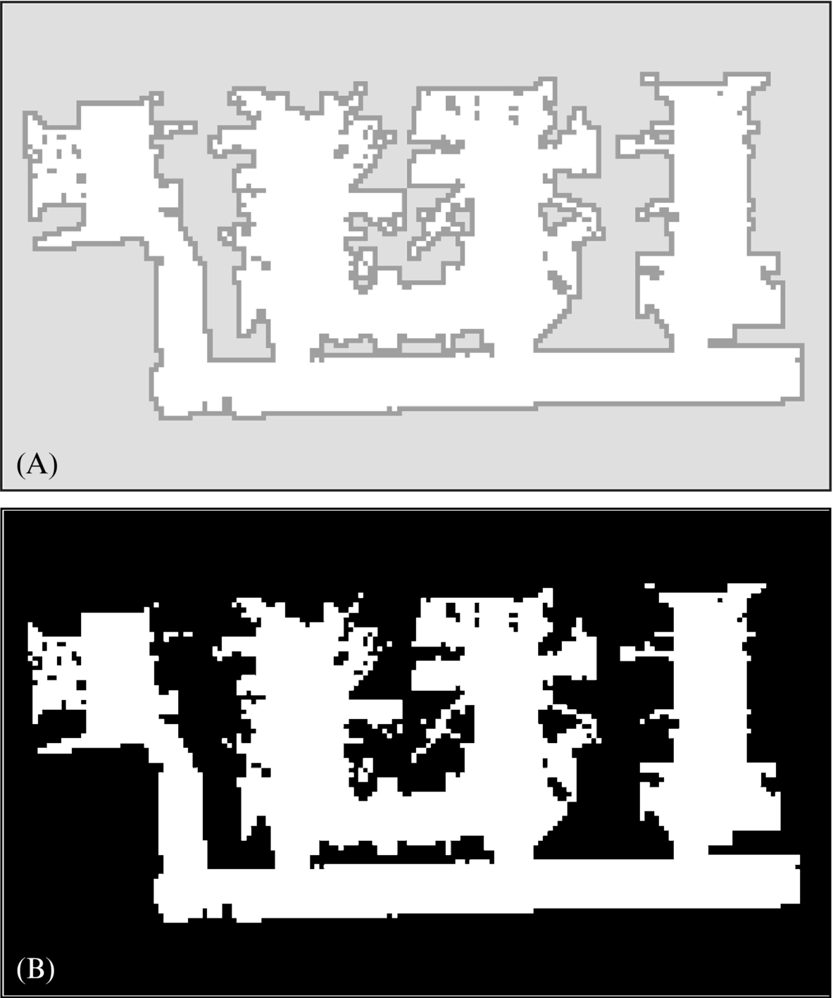
For the purpose of path planning we will assume that the robot can only move inside a free space. In this case it is therefore adequate to represent an occupancy grid with only two color levels, as a binary image where white pixels correspond to free space and black pixels correspond to a nontraversable space. Thresholding the occupancy map in Fig. 8.29A with the threshold level 160 results in a binary image (map) shown in Fig. 8.29B.
8.9.2 A* Path Searching Algorithm
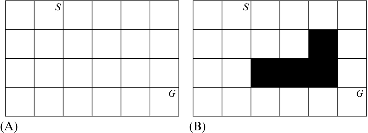
For the purpose of algorithm development we will use a simple and small map of the environment, with and without obstacles. Examples of small maps that are appropriate for algorithm development are shown in Fig. 8.30; the dimensions of the map grids are 6 × 4 cells. The map in Fig. 8.30A is without obstacles and the map in Fig. 8.30B contains a single L-shaped obstacle. The start and end locations are marked with letters S and G, respectively.
In the A* algorithm a direct distance from any cell in the map to the goal needs to be determined (neglecting any obstacles on the way). For this purpose different distance measures can be used, for example, Manhattan or Euclidean distance.
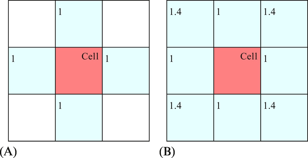
The A* search algorithm begins exploring the map in the start cell (node) and expands the search looking at the connected neighbors. In the A* algorithm immediate neighbors of the currently active cell need to be determined. In a regular grid map a four-cell or eight-cell neighborhood around the cell is normally used (Fig. 8.31). For each cell in the neighborhood a transition cost Δg from the center cell needs to be defined. In Fig. 8.31 Euclidean distance is used, although some other measure could also be used (e.g., cost d for any vertical and horizontal move and cost 3 for any diagonal move).
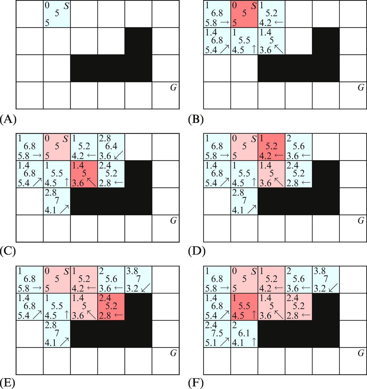
In an A* search algorithm an open and closed list of cells are used. The open list contains all the cells that need to be searched, and the closed list contains the cells that have already been processed. All the cells in the open list are ordered according to cost-of-the-whole-path, which is a sum of the cost-to-here and cost-to-goal (also known as heuristic). Initially only the start cell is in the open list. Until there are cells in the open list and the goal cell is not reached, the cell with the lowest cost-of-the-whole-path is set as the active cell. The active cell is removed from the open list and added to the closed list. The cost-to-here, cost-to-goal, and cost-of-the-whole-path are calculated and an index of source cell is remembered for each neighbor around the active cell that is not an obstacle. If the neighbor is not already in the open or closed list, it is added to the open list. If the cell is already in the closed or open list and the new cost-to-here is lower, the cell is moved to the open list, and all costs and also the index of the source cell are updated. A more detailed description of the algorithm can be found in Section 4.4.5.
If the goal cell has been reached, the optimum path from the start to the goal can be obtained by tracking back the source cells from the goal until the start cell is reached.
Exercise
Implement an algorithm for obtaining the path if the goal cell has been reached. Write a function that enables visualization of the path. Validate the algorithm with the visualization of all the steps shown in Figs. 8.32 and 8.33.


8.9.3 Optimum Path in the Map of the Environment
Although some automatic mapping approach can be used, in this case we will manually draw a map of the environment.
Fig. 8.34 shows an optimum path between the start and goal obtained by the A* path searching algorithm, where the searched cells (pixels) are also marked. The basic path searching algorithm requires some modifications in order to obtain the feasible path that the robot can follow. As it can be noted from Fig. 8.34, the optimum path is close to the obstacle boundaries. Since the robot dimensions are nonzero, the obtained path may not be feasible for the robot to follow.
The problem of nonzero mobile robot dimensions can be solved in various ways. Assume that the robot can fit inside a circle with the radius r = 40 cm around the rotation center of the robot. In this case the map of the environment can be modified in a way that the free space in the vicinity of the obstacles, at distances below r, is considered as occupied space. The path searching can then be used without any other modifications, that is, the mobile robot can be assumed to be dimensionless. Fig. 8.35 shows the result of the path searching algorithm with extended obstacle boundaries.
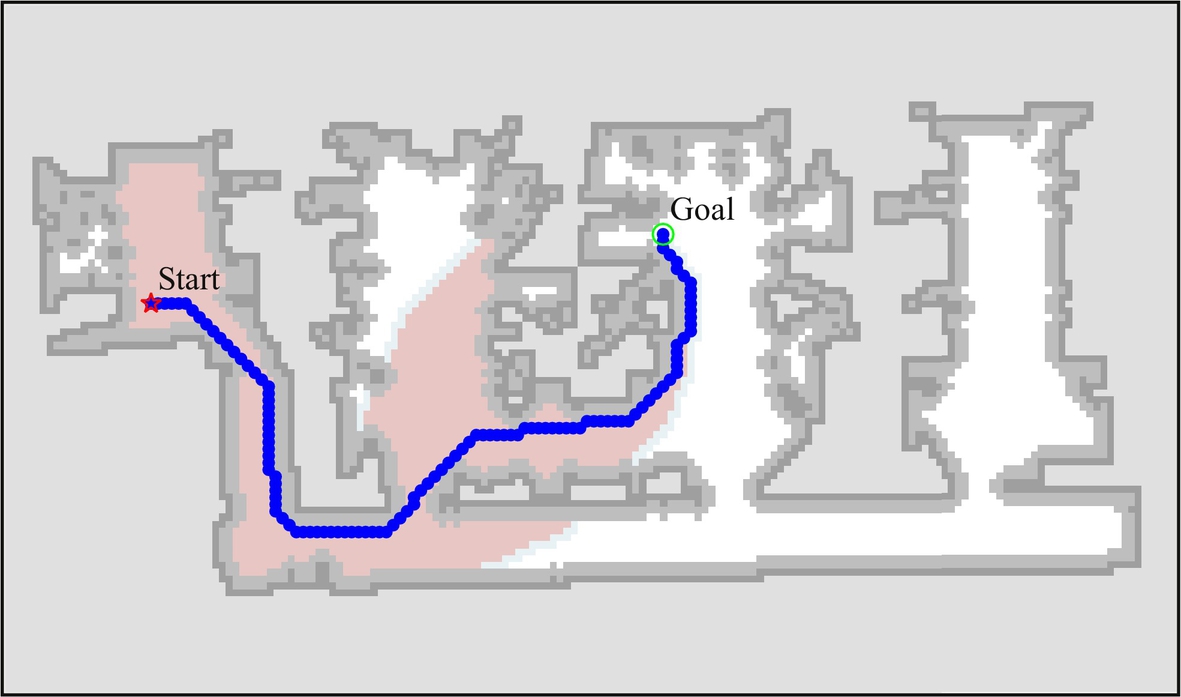
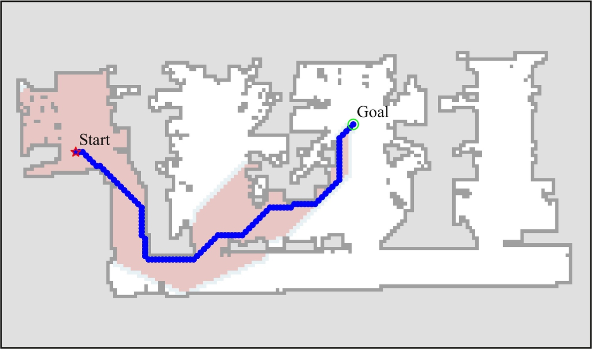
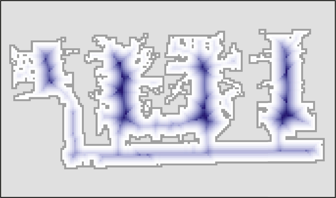
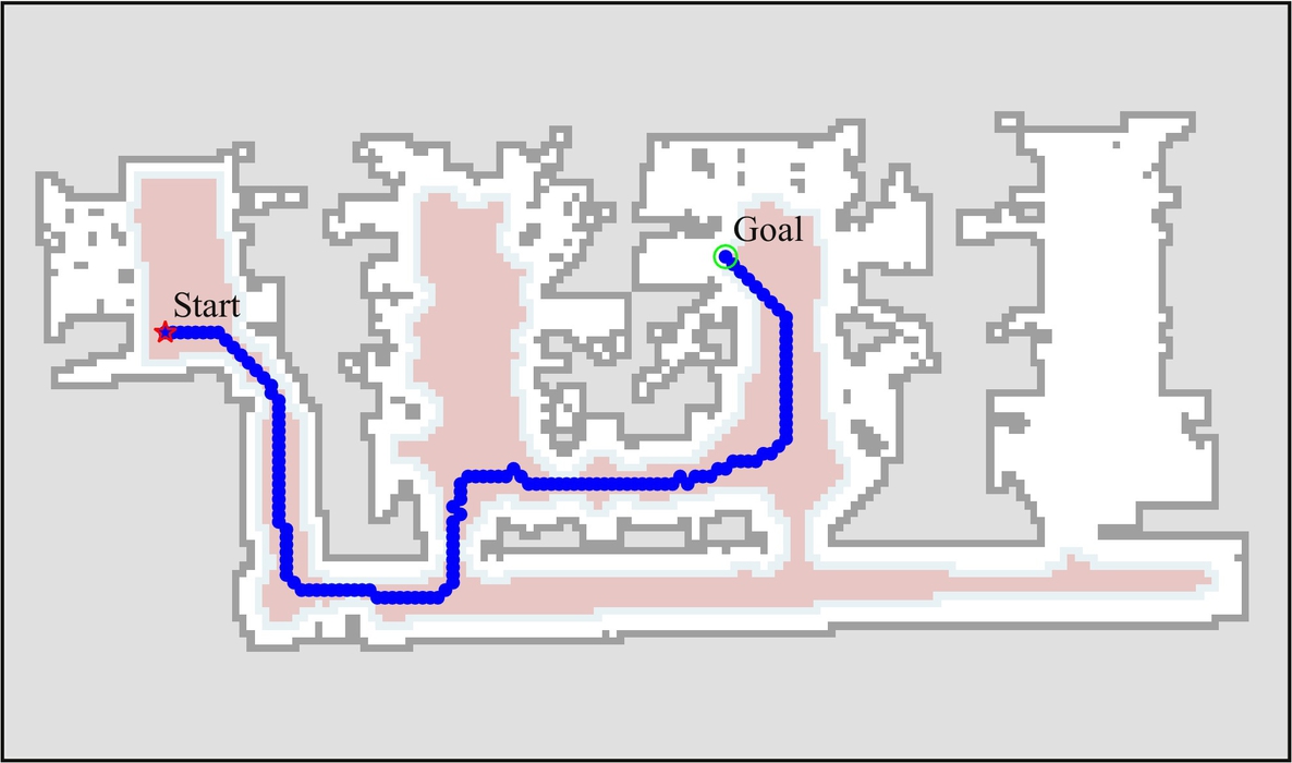
The approach of extending the obstacle boundaries to take the robot dimensions into account may lead to separation of free space into multiple unconnected areas. This may also happen to narrow passages that the mobile robot should be able to pass through but were blocked due to too wide obstacle boundaries, since the obstacles’ boundary extension is normally larger than the robot’s size. An alternative approach is to use distance transform. For every point the free space, a distance to the nearest obstacle is calculated. A visualization of distance transform is shown in Fig. 8.36. The distance inverse can then be added to the cost-to-goal (heuristic). In this way paths that are further away from the obstacles are preferred; therefore, better paths can be obtained that are optimally away from the nearest obstacles. In Fig. 8.37 it can be seen that the obtained path is along the middle of the corridors.
Some additional aspects of the path planning algorithm can be found on a webpage [7], which includes many interactive examples.