There is a mobile robot that drives around on a plane and measures its position with a GPS sensor 10 times in a second (sampling time Ts = 0.1 s). The position measurement is disturbed with zero-mean Gaussian noise with variance 10 m2. The mobile robot drives with the speed of 1 m/s in the x direction and with the speed of 0 m/s in the y direction. The variance of Gaussian noise of the velocity is 0.1 m2/s2. At the beginning of observation, the mobile robot is situated in the origin x = [0, 0]T, but our initial estimate about the mobile robot’s position is xˆ=[3,3]T with initial variance
P0=[100010]
What is the time evolution of the position estimate and the variance of the estimate?
Solution
The solution of the problem can be obtained with the aid of simulation tools provided in Matlab. Let us determine the robot’s movement model where the state estimate represents the robot’s position in a plane xˆk|k−1=[xk,yk]T and input u = [vx, vy]T represents the robot’s speed in x and y directions, respectively. The model for system state prediction is therefore
xˆk|k−1=[1001]xˆk−1|k−1+[Ts00Ts]u
The position measurement model of a GPS sensor is
zˆk=[1001]xˆk|k−1
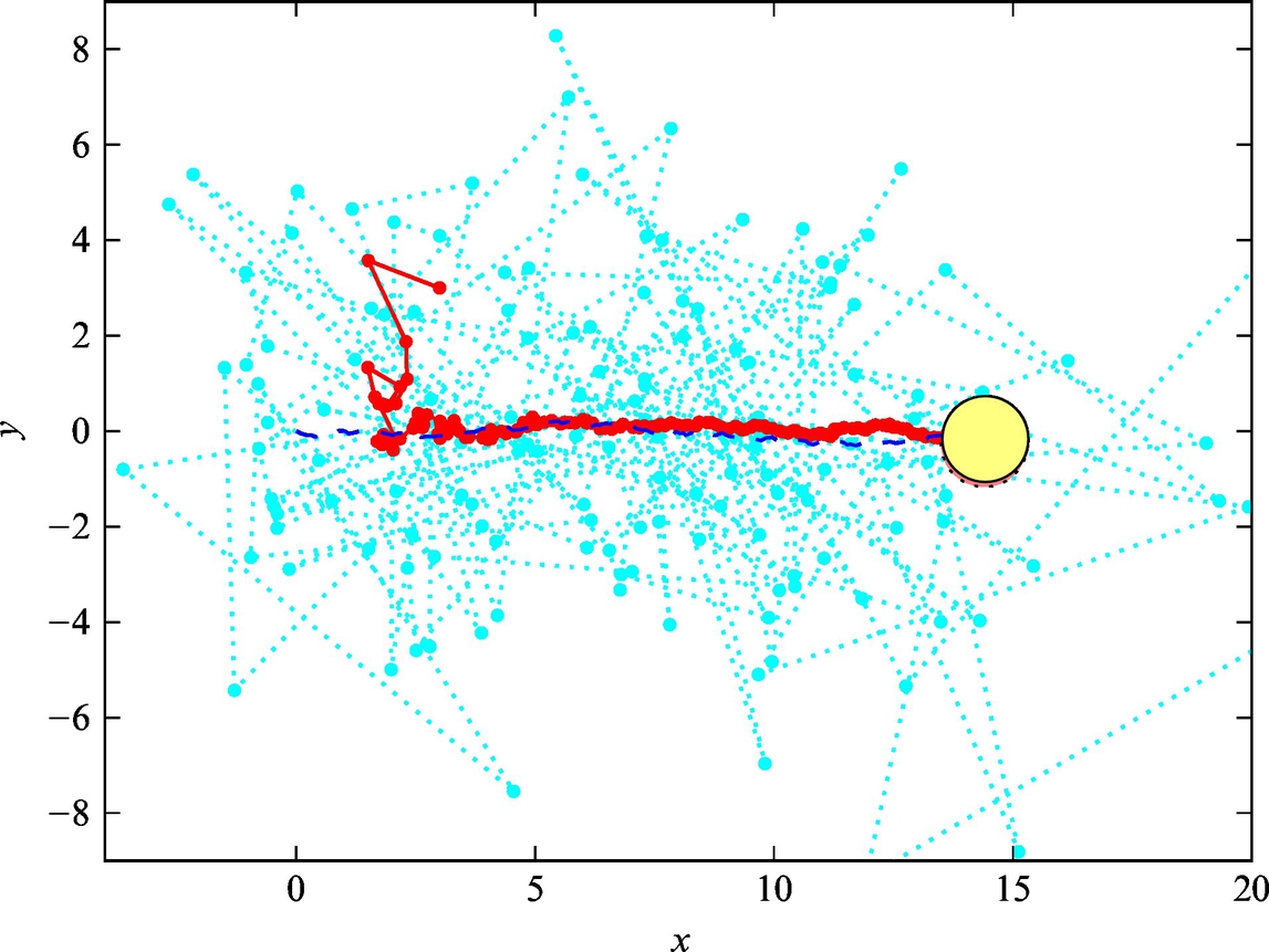
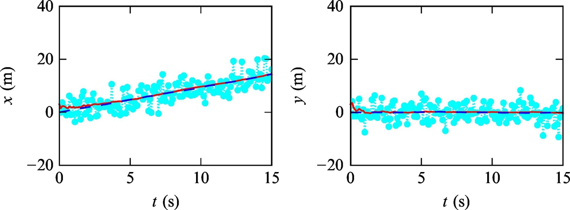
Listing 6.10 provides an implementation of the solution in Matlab. The simulation results are shown graphically in Figs. 6.20–6.22. The simulation results confirm that the algorithm provides a position estimate that is converging to the true robot position from the false initial estimate. This is expected since the mean of the measurement noise is zero. However, the estimate variance is decreasing with time and falls much below the measurement variance (the internal kinematic model is the trusted mode). The Kalman filter enables optimum fusion of data from different sources (internal kinematic model and external measurement model) if variances of these sources are known. The reader should feel free to experiment with system parameters and observe the estimate variance evolution and convergence rate.
10 P = diag([10 10]) ; % Variance of theInitial state estimate
11 Q = diag([1 1]/10) ; % Noise variance of the movement actuator
12 R = diag([10 10]) ; % Noise vairace of the GPS measurements
13
14 figures _ k f 1 _ i n i t ;
15
16 % Loop
17 N = 150;
18 for k= 1:N
19 u= [ 1 ; 0 ] ; % Movement command
20
21 % Simulation of the true mobile robot position and measurement
22 xTrue= A *xTrue+ B *u+ F*sqrt(Q)*randn(2 , 1) ;
23 zTrue= C *xTrue+ sqrt(R)*randn(2 , 1) ;
24
25 % Position estimate based on known inputs and measurements
26 % %% Prediction
27 xPred= A *x+ B *u ;
28 PPred= A *P* A. ’ + F* Q *F . ’ ;
29
30 % %% Correction
31 K = PPred* C. ’/(C *PPred* C. ’ + R) ;
32 x= xPred+ K*( zTrue − C * xPred ) ;
33 P = PPred − K * C * PPred ;
34
35 figures_kf1_update ;
36 end
Fig. 6.20 True (dashed line) and estimated (solid line) trajectory with measurements (dotted line) from Example 6.19. The final position of the robot is marked with a circle.
Fig. 6.21 True position (dashed line) and position estimate (solid line) of the mobile robot based on measurements (dotted line) from Example 6.19.
Fig. 6.22 Time evolution of mobile robot position variance from Example 6.19.
6.5.2 Extended Kalman Filter
The Kalman filter was developed for linear systems, and it is normally assumed that all disturbances and noises can be described with a zero-mean Gaussian distribution. Noise with a Gaussian distribution is invariant to linear transformations, or in other words, if Gaussian noise is transformed by a linear function, it remains Gaussian noise; it only has different noise parameters that can be calculated explicitly given the known linear function. This is the reason behind the computational efficiency of the Kalman filter. In the case the input Gaussian noise is transformed by a nonlinear function, the output noise is no longer Gaussian, but it can normally still be approximated with a Gaussian noise.
If any of the state transitions or output equations of the system are a nonlinear function, the conventional Kalman filter may no longer produce an optimum state estimate. To overcome the problem of nonlinearities, an extended Kalman filter (EKF) was developed where the system nonlinearities are approximated with local linear models. The local linear model can be obtained from a nonlinear system with the procedure of function linearization (first-order Taylor series expansion) around the current state estimate. In the process of linearization the sensitivity matrices (Jacobian matrices) for current values of estimated states and measurements are obtained. The obtained linear model enables approximation of the noise that is not necessarily Gaussian with a Gaussian noise distribution.
The use of noise linearization in the process of noise modeling enables a computationally efficient implementation of the EKF algorithm. Hence, the EKF algorithm is commonly used in practice. The accuracy of linear approximation depends on the noise variance (big uncertainties or noise amplitudes may lead to poor linear approximation, since the signal may be outside the linear region) and the level of nonlinearity. Due to the error that is caused by linearization the convergence of the filter can worsen or the estimation may not even converge to the true solution.
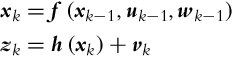
A nonlinear system may be written in a general form:
xkzk=f(xk−1,uk−1,wk−1)=h(xk)+vk
(6.37)
where the noise wk can occur at the system input or influence the states directly.
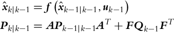
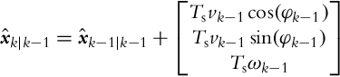
The EKF for a nonlinear system (6.37) has a prediction part:
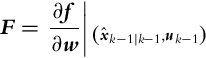
In the prediction part (6.38) the nonlinear state transition system is used for calculation of state prediction estimate. To calculate the noise covariance matrix, the Jacobian matrix A that describes the noise propagation from previous to current states and the Jacobian matrix F that describes the noise propagation from inputs to the states need to be determined from the state model (6.37):
A=∂f∂xˆ∣∣(xˆk−1|k−1,uk−1)
(6.40)
F=∂f∂w∣∣(xˆk−1|k−1,uk−1)
(6.41)
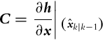
In the correction part (6.39) the measurement estimate is made based on predicted state estimate zˆk=h(xˆk|k−1). The Jacobian matrix C that describes the noise propagation from states to outputs also needs to be determined:
C=∂h∂x∣∣(xˆk|k−1)
(6.42)
The noise covariance matrices are Qk=E{w(k)wT(k)} and Rk=E{v(k)vT(k)}. Among many applications, the EKF has been successfully applied for solving the wheeled mobile robot localization problem [7, 8] and map building [9].
Example 6.20
Awheeled mobile robot with a differential drive moves on a plane. The robot input commands are the translational velocity vk and angular velocity ωk that are both disturbed independently by Gaussian noise with zero mean and variances var{vk}=0.1m2/s2 and var{ωk}=0.1rad2/s2, respectively.
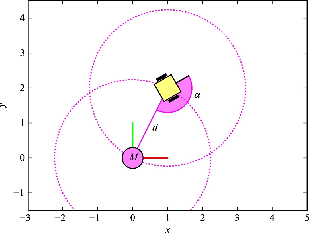
The mobile robot has a sensor that enables measurement of the distance to the marker that is positioned in the origin of the global coordinate frame. The robot is also equipped with a compass that enables measurement of the mobile robot’s orientation (heading). The considered setup is presented in Fig. 6.23. The distance measurement is disturbed by a Gaussian noise with zero mean and variance 0.5 m2, and the angle measurement is also disturbed by Gaussian noise with zero mean and variance 0.3 rad2.
Fig. 6.23 Setup considered in Example 6.20. The mobile robot has a sensor for measuring the distance to marker M (positioned in the origin of the global frame) and a compass to determine the robot orientation in the global frame (heading).
At the beginning of observation the true initial pose of the robot is x0 = [1, 2, π/6]T; however, the initial estimated pose is xˆ0=[3,0,0]T with initial variance:
P0=⎡⎣⎢900090000.6⎤⎦⎥
What is the time evolution of the mobile robot pose estimate (xˆk|k−1=[xk,yk,φk]T) and the variance of the estimation if the command u=[vk,ωk]T=[0.5,0.5]T is sent to the robot in every sampling time step Ts = 0.1 s?
Solution
The solution can be obtained with the aid of simulation tools provided in Matlab. Let us determine the kinematic motion model of the mobile robot. In this case the kinematic model is nonlinear:
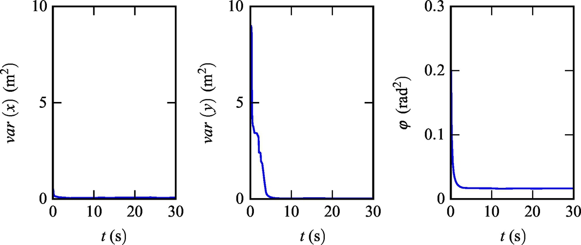
Listing 6.11 provides an implementation of the solution in Matlab. The simulation results are shown in Figs. 6.24–6.28. Simulation results confirm that the algorithm can provide an estimate of the pose that converges to the true pose of the mobile robot although the initial estimate was biased. The innovation terms settle around zero.
29 % %% Prediction (pose and speed estimation based on known inputs)
30 xPred= x+ Ts *[u(1) *cos(x (3) ) ; …
31 u(1) *sin(x (3) ) ; …
32 u(2) ] ;
33 xPred (3) = wrapToPi( xPred (3) ) ;
34
35 % Jacobian matrices
36 A = [1 0 − Ts * u (1) * sin(x (3) ) ; …
37 0 1 Ts*u(1) *cos(x (3) ) ; …
38 0 0 1 ] ;
39 F= [ Ts*cos(x (3) )0; …
40 Ts*sin(x (3) )0; …
41 0 Ts ] ;
42 PPred= A *P* A. ’ + F* Q *F . ’ ;
43
44 % Estimated measurements
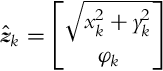
45 z= [sqrt( xPred (1) ˆ2+ xPred (2) ˆ2) ; …
46 xPred (3) ] ;
47
48 % %% Correction
49 d= sqrt( xPred (1) ˆ2+ xPred (2) ˆ2) ;
50 C = [ xPred (1) /d xPred (2) /d0 ; …
51 0 0 1 ] ;
52 K = PPred* C. ’/(C *PPred* C. ’ + R) ;
53 inov= zTrue − z ;
54 inov (2) = wrapToPi( inov (2) ) ;
55 x= xPred+ K *inov ;
56 P = PPred − K * C * PPred ;
57
58 figures_ekf1_update ;
59 end
Fig. 6.24 True (dashed line) and estimated (solid line) trajectory from Example 6.20.
Fig. 6.25 Pose estimate (solid line) and true state (dashed line) of the mobile robot with a nonzero initial estimation error from Example 6.20.
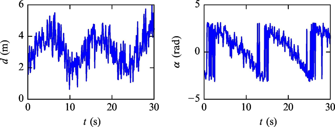
Fig. 6.26 Distance and angle measurements from Example 6.20.
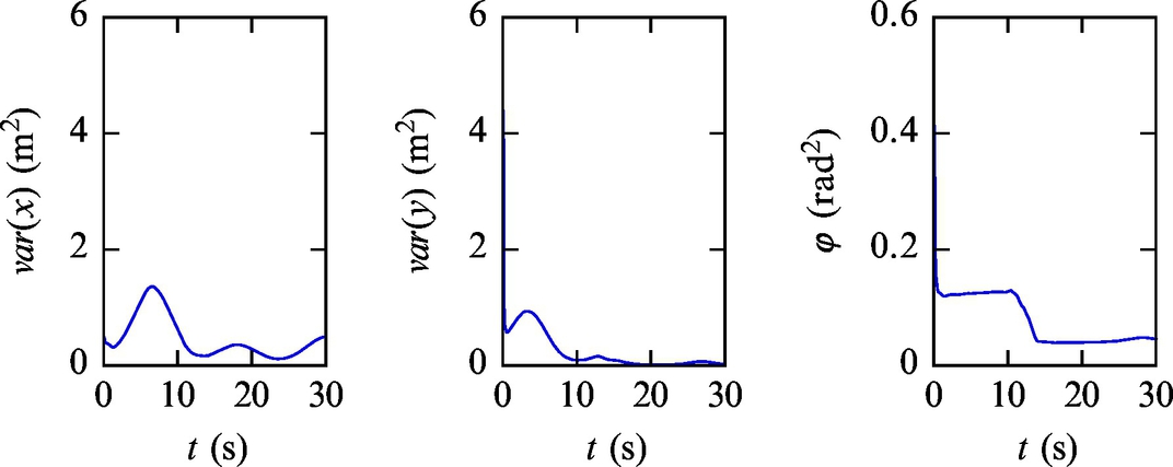
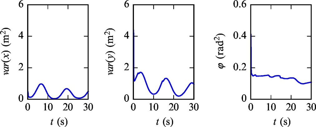
Fig. 6.27 Robot pose estimate variances from Example 6.20.
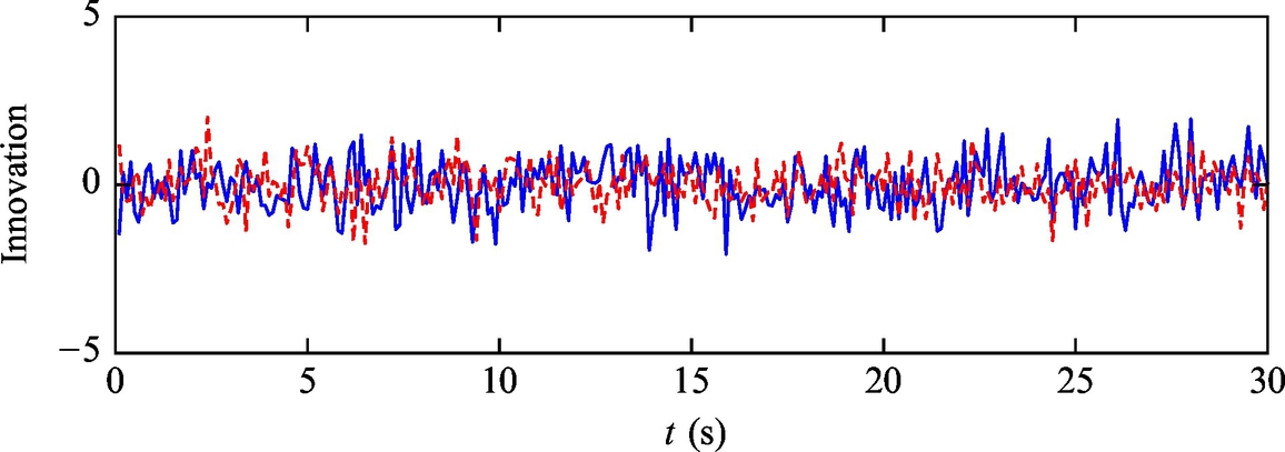
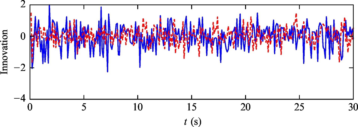
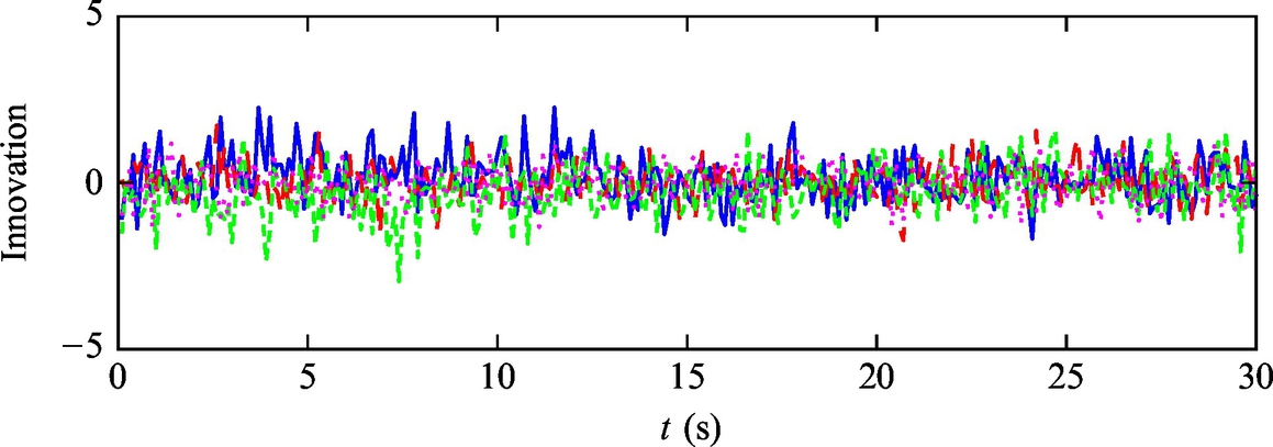
Fig. 6.28 Time evolution of innovation from Example 6.20.
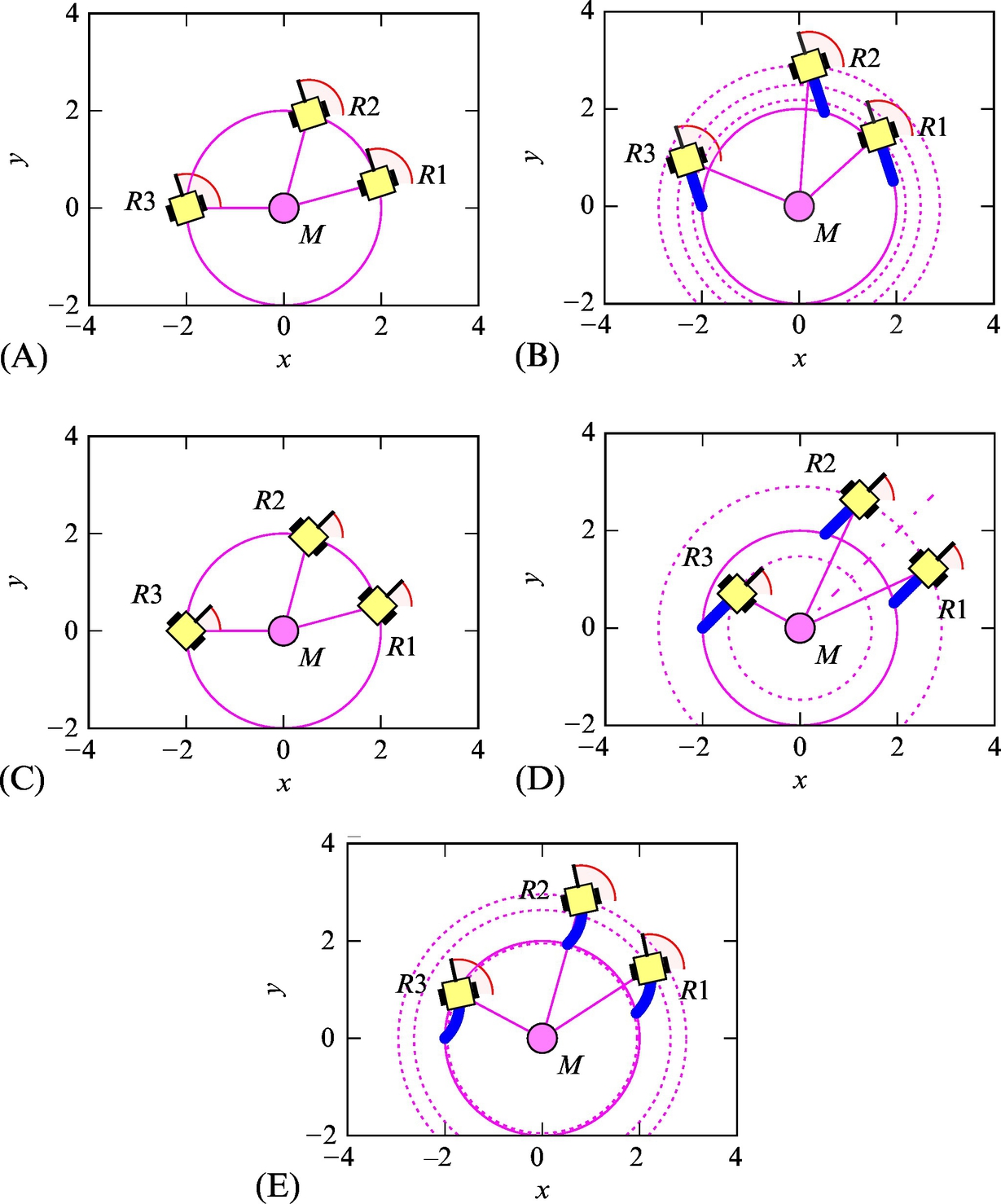
When the states of the system are not measurable directly (as in this example), the question of system state observability arises. Observability analysis approaches can normally provide only sufficient conditions for system observability. However, observability analysis should be performed before designing a state estimation, since it can aid the designer choosing the appropriate set of measurement signals that make the estimation feasible. Although advanced mathematical tools could be used to check system observability, the observability analysis can also be performed with a simple graphical check that is based on the definition of indistinguishable states (see Section 6.3.3). The observability analysis of the system from this example is made in Fig. 6.29. The results in Fig. 6.29 demonstrate that the states of the system are normally distinguishable, except for some special cases (Fig. 6.29D). However, if the system states are observed long enough and mobile robot control inputs are adequately excited, the system is observable.
Fig. 6.29 Observability analysis of the system from Example 6.20. (A) Three particular initial robot poses that all have the same heading and distance from the marker. (B) Updated situation from Fig. (A) after the robots have traveled the same distance in a forward direction. From the measurement point of view, the robot poses are distinguishable. (C) Three particular initial robot poses that all have the same heading and distance from the marker: a special case. (D) Updated situation from Fig. (C) after the robots have traveled the same distance in a forward direction. From the measurement point of view, the robot in pose 1 is indistinguishable from the robot in pose 2, but the robot in pose 3 is distinguishable from the other two poses. (E) Updated situation from Fig. (C) after the robots have traveled the same not-straight path. From the measurement point of view, the robot poses are all distinguishable.
Example 6.21
Let us use the same mobile robot as in Example 6.20, but let us use a slightly different sensor. Assume that the mobile robot has s sensor for measuring the distance and angle to the marker that is in the origin of the global coordinate frame (Fig. 6.30). The angle measurements are in the range α ∈ [−π, π]. The distance measurement is disturbed by a Gaussian noise with zero mean and variance 0.5 m2, and the angle measurement is disturbed by the Gaussian noise with zero mean and variance 0.3 rad2.
Fig. 6.30 Setup considered in Example 6.21. The mobile robot has a sensor for measuring the distance and angle to marker M (positioned in the origin of the global frame).
What is the time evolution of the robot pose estimate (xˆk|k−1=[xk,yk,φk]T) and estimate variance if the input commands u=[vk,ωk]T=[0.5,0.5]T are sent to the robot in every sampling time step Ts = 0.1 s?
Solution
The solution can be obtained with the aid of simulation in Matlab. Let us determine the mobile robot motion model. The kinematic model of the wheeled mobile robot is the same as in Example 6.20:
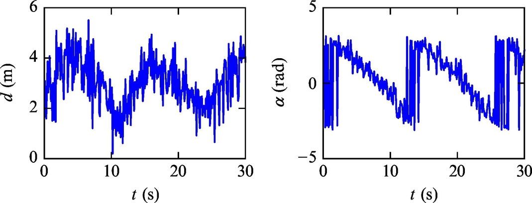
Listing 6.12 provides an implementation of the solution in Matlab. The simulation results in Figs. 6.31–6.35 show that the estimated states converge to the true robot pose. Although this example is similar to Example 6.20, the estimate may not converge to the true robot pose in the presence of only slightly different environmental conditions. The case of convergence to the wrong solution is shown in Figs. 6.36–6.40. Since both sensor outputs (distance and angle) are relative measurements, the estimated states may not converge to the true solution, even though the innovation (difference between measurement and measurement prediction) is in the vicinity of a zero value (Fig. 6.40).
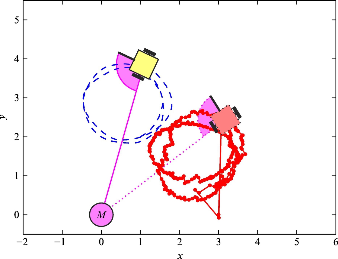
Fig. 6.31 True (dashed line) and estimated (solid line) trajectory from Example 6.21.
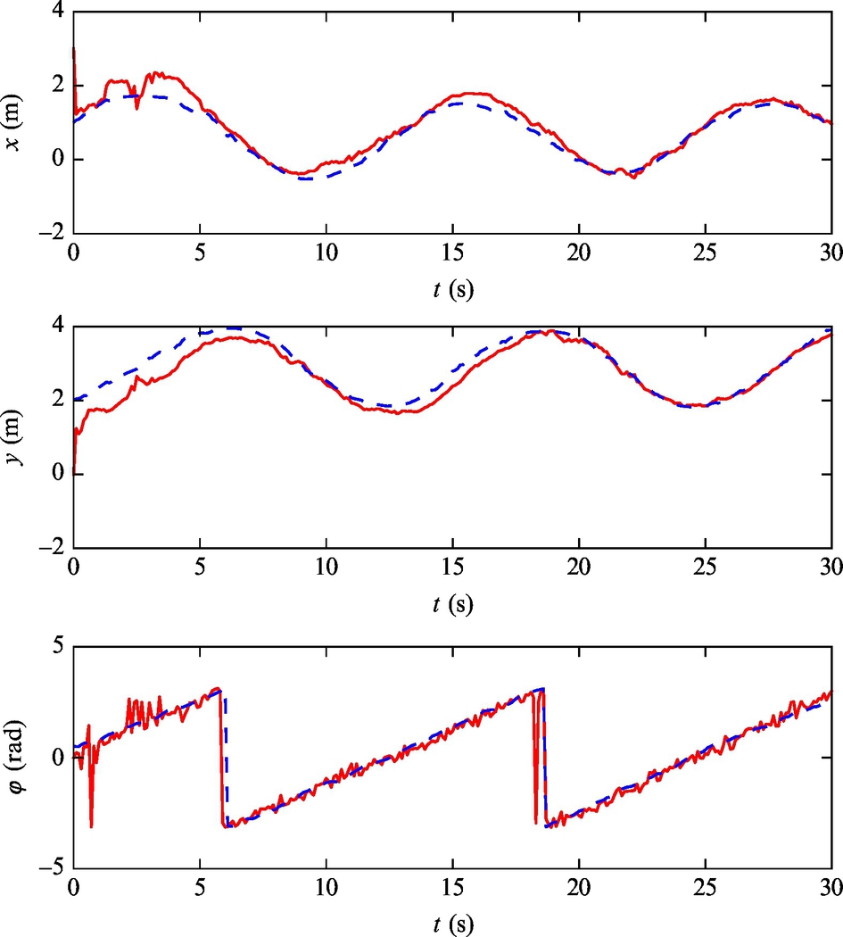
Fig. 6.32 Pose estimate (solid line) and true state (dashed line) of the mobile robot with a nonzero initial estimation error from Example 6.21.
Fig. 6.33 Distance and angle measurements from Example 6.21.
Fig. 6.34 Robot pose estimate variance from Example 6.21.
Fig. 6.35 Time evolution of innovation from Example 6.21.
Fig. 6.36 True (dashed line) and estimated (solid line) trajectory from Example 6.21 (representative case).
Fig. 6.37 Pose estimate (solid line) and true state (dashed line) of the mobile robot with a nonzero initial estimation error from Example 6.21 (representative case).
Fig. 6.38 Distance and angle measurements from Example 6.21 (representative case).
Fig. 6.39 Robot pose estimate variance from Example 6.21 (representative case).
Fig. 6.40 Time evolution of innovation from Example 6.21 (representative case).
8 % Selection of appropriate innovation due to noise and angle wrapping
9 inov (2) = wrapToPi( inov (2) ) ;
10
11 x= xPred+ K *inov ;
12 P = PPred − K * C * PPred ;
13
14 figures_ekf2_update ;
15 end
A graphical check of observability made in Fig. 6.41 can provide additional insight into the reasons for estimation bias. The analyses show that there are states that are clearly indistinguishable from the measurement point of view, regardless of control inputs. Moreover, for every measurement there is an infinite number of states that agree with the measurement.
Fig. 6.41 Observability analysis of the system from Example 6.21. (A) Three particular initial robot poses with same distance from the marker. (B) Updated situation from Fig. (A) after the robots have traveled the same distance in a forward direction. From the measurement point of view, all three robot poses are distinguishable. (C) Three particular initial robot poses that all have the same angle to and distance from the marker: a special case. (D) Updated situation from Fig. (C) after the robots have traveled the same distance in a forward direction. From the measurement point of view, all three robot poses are indistinguishable. (E) Updated situation from Fig. (C) after the robots have traveled the same not-straight path. From the measurement point of view, all three robot poses are indistinguishable.
Therefore, the system is not observable. The estimation bias can be eliminated if multiple markers are observed simultaneously, since this would provide enough information to select the appropriate solution, as it is shown in Example 6.22.
Example 6.22
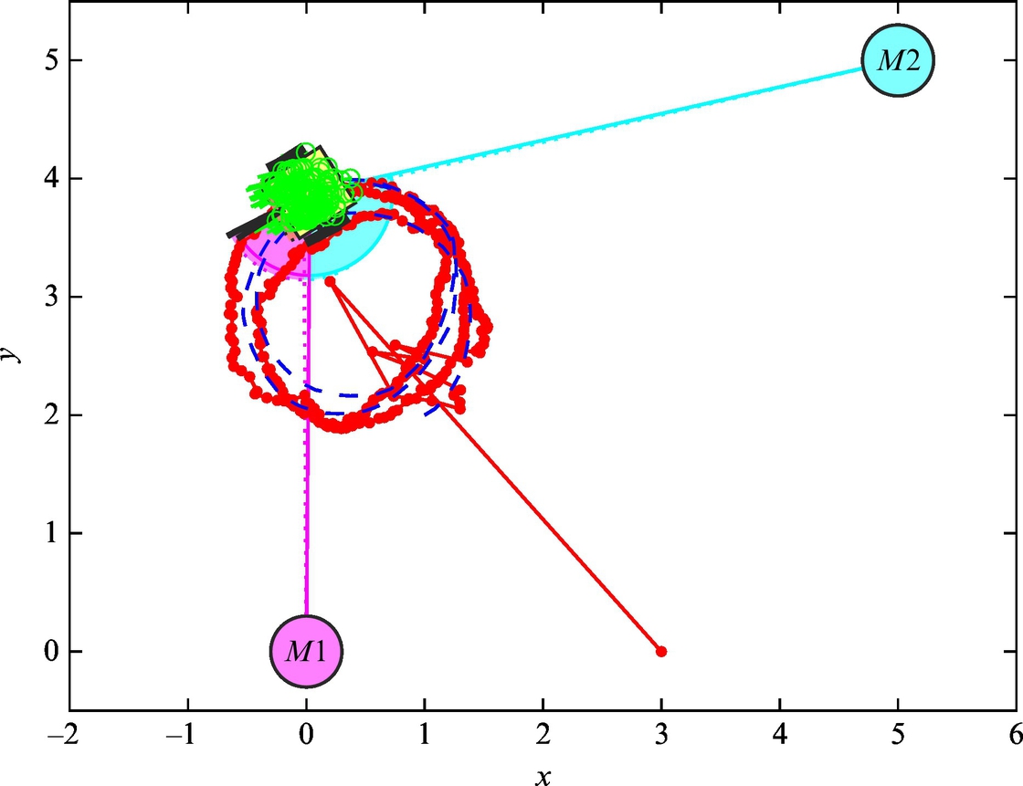
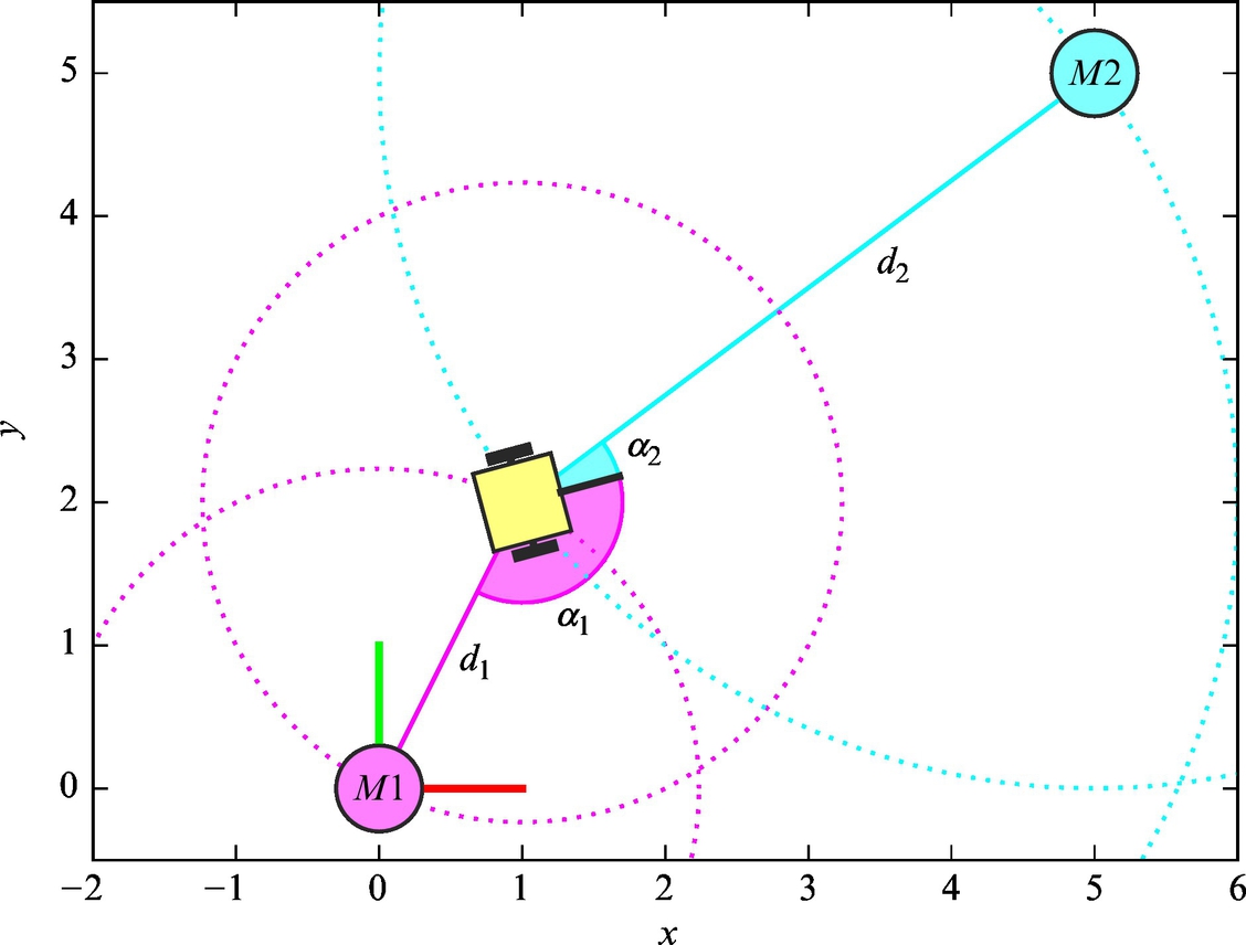
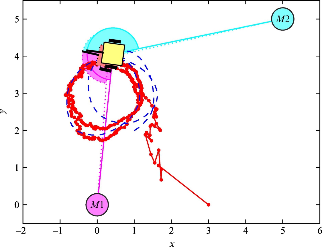
This is an upgraded Example 6.21, in a way that now two spatially separated markers, instead of only one, are observed simultaneously. In this case the sensors measure the distances and angles to two markers (with respect to the mobile robot pose), which are positioned at xM1 = 0, yM1 = 0 and at xM2 = 5, yM2 = 5 in the plane (Fig. 6.42). Otherwise, all the data are identical to Example 6.21.
Fig. 6.42 Setup considered in Example 6.22. The mobile robot has a sensor for measuring the distance and angle to markers M1 and M2.
Solution
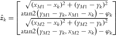
In this case only the correction part of the algorithm needs to be modified. The measurement vector now contains four elements, the distance and angle to the first marker, and also the distance and angle to the second marker:
where d1=(xM1−xk)2+(yM1−yk)2−−−−−−−−−−−−−−−−−−−−−√ and d2=(xM2−xk)2+(yM2−yk)2−−−−−−−−−−−−−−−−−−−−−√. Let us also determine the measurement noise covariance matrix that is
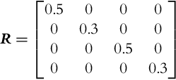
R=⎡⎣⎢⎢⎢⎢0.500000.300000.500000.3⎤⎦⎥⎥⎥⎥
Listing 6.13 provides an implementation of the solution in Matlab. The simulation results are shown in Figs. 6.43–6.47. The obtained results confirm that the estimated states converge to the true robot pose.
Fig. 6.43 True (dashed line) and estimated (solid line) trajectory from Example 6.22.
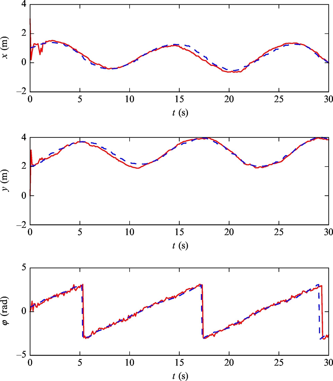
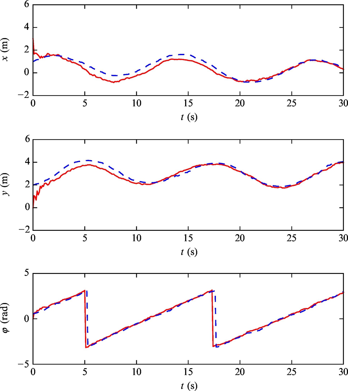
Fig. 6.44 Pose estimate (solid line) and true state (dashed line) of the mobile robot with a nonzero initial estimation error from Example 6.22.
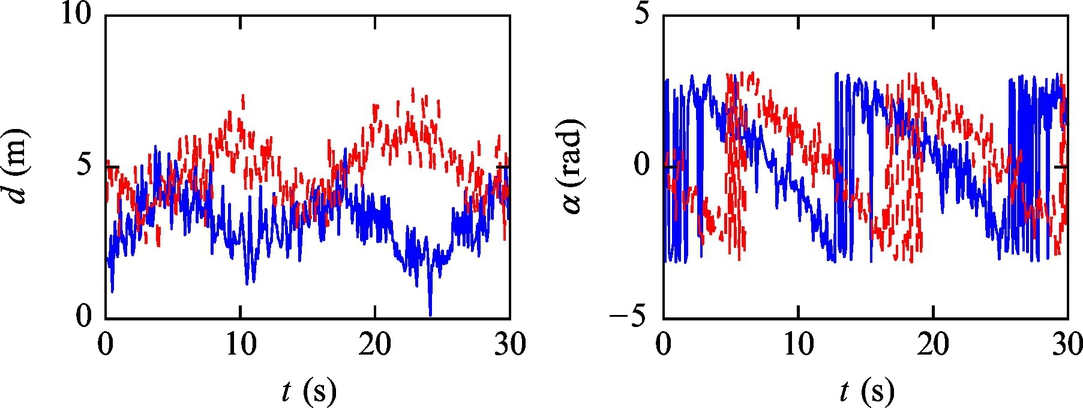
Fig. 6.45 Distance and angle measurements from Example 6.22.
Fig. 6.46 Robot pose estimate variance from Example 6.22.
Fig. 6.47 Time evolution of innovation from Example 6.22.
63 − xPred (2) / d i s t ˆ2 xPred (1) / dist ˆ2−1];
64 C = [ C ; c ] ;
65 end
66
67 % Measurement covariance matrix
68 RR = diag( repmat ( [R(1 ,1) R(2 ,2) ] , 1 ,s i z e ( marker , 1) ) ) ;
69 K = PPred* C. ’/(C *PPred* C. ’ + RR) ;
70
71 inov = zTrue − z ;
72 % Selection of appropriate innovation due to noise and angle wrapping
73 for m = 1: s i z e ( marker , 1)
74 inov (2* m )= wrapToPi( inov (2* m ) ) ;
75 end
76
77 x = xPred+ K*( inov ) ;
78 P = PPred − K * C * PPred ;
79
80 figures_ekf3_update ;
81 end
Again a simple graphical observability check can be performed. In this case one particular situation that has indistinguishable states can again be found, as shown in Fig. 6.48. At first glance the considered states are indistinguishable from the measurement point of view. But since we assume that the measurement data also contains marker IDs, this particular special situation has distinguishable states, and therefore the system is observable.
Fig. 6.48 Observability analysis of the system from Example 6.22. (A) Two particular poses that are symmetrical from the measurement point of view. (B) Updated situation from Fig. (A) after the robots have traveled the same relative path. From the measurement point of view, the both robot poses are distinguishable if measurement data contains IDs of the markers.
6.5.3 Kalman Filter Derivatives
Alongside the Kalman filter for linear systems and the EKF for nonlinear systems [10], many other extensions of the above filters have been proposed. Let us take a look at some of the most common and important approaches.
Unscented Kalman filter [11] is normally used in systems with significant nonlinearities where the EKF may not provide satisfactory results. In this case, the covariance matrices are estimated statistically based on a small subset of points that are transformed over the nonlinear function; the transformed points are used to estimate the mean value and the covariance matrix. These points are known as sigma points that are spread around the estimated value by some algorithm (normally there are 2n + 1 points for n dimensions).
Information filter uses the information matrix and information vector instead of the covariance matrix and state estimate. The information matrix represents the inverse of the covariance matrix, and the information vector is the product of the information matrix and estimated state vector. The information filter is dual to the Kalman filter where the correction step is computationally much simpler to evaluate (no matrix summation). However, the prediction step becomes more computationally demanding.
The Kalman-Bucy filter is a form of the Kalman filter for continuous systems.
6.6 Particle Filter
Up until now the Bayesian filter was considered to be normally used for discrete state-space systems with a finite number of values that the state-space variables can take. If we want to apply the Bayesian filter for continuous variables, these variables can be quantified to a finite number of values. This kind of Bayesian filter implementation for continuous state variables is commonly known as the histogram filter.
For continuous state-space variables an explicit solution of the Bayesian filter (6.29) would need to be determined:
where we took into account the complete state assumption and that the system is a Markov process (see Section 6.2). The current state probability distribution (6.44) is needed in calculation of the most probable state estimate (mathematical expectation):
E{xˆk|k}=∫xk|k⋅p(xk|z1:k,u0:k−1)dxk|k
An explicit solution of Eq. (6.44) is possible only for a limited class of problems where Gaussian noise distribution and system linearity are assumed; the result is a Kalman filter. In the case of nonlinear systems, the system nonlinearity (in the motion model, actuator model, and/or sensor model) can be linearized, and this leads to the EKF.
A particle filter is a more general approach where noise distribution need not be Gaussian and the system may be nonlinear. The basic idea behind the particle filter is that the a posteriori state estimate probability distribution (6.29), after the measurement was made, is approximated with a set of N particles. Every particle in the set presents the value of the estimated state xik that is randomly sampled from the probability distribution (Monte Carlo simulation approach). Every particle represents a hypothesis about the system state. The representation of the probability distribution with a set of randomly generated particles is a nonparametric description of probability distribution, which is therefore not limited to only Gaussian distributions. The description of probability distribution with particles enables modeling of nonlinear transformation of noise (actuator and/or sensor model). The particles can therefore be used to describe the noise distributions that are transformed over nonlinear functions from inputs or outputs to the system states.
Algorithm 5 presents the basic implementation of the particle filter.
Algorithm 5
Particle Filter Algorithm. The Particle_filter Function Is Called in Every Time Step With Current Values of Inputs and Measurement and the Previous State Estimate
functionParticle_filter(xˆk−1|k−1, uk−1, zk)
Initialization:
ifk > 0 then
Initialize a set of N particles xik based on a random sampling of the probability distribution p(x0).
endif
Prediction:
Transform every particle xˆik−1|k−1 based on the known movement model and known input uk−1, to which add a randomly generated value based on the noise properties that are part of the movement model. The movement model is given with p(xk|xk−1, uk−1). The obtained prediction is given as a set of particles xˆik|k−1.
Correction:
For every particle xˆik|k−1estimate measurement output that would be measured if the system state would correspond to the particle state.
Based on the measurement made and comparison against estimated measurements with particles, evaluate the particle importance.
This is followed by importance sampling, a sampling approach based on the particle importance with random selection of the particles in a way that the particle selection probability is proportional to the particle importance (i.e., p(zk|xˆik|k−1)). More important particles should therefore be selected more times, and less important particles fewer times.
Filtered state estimatexˆk|k can be selected as the average value of all the particles.
endfunction
In the initial step of the particle filter an initial population of the particles needs to be selected, xˆi0 for i ∈ 1, …, N, which is distributed based on the belief (probability distribution) p(x0) of the system states at the beginning of observation. In the case the initial state is not known a uniform distribution should be used; therefore, the particles should be spread uniformly over the entire state-space.
In the prediction part a new state for each particle is evaluated based on the known system input. To the state estimate of every particle a randomly generated noise is added, which is expected at the system input. In this way state predictions for every particle are obtained, xˆik|k−1. The added noise ensures that the particles are scattered, since this enables estimation of true value in the presence of different disturbances.
In the correction part of particle filter the importance of the particles is evaluated, in a way that the difference between the obtained measurement zk and all the estimated particle measurements (zˆik) is calculated from estimated particle states. The difference between the measurement and estimated measurement is commonly known as innovation or measurement residual, and it can be evaluated for every particle as
innovik=zk−zˆik
which is low for most probable particles.
Based on measurement residual the importance of every particle, that is, the probability p(zk|xˆik|k−1) can be determined, which represents the weight wik for particle i. The weight can be determined with Gaussian probability distribution as
wik=det(2πR)−12e−12(innovik)TR−1(innovik)
where R is the measurement covariance matrix.
A very important step in the particle filter is importance sampling based on the weights wik. The set of N particles is randomly sampled in a way that the probability of selection a particular particle from a set is proportional of the particle weight wik. Therefore, the particles with larger value of the weight should be selected more times than the particles with lower value of the weight; the particles with the smallest value of the weight should not even be selected. The approach of generating a new set of particles can be achieved in various ways, one of the possible approaches is given below:
•The particle weights wik are normed with the sum of all the weights ∑Ni=1wik; in this way the new weights wnik=wik∑Ni=1wik are obtained.
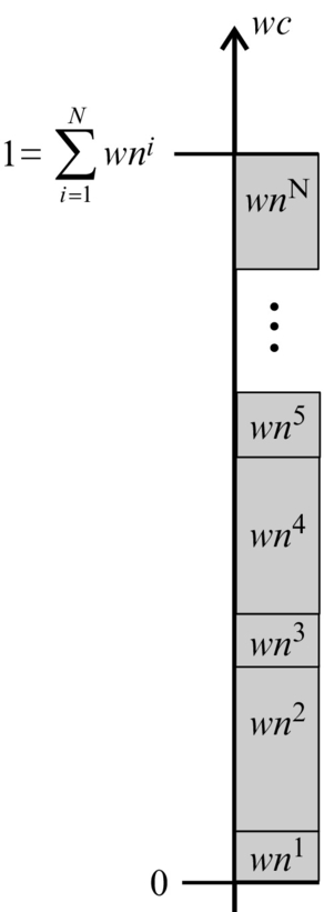
•The cumulative sum of the normed weights is calculated in order to obtain the cumulative weights wcik=∑ij=1wnik, as shown in Fig. 6.49.
Fig. 6.49 Importance sampling in the correction part of the particle filter. The particle weights are arranged in a sequence one after another and then normed in a way that the sum of all the particles is one. More probable particles take more space on the unity interval, and vice-versa. The new population of particles is determined in a way that N numbers from the unity interval are selected randomly (with uniform distribution), and the particles that correspond to these numbers are selected.
•N numbers between 0 and 1 are selected randomly (from a uniform and 1 are selected randomly (from a uniform distribution) and then it is determined to which weights these random numbers correspond. The comparison between the cumulative weights wcik and the randomly generated numbers is therefore made. As seen from Fig. 6.49, the particles with larger weights are more probable to be selected (the weights in Fig. 6.49 occupy more space).
•The selected particles are used in the correction part to determine the a posteriori state estimate xˆk|k=∑Ni=1wikxˆik|k−1.
In the case the system is not moving (the current state is equal to the previous state) it is recommended that the importance sampling is not made, but the previous particles are selected as the current ones and only the weights are modified, as shown in [12].
The application of particle filter is shown in Example 6.23.
Example 6.23
Use a particle filter for estimation of the most likely state in Example 6.22. In the implementation of particle filter use N = 300 particles. All the other data are the same as in Example 6.22.
Solution
Listing 6.14 provides an implementation of the solution in Matlab. The simulation results are shown in Figs. 6.50 and 6.51.
Fig. 6.50 True (dashed line), estimated (solid line) trajectory, and generated particles in the final step of simulation from Example 6.23.
Fig. 6.51 Pose estimate (solid line) and true state (dashed line) of the mobile robot with a nonzero initial estimation error from Example 6.23.
9 iNextGeneration= round( iNextGeneration_float+ 0.5) ; % Round the indices
10 end
In Example 6.23 the distances and angles to the markers are measured, so the angle wrapping must be taken into account. The example of localization where only distances to the markers are measured in order to estimate the mobile robot pose is shown in Example 6.24.
Example 6.24
Use a particle filter for estimation of the most likely state in Example 6.23, but consider only measurement of the distance to the markers. In the implementation of the particle filter use N = 500 particles. All the other data are the same as in Example 6.23.
Solution
Listing 6.16 provides an implementation of the solution in Matlab. The simulation results are shown in Figs. 6.52 and 6.53, where it is clear that the estimated value converges to the true value, as in Example 6.23.
Fig. 6.52 True (dashed line), estimated (solid line) trajectory, and generated particles in the final step of simulation from Example 6.24.
Fig. 6.53 Pose estimate (solid line) and true state (dashed line) of the mobile robot with a nonzero initial estimation error from Example 6.24.
35 iNextGeneration= obtainNextGenerationOfParticles ( W , nParticles ) ;
36 xP= xP ( : , iNextGeneration ) ;
37
38 % The new state estimatei s the average of all thep a r t i c l e s
39 x= mean(xP, 2) ;
40 x (3) = wrapToPi(x (3) ) ;
41 % For robot orientation use the mostl i k e l y p a r t i c l e instead of the
42 % average angle of all thep a r t i c l e s .
43 [ gg , ggi ] = max ( W ) ;
44 x (3) = xP(3 , ggi ) ;
45
46 figures_pf2_update ;
47 end
A particle filter is an implementation of the Bayesian filter for continuous systems (continuous state space); it enables description of nonlinear systems and can take into account arbitrary distribution of noise. Applicability of the particle filter is computationally intensive for high-dimensional systems, since many particles are required to achieve filter to converge. The number of required particles increases with space dimensionality.
The particle filter is robust and is able to solve the problem of global localization and the problem of robot kidnapping. In the problem of global localization the initial pose (the value of the states) is not known. Therefore, the mobile robot can be anywhere in the space. The kidnapping problem occurs when the mobile robot is moved (kidnapped) to an arbitrary new location. Robust localization algorithms must be able to solve these problems.


 are obtained.