Motion Modeling for Mobile Robots
Abstract
This chapter deals with motion modeling of wheeled mobile robots. It starts by introducing kinematic modeling of well-known mobile platforms such as differential drive, bicycle drive, Ackermann drive, and omnidirectional drives. Forward and inverse kinematics are presented, which can be applied in locomotion strategy design or in the localization process. It then describes kinematic motion constraints that originate from the robot structure and its kinematics. Holonomic and nonholonomic constraints are modeled and vector fields analysis using Lie brackets is performed to analyze the system’s constraints and its controllability. At the end, wheeled mobile robots are modeled as dynamic systems using Lagrange formulation where physical properties such as mass, inertia, and force are used. Clear examples of kinematic and dynamic models, constraints analysis, parallel parking maneuver, and the like are presented.
Keywords
Kinematic model; Instantaneous center of rotation; Locomotion; Kinematic constraints; Controllability; Dynamic model; Odometry
2.1 Introduction
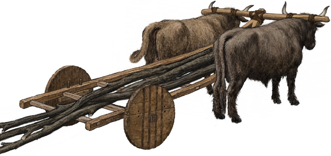
Humans took advantage of wheel drive for thousands of years, and the underlying structure of a prehistoric two-wheeled cart (Fig. 2.1) can be found in modern cars and wheeled robots. This chapter deals with motion modeling of different wheeled mobile systems. The resulting model can be used for various purposes. In this book it will be mainly used for designing locomotion strategies of the system. Locomotion is the process of moving an autonomous system from one place to another.
Motion models can describe robot kinematics, and we are interested in mathematics of robot motion without considering its causes, such as forces or torques. Kinematic model describes geometric relationships that are present in the system. It describes the relationship between input (control) parameters and behavior of a system given by state-space representation. A kinematic model describes system velocities and is presented by a set of differential first-order equations.
Dynamic models describe a system motion when forces are applied to the system. This models include physics of motion where forces, energies, system mass, inertia, and velocity parameters are used. Descriptions of dynamic models are given by differential equations of the second order.
In wheeled mobile robotics, usually kinematic models are sufficient to design locomotion strategies, while for the other systems such as robots in space, air, or walking robots, dynamic modeling is also needed.
2.2 Kinematics of Wheeled Mobile Robots
Several types of kinematic models exist:
• Internal kinematics explains the relation between system internal variables (e.g., wheel rotation and robot motion).
• External kinematics describes robot position and orientation according to some reference coordinate frame.
• Direct kinematics and inverse kinematics. A direct kinematics describes robot states as a function of its inputs (wheel speeds, joints motion, wheel steering, etc.). From inverse kinematics one can design a motion planning, which means that the robot inputs can be calculated for a desired robot state sequence.
• Motion constraints appear when a system has less input variables than degrees of freedom (DOFs). Holonomic constraints prohibit certain robot poses while a nonholonomic constraint prohibits certain robot velocities (the robot can drive only in the direction of the wheels’ rotation).
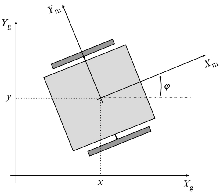
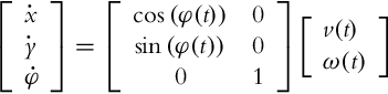
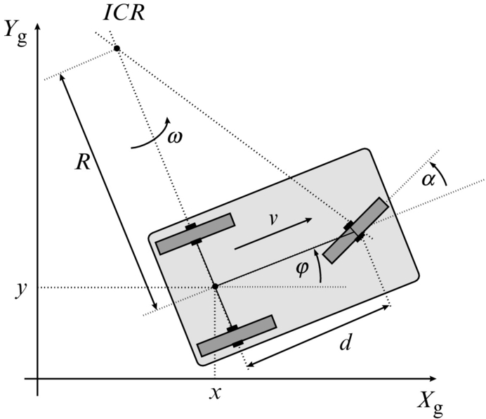
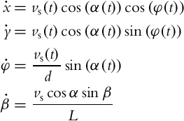
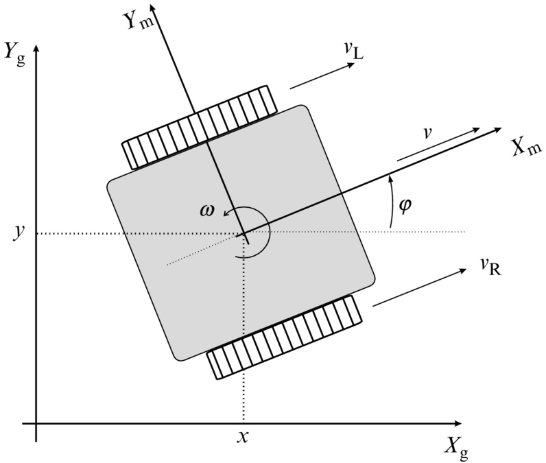
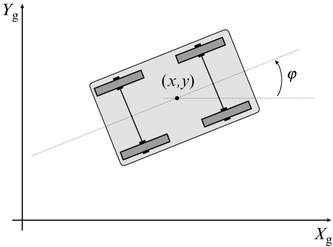
In the following, some examples of internal kinematics for wheeled mobile robots (WMR) will be given. The robot pose in a plane is defined by its state vector
in a global coordinate frame (Xg, Yg), as illustrated in Fig. 2.2. A moving frame (Xm, Ym) is attached to the robot. The relation between the global and moving frame (external kinematics) is defined by the translation vector [x, y]T and rotation matrix:

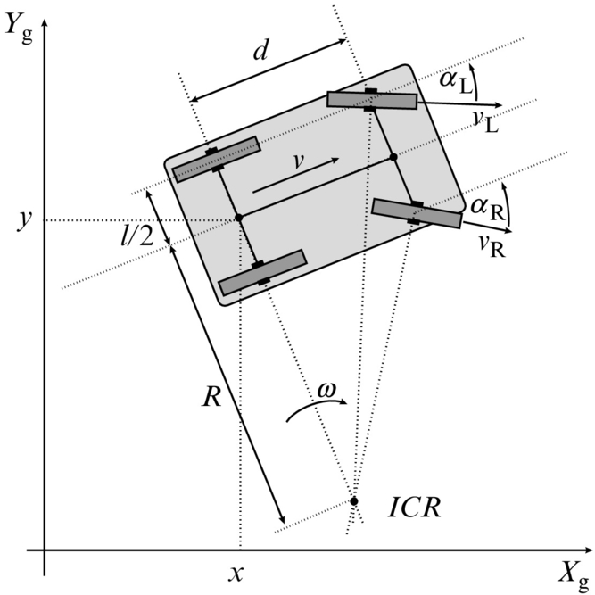
WMR moves on the ground using wheels that rotate on the ground due to the friction contact between wheels and the ground. At moderate WMR speeds an idealized rolling wheel model is usually used where the wheel can move by rotation only and no slip in the driving and lateral direction is considered. Each wheel in WMR can freely rotate around its own axis; therefore, there exists a common point that lies in the intersection of all wheel axes. This point is called instantaneous center of rotation (ICR) or instantaneous center of curvature and defines a point around which all the wheels follow their circular motion with the same angular velocity ω according to ICR. See Refs. [1–3] for further information.
2.2.1 Differential Drive
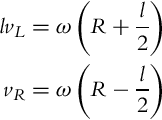
Differential drive is a very simple driving mechanism that is quite often used in practice, especially for smaller mobile robots. Robots with this drive usually have one or more castor wheels to support the vehicle and prevent tilting. Both main wheels are placed on a common axis. The velocity of each wheel is controlled by a separate motor. According to Fig. 2.3 the input (control) variables are the velocity of the right wheel vR(t) and the velocity of the left wheel vL(t).

The meanings of other variables in Fig. 2.3 are as follows: r is the wheel radius; L is the distance between the wheels and R(t) is the instantaneous radius of the vehicle driving trajectory (the distance between the vehicle center (middle point between the wheels) and ICR point). In each instance of time both wheels have the same angular velocity ω(t) around the ICR,
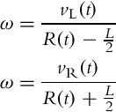
from where ω(t) and R(t) are expressed as follows:
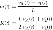
Tangential vehicle velocity is then calculated as

Wheel tangential velocities are vL(t) = rωL(t) and vR(t) = rωR(t), where ωL(t) and ωR(t) are left and right angular velocities of the wheels around their axes, respectively. Considering the above relations the internal robot kinematics (in local coordinates) can be expressed as

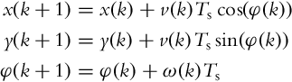
Robot external kinematics (in global coordinates) is given by

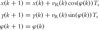
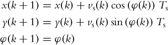
where v(t) and ω(t) are the control variables. Model (2.2) can be written in discrete form (2.3) using Euler integration and evaluated at discrete time instants t = kTs, k = 0, 1, 2, … where Ts is the following sampling interval:
Forward and Inverse Kinematics
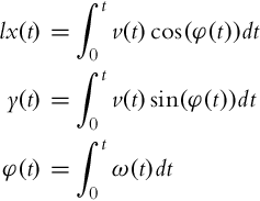
A robot pose at some time t is obtained by integration of the kinematic model, which is known as odometry or dead reckoning. Determination of the robot pose for given control variables is called direct (also forward) kinematics:

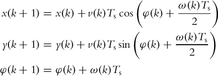
If constant velocities v and ω are assumed during the sample time the integration of Eq. (2.4) can be done numerically using the Euler method. The direct kinematics is then given by
If trapezoidal numerical integration is used a better approximation is obtained as follows:
If exact integration is applied the direct kinematics is
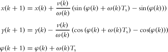
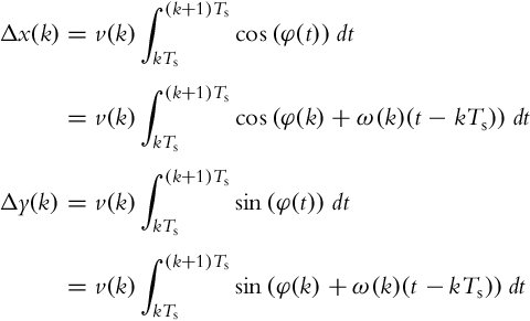
where integration in Eq. (2.7) is done inside the sampling time interval where constant velocities v and ω are assumed to obtain increments:
The development of the inverse kinematics is a more challenging task than the above cases of direct kinematics. We use inverse kinematics to determine control variables to drive the robot to the desired robot pose or path trajectory. Robots are usually subjected to nonholonomic constraints (Section 2.3), which means that not all driving directions are possible. There are also many possible solutions to arrive to the desired pose.
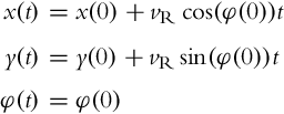
One simple solution to the inverse kinematics problem would be if we allow a differential robot to drive only forward (vR(t) = vL(t) = vR⟹ω(t) = 0, v(t) = vR) or only rotate at the spot (![]() , v(t) = 0) at constant speeds. For rotation motion equation (2.4) simplifies to
, v(t) = 0) at constant speeds. For rotation motion equation (2.4) simplifies to

and for straight motion equation (2.4) simplifies to
Motion strategy could then be to orient the robot to the target position by rotation and then drive the robot to the target position by a straight motion and finally align (with rotation) the robot orientation with the desired orientation in the desired robot pose. The required control variables for each phase (rotation, straight motion, rotation) can easily be calculated from Eqs. (2.8), (2.9).
If we consider a discrete time notation where control speeds vR(k), vL(k) are constant during time interval Ts and changes of the control speeds are only possible at time instants t = kTs then we can write equations for the robot motion. For rotation motion (vR(k) = −vL(k)) it follows
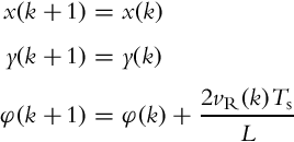
and the straight motion equation (vR(k) = vL(k)) is
So for the desired robot motion inside time interval t ∈ [kTs, (k + 1)Ts) the inverse kinematics can be calculated for each sample time by expressing control variables from Eqs. (2.10), (2.11).
As already stated, there are many other solutions to drive the robot to the desired pose using smooth changing trajectories. The inverse kinematic problem is easier for the desired smooth target trajectory (x(t), y(t)) that the robot should follow so that its orientation is always tangent to the trajectory. Trajectory is defined in time interval t ∈ [0, T]. Supposing the robot’s initial pose is on trajectory, and there is a perfect kinematic model and no disturbances, we can calculate required control variables v as follows:
where the sign depends on the desired driving direction (+ for forward and − for reverse). The tangent angle of each point on the path is defined as
where l ∈{0, 1} defines the desired driving direction (0 for forward and 1 for reverse) and the function arctan2 is the four-quadrant inverse tangent function. By calculating the time derivative of Eq. (2.13) the robot’s angular velocity ω(t) is obtained:
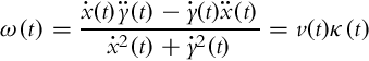
where κ(t) is the path curvature. Using relations (2.12), (2.14) and the defined desired robot path x(t), y(t), the robot control inputs v(t) and ω(t) are calculated. The necessary condition in the path-design procedure is a twice-differentiable path and a nonzero tangential velocity v(t)≠0. If for some time t the tangential velocity is v(t) = 0, the robot rotates at a fixed point with the angular velocity ω(t). The angle φ(t) cannot be determined from Eq. (2.12), and therefore, φ(t) must be given explicitly. Usually this approach is used to determine the feedforward part of the control supplementary to the feedback part which takes care of the imperfect kinematic model, disturbances, and the initial pose error [4].
2.2.2 Bicycle Drive
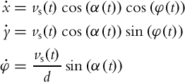
Bicycle drive is shown in Fig. 2.4. It has a steering wheel where α is the steering angle and ωS is wheel angular velocity around its axis (front-wheel drive). The ICR point is defined by the intersection of both wheel axes. In each moment of time the bicycle circles around ICR with angular velocity ω, radius R, and distance between the wheels d:

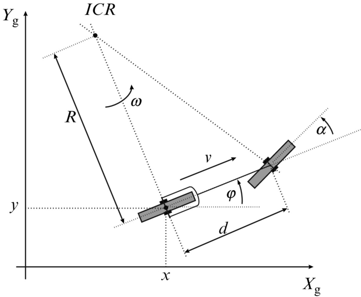
The steering wheel circles around ICR with ω so we can write
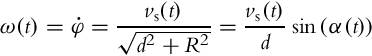
where vs(t) = ωs(t)r and r are the rim velocity and the radius of the front wheel, respectively.
Internal robot kinematics (in robot frame) is
and the external kinematic model is

or in compact form
where ![]() and
and ![]() .
.
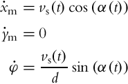
Rear-Wheel Bicycle Drive
Usually vehicles are powered by the rear wheels and steered by the front wheel (e.g., bicycle, tricycles, and some cars). The control variables in this case are rear velocity vr(t) and steering angle of the front wheel α(t). The internal kinematic model can simply be derived from Eq. (2.15) where substituting ![]() leads to the following:
leads to the following:
and the external kinematic model becomes
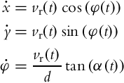
or in equivalent matrix form

where ![]() .
.
Direct and Inverse Kinematics
Considering Eq. (2.17) bicycle direct kinematics (front-wheel drive case) is obtained by Eq. (2.4) similarly as in the case of differential drive.
Inverse kinematics is in general very difficult to solve unless a special case of motion strategy with two motion patterns is applied as follows. By the first motion pattern the robot can only move straight ahead (α(t) = 0) and by the second motion pattern the robot can rotate in the spot (![]() ). For the straight motion robot, velocities simplify to v(t) = vs(t) and ω(t) = 0. By inserting these velocities to Eq. (2.17) and discretization, the motion equations reduce to
). For the straight motion robot, velocities simplify to v(t) = vs(t) and ω(t) = 0. By inserting these velocities to Eq. (2.17) and discretization, the motion equations reduce to
For rotation at the spot robot velocities simplify to v(t) = 0 and ![]() . After inserting these velocities to Eq. (2.17) and discretization the motion model is given by
. After inserting these velocities to Eq. (2.17) and discretization the motion model is given by
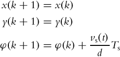
Control variables can be expressed from Eqs. (2.21), (2.22) for required motion during each sample time.
2.2.3 Tricycle Drive
Tricycle drive (see Fig. 2.5) has the same kinematics as bicycle drive.
where ![]() ,
, ![]() , and vs is the rim velocity of the steering wheel.
, and vs is the rim velocity of the steering wheel.
Tricycle drive is more common in mobile robotics because of the three wheels that make the robot stable in a vertical direction by itself.
2.2.4 Tricycle With a Trailer
The tricycle part of kinematics is already described in Section 2.2.3. For a trailer ICR2 is found by the intersection of the tricycle and the trailer wheel axes. The angular velocity at which the trailer wheels circle around the ICR2 point is
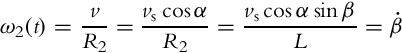
The final kinematic model (for Fig. 2.6) is then obtained as follows:
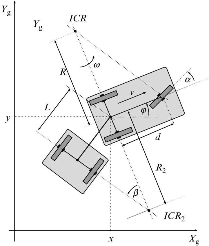
2.2.5 Car (Ackermann) Drive
Cars use the Ackermann steering principle. The idea behind the Ackermann steering is that the inner wheel (closer to ICR) should steer for a bigger angle than the outer wheel in order to allow the vehicle to rotate around the middle point between the rear wheel axis. Consequently the inner wheel travels with a slower speed than the outer wheel. The Ackermann driving mechanism allows for the rear wheels to have no slip angle, which requires that the ICR point lies on a straight line defined by the rear wheels’ axis. This driving mechanism therefore minimizes tire wear.
In Fig. 2.7 the left wheel is on the outer side and the right wheel is on the inner side. The steering orientations of the front wheels are therefore determined from
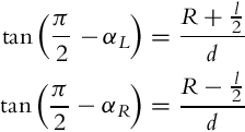
and the final steering angles are expressed as

The inner and outer back wheels circle around the ICR with the same angular velocity ω; therefore their rim velocities are
This type of kinematic drive is especially appropriate to model larger vehicles. A motion model can also be described using tricycle kinematics (Eq. 2.23) where the average the Ackermann angle ![]() is used.
is used.
Inverse kinematics of Ackermann drive is complicated and exceeds the scope of this work.
2.2.6 Synchronous Drive
If a vehicle is able to steer each of its wheels around the vertical axis synchronously (wheels have the same orientation and are steered synchronously) then this is called synchronous drive (also synchro drive). Typical synchro drive has three wheels arranged symmetrically (equilateral triangle) around the vehicle center as in Fig. 2.8.
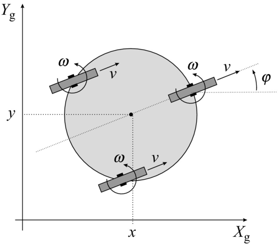
All wheels are synchronously steered so their rotation axes are always parallel and the ICR point is at infinity. The vehicle can directly control the orientation of the wheels, which presents the third state in the state vector (2.27). The control variables are wheels’ steering velocity ω, and forward speed v.
The kinematics has a similar form as in the case of differential drive:
where v(t) and ω(t) (steering velocity of the wheels) are the control variables that can be controlled independently (which is not the case for differential drive).
Forward and Inverse Kinematics
Forward kinematics is obtained by integration of the kinematic model (2.27):
The general solution to the inverse kinematics is not possible because there exists many possible solutions to arrive at the desired pose. However, the inverse kinematics can be solved for a special case where the robot either rotates at the spot or moves straight in its current direction. When the robot rotates at the spot with the constant ω for some time Δt, its orientation changes for ωΔt. In the case of straight motion for some time Δt, with a constant forward velocity v, the robot moves for vΔt in the direction of its current orientation.
2.2.7 Omnidirectional Drive
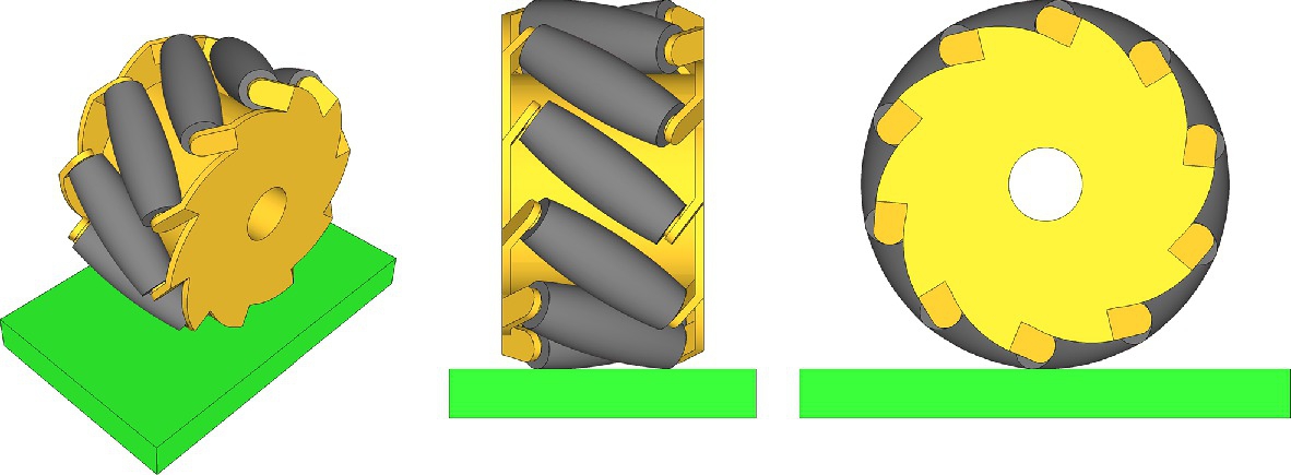
In previous kinematic models simple wheels were used where the wheel can only move (roll) in the direction of its orientation. Such simple wheels have only one rolling direction. To allow omnidirectional rolling motion (in more directions) a complex wheel construction is required. An example of such a wheel is the Mecanum wheel (see Fig. 2.9) or Swedish wheel where the number of smaller rollers are arranged around the main wheel rim. The passive roller axes are not aligned with the main wheel axis (typically they are at a γ = 45 degree angle). This allows a number of different motion directions that result from an arbitrary combination of the main wheel’s rotation direction and passive rollers’ rotation.
Kinematics of Four-Wheel Omnidirectional Drive
Another example of a complex wheel is the omni wheel or poly wheel, which enables omnidirectional motion similarly to the Mecanum wheel. The omni wheel (Fig. 2.10) has passive rollers mounted around the wheel rim so that their axes are 90 degree to the wheel axis.

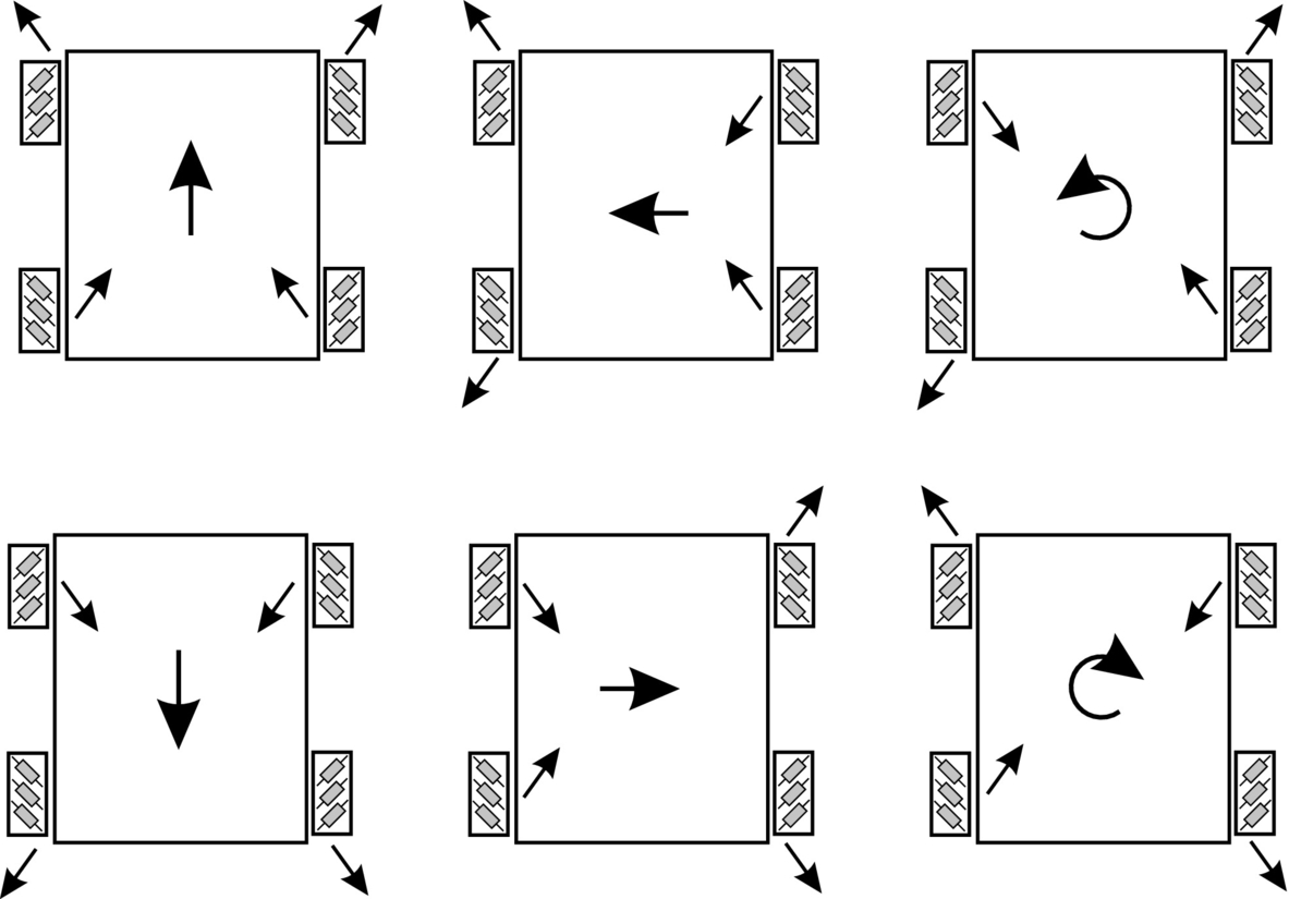
The popular four-wheel platform known as the Mecanum platform is shown in Fig. 2.11. The Mecanum platform has wheels with left- and right-handed rollers where diagonal wheels are of the same type. This enables the vehicle to move in any direction with arbitrary rotation by commanding a proper velocity to each main wheel. Forward or backward motion is obtained by setting all main wheels to the same velocity. If velocities of the main wheels on one side are opposite to the velocities of the wheels on the other side then the platform will rotate. Side motion of the platform is obtained if the wheels on one diagonal have opposite velocity to the wheels on the other diagonal. With combination of the motions described, motion of the platform in any direction and with any rotation can be achieved.
The inverse internal kinematics of the four-wheel Mecanum drive in Fig. 2.12 can be derived as follows.
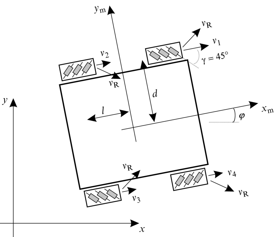
The first wheel velocity in robot coordinates is obtained from the main wheel velocity v1(t) and the passive roller’s velocity vR(t). In the sequel the time dependency notation is omitted to have more compact and easy-to-follow equations (e.g., v1(t) = v1). The total wheel velocity in xm and ym direction of the robot coordinate frame are ![]() and
and ![]() , from where the main wheel velocity is obtained: v1 = vm1x − vm1y. The first wheel velocity in the robot coordinate frame direction can also be expressed with the robot’s translational velocity
, from where the main wheel velocity is obtained: v1 = vm1x − vm1y. The first wheel velocity in the robot coordinate frame direction can also be expressed with the robot’s translational velocity ![]() and its angular velocity
and its angular velocity ![]() as follows:
as follows: ![]() and
and ![]() (the meaning of distances d and l can be deduced from Fig. 2.12). From the latter relations the main wheel velocity can be expressed by the robot body velocity as
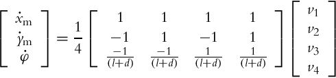
(the meaning of distances d and l can be deduced from Fig. 2.12). From the latter relations the main wheel velocity can be expressed by the robot body velocity as ![]() . Similar equations can be obtained for v2, v3, and v4. The inverse kinematics in local coordinates is
. Similar equations can be obtained for v2, v3, and v4. The inverse kinematics in local coordinates is

The internal inverse kinematics (Eq. 2.29) in compact form reads ![]() , where vT = [v1, v2, v3, v4]T and qmT = [xm, ym, φ]T.
, where vT = [v1, v2, v3, v4]T and qmT = [xm, ym, φ]T.
To calculate the inverse kinematics in global coordinates the rotation matrix representing the orientation of the local coordinates with respect to the global coordinates (![]() ),
),

needs to be considered as follows: ![]() .
.
From the internal inverse kinematics ![]() (Eq. 2.29), the forward internal kinematics is obtained by
(Eq. 2.29), the forward internal kinematics is obtained by ![]() , where
, where ![]() is the pseudo-inverse of J. Forward internal kinematics for the four-wheel Mecanum platform reads as follows:
is the pseudo-inverse of J. Forward internal kinematics for the four-wheel Mecanum platform reads as follows:
Forward kinematics in global coordinates is obtained by ![]() .
.
Kinematics of Three-Wheel Omnidirectional Drive
A popular omnidirectional configuration for three-wheel drive is shown in Fig. 2.13.
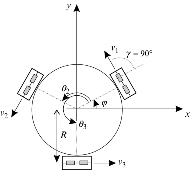
Its inverse kinematics (in global coordinates) is obtained by considering the robot translational velocity ![]() and its angular velocity
and its angular velocity ![]() . Velocity of the first wheel v1 = v1t + v1r consists of a translational part
. Velocity of the first wheel v1 = v1t + v1r consists of a translational part ![]() and an angular part
and an angular part ![]() . The first wheel common velocity therefore is
. The first wheel common velocity therefore is ![]() . Similarly, considering the global angle of the second wheel φ + θ2, its velocity is
. Similarly, considering the global angle of the second wheel φ + θ2, its velocity is ![]() . And the velocity of the third wheel reads
. And the velocity of the third wheel reads ![]() . The inverse kinematics in global coordinates of three-wheel drive is
. The inverse kinematics in global coordinates of three-wheel drive is
The inverse kinematics (Eq. 2.31) in compact form reads ![]() . Sometimes it is more convenient to steer the robot in its local coordinates, which can be obtained by considering rotation transformation as follows:
. Sometimes it is more convenient to steer the robot in its local coordinates, which can be obtained by considering rotation transformation as follows: ![]() .
.
Forward kinematics in global coordinates is obtained from the inverse kinematics (Eq. 2.31) by ![]() where S =J−1:
where S =J−1:
2.2.8 Tracked Drive
The kinematics of the tracked drive (Fig. 2.14) can be approximately described by the differential drive kinematics.
However, the differential drive assumes perfect rolling contact between its wheels and the ground, which is not the case for tracked drive. The tracked drive (Caterpillar tractor) has a bigger contact surface between its wheels and the ground and requires wheels slipping to change its direction. The tracked drives can therefore move through more rough terrain where wheeled vehicles usually cannot.
The amount of sleep between the Caterpillar tractor and the ground is not constant and depends on ground contact; therefore the odometry (direct kinematics) is even less reliable to estimate the robot pose compared to the differential drive.
2.3 Motion Constraints
Motion of WMR is constrained by dynamic and kinematic constraints. Dynamic constraints have origin in the system dynamic model where the system’s response is limited due to its inertia or constraints of the actuators (e.g., limited torque of the motor drive due to its capabilities or to prevent wheel slipping). Kinematic constraints have origin in robot construction and its kinematic model. Kinematic constraints can be holonomic or nonholonomic. Nonholonomic constraints limit some driving directions of a mobile robot [5]. Holonomic constraints are related to the dimensionality of the system state description (generalized coordinates). If holonomic constraints are present, then some coordinates of the state description depend on the others and can therefore be used to eliminate those coordinates from the system’s state description.
A system is holonomic if it has no kinematic constraints or if it only has holonomic constraints. Holonomic systems have no limitation in their velocity space so all directions of motion in the state space are possible. The system is nonholonomic if it has nonholonomic constraints and therefore it cannot move in arbitrary direction (e.g., a car can only move forwards or backwards and not in the lateral direction). For holonomic systems one can determine a subset of independent generalized coordinates which defines a space in which all directions of motion are possible. For noholonomic systems the motion of the system is not arbitrary; nonholonomic constraints define a subspace of possible velocity space in the current moment.
In holonomic systems their state directly depends on the configuration of the system’s internal variables (wheel rotation, joint’s angles). In nonholonomic systems the latter is not true because the returning of the system’s internal variables to the initial values does not guarantee that the system will return to its initial state. The state of the nonholonomic system therefore depends on the traveled path (the sequence of the internal variables).
In the following, mechanical systems will be described whose configuration (system pose in the environment and relation of the systems parts) can be described by the vector of generalized coordinates q. At some given trajectory q(t) a vector of generalized velocities is defined by ![]() .
.
Holonomic constraints are expressed by equations that contain generalized coordinates. These equations can be used to eliminate some generalized coordinates in the effort to obtain a smaller set of required generalized coordinates for some system description. Noholonomic constraints do not reduce the generalized coordinate’s dimension but only the dimension of generalized velocity space. Nonholonomic constraints therefore affect the path planning problem. Regarding nonholonomic constraints the following questions appear:
• How are nonholonomic constraints identified? If a constraint is integrable, then its velocity dependence can be integrated and expressed by a holonomic constraint.
• Does a nonholonomic constraint limit the space of reachable configurations (e.g., system pose)? No, with the use of control theory tools simple conditions are obtained under which arbitrary configuration can be obtained.
• How can a feasible path generator for a nonholonomic robot be constructed?
2.3.1 Holonomic Constraints
These constraints depend on generalized coordinates. For a system with n generalized coordinates q = [q1, …, qn]T a holonomic constraint is expressed in the following form:
where f and its derivatives are continuous functions. This constraint defines a subspace of all possible configurations in generalized coordinates for which Eq. (2.34) is true. Constraint (2.34) can be used to eliminate certain generalized coordinates (it can be expressed by n − 1 other coordinates).
In general we can have m holonomic constraints (m < n). If these constraints are linearly independent then they define (n − m)-dimensional subspace, which is true configuration space (work space, system has n − m DOFs).
2.3.2 Nonholonomic Constraints
Nonholonomic constraints limit possible velocities of the system or possible directions of motion. The nonholonomic constraint can be formulated by
where f is a smooth function with continuous derivatives and ![]() is the vector of system velocities in the generalized coordinates. In case the system has no constraints (2.35), it has no limitation in motion directions.
is the vector of system velocities in the generalized coordinates. In case the system has no constraints (2.35), it has no limitation in motion directions.
A kinematic constraint (2.35) is holonomic if it is integrable, which means that velocities ![]() can be eliminated from Eq. (2.35) and the constraint can be expressed in the form of Eq. (2.34). If the constraint (2.35) is not integrable, then it is nonholonomic.
can be eliminated from Eq. (2.35) and the constraint can be expressed in the form of Eq. (2.34). If the constraint (2.35) is not integrable, then it is nonholonomic.
If m linearly independent nonholonomic constraints exist in the form Eq. (2.35), the velocity space is (n − m)-dimensional. Nonholonomic constraints limit allowable velocities of the system. For example, a differential drive vehicle (e.g., wheelchair) can move in the direction of the current wheel orientation but not in the lateral direction.
Assuming linear constraints in ![]() , Eq. (2.35) can be written as
, Eq. (2.35) can be written as

where a(q) is a parameter vector of the constraint. For m nonholonomic constraints a constraint matrix is obtained as follows:
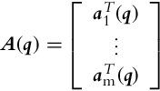
and all nonholonomic constraints are given in matrix form
In each time instant a matrix of reachable motion directions is S(q) = [s1(q), …, sn−m(q)] (m constraints define (n − m) reachable directions). This matrix defines the kinematic model as follows:
where v(t) is the control vector (see kinematic model (2.2)). The product of the constraint matrix A and the kinematic matrix S is a zero matrix:
2.3.3 Integrability of Constraints
To determine if some constraint is nonholonomic, an integrability test needs to be done. If it cannot be integrated to obtain the form of holonomic constraint, the constraint is nonholonomic.
2.3.4 Vector Fields, Distribution, Lie Bracket
In current time t and current state q all possible motion directions can be obtained by a linear combination of vector fields in matrix S. Distribution is defined as a reachable subspace from q using motions defined by a linear combination of vector fields (columns in S).
Vector fields are time derivatives of generalized coordinates and therefore represent velocities or motion directions. A vector field is a mapping that is continuously differentiable and assigns a specific vector to each point in state space. A demonstration of reachable vector field determination for differential drive is given in Example 2.1.
Example 2.1
For a differential drive robot with kinematic model (2.2), define reachable velocities (motion directions) and motion constraints.
Solution
The vector fields of reachable velocities (motion directions) are defined as
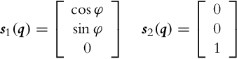
This means that all possible motion directions in current time at the current pose q are obtained by the linear combination
where u1 in u2 are arbitrary real numbers that represent the control inputs. Eq. (2.42) can be seen as an alternative form of the kinematic model (2.2).
If vector fields si are not given, they can be obtained from known constraints aj considering the fact that constraint directions are orthogonal to the motion directions, so si⊥aj. In Fig. 2.3 the constraint can be determined by identifying the directions where the robot cannot move; this is in the direction lateral to the wheels. The only constraint is
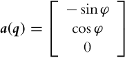
which is perpendicular to the motion direction vector s1(q) (longitudinal motion in the direction of the wheels rotation) and to the vector s2(q) (rotation around axis normal to the surface).
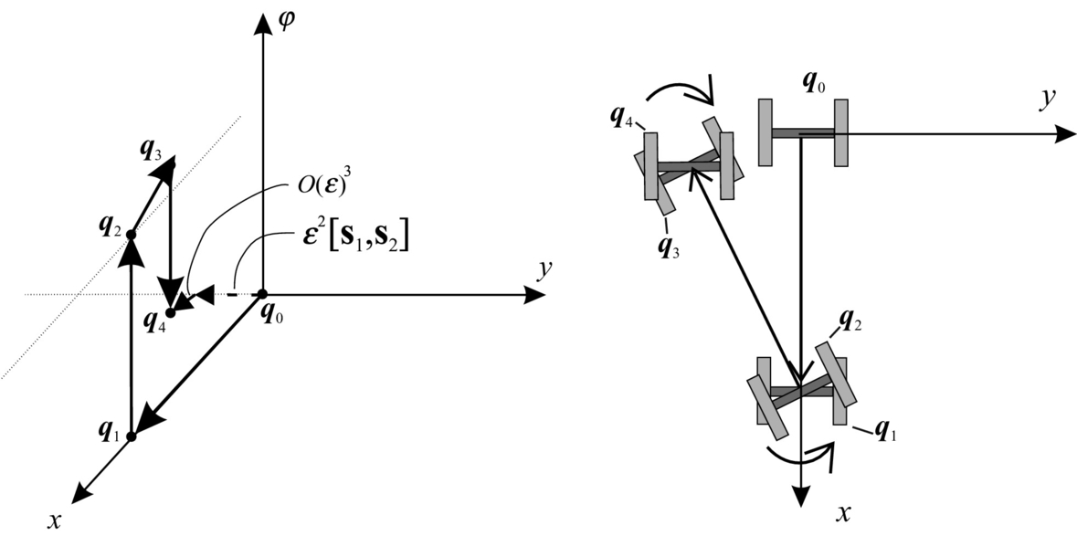
If distribution of some vector fields span the whole space then it is involutive. For noninvolutive distribution of some vector fields a set of new vector fields (linearly independent from vector fields of the basic distribution) can be defined. These new vector fields (motion directions) can be obtained by a finite switching of the basic motion directions with movement length (in each basic direction) limited to zero. New motion directions can be calculated using Lie brackets, which operates over two vector fields as shown later in Eq. (2.44). Parallel parking of a car or differential drive is a practical example of obtaining a new motion direction by switching between the basic motion directions. The car cannot directly move in the lateral direction to the parking slot. However, it can still go into a parking slot by lateral direction movement from a series of forward, backward, and rotation motions as illustrated in Example 2.2.
Example 2.2
Illustration of parallel parking maneuver of differential drive vehicle.
Solution
Using the basic motion directions defined by the vector fields s1(q) and s2(q) (see Eq. 2.41) and the initial vehicle pose q0 = q(0) new vehicle poses are obtained as follows. Starting from q0 = q(0) and driving in the direction s1 for a short period of time ε, then driving in the direction s2 for time ε followed by driving in the direction −s1 for time ε, and finally for time ε in the direction −s2, the final pose is obtained. Mathematically this is formulated as follows:
which represents a nonlinear differential equation whose solution can be approximated by Taylor series expansion (see details in [1]) by

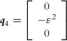
where partial derivatives are estimated for q0 and O(ε3) is the remaining part belonging to a higher order of derivatives that can be ignored for a short time ε. The obtained final motion distance of the parallel parking maneuver is ε2 in the direction of the vector obtained by Lie brackets (defined in Eq. 2.44).
Illustration of this maneuver can be done by the following experiment. Suppose the starting vehicle pose is q0 = [0, 0, 0]T. By performing the first step of the parking maneuver the resulting pose is
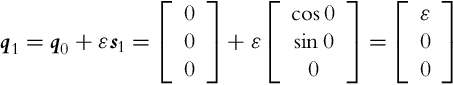
In the second step a rotation is performed

The third step contains translation in the negative direction:
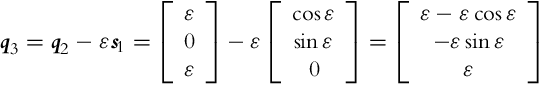
and in the last step there is a rotation in the negative direction:
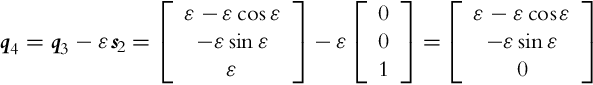
Computed motions and intermediate points are shown in Fig. 2.15. The final pose of this maneuver is in the lateral direction to the starting pose. The final pose, however, is not directly accessible with basic motion vector fields s1 and s2, but it can be achieved by a combination of the basic vector fields. The obtained final motion is not strictly in the lateral direction due to the final time ε and part O(ε3) in Eq. (2.43). In limit case when each motion time duration ![]() the obtained final pose is exactly in the lateral direction.
the obtained final pose is exactly in the lateral direction.
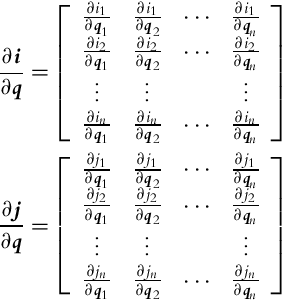
As seen from Example 2.2 the Lie brackets can be used to identify new motion directions that are not allowed by the basic distribution. This new motion directions can be achieved by a finite number of infinitely small motions in directions from the basic vector field’s distribution. A Lie bracket is operating over two vector fields i(q) and j(q), and the result is a new vector field [i, j] obtained as follows:

where
Distribution is involutive if new linearly independent vector fields cannot be obtained using Lie brackets over the existing vector fields in the distribution. If distribution is involutive then it is closed under Lie brackets [6]. Then the system is completely holonomic with no motion constraints or only with holonomic constraints. This statement is explained by the Frobenious theorem [7]: If basic distribution is involutive then the system is holonomic and all existing constraints are integrable. Let us suppose that from m constraints, k constraints are holonomic and (m − k) nonholonomic. According to the Frobenious theorem there are three possibilities for k [8]:
• k = m, which means that the dimension of involutive distribution is (n − m), which also equals to the dimension of the basic distribution. Distribution dimension equals the number of linearly independent vector fields.
• 0 < k < m, k constraints are integrable, so k generalized coordinates can be eliminated from the system description. The dimension of involutive distribution is n − k.
• k = 0, the dimension of involutive distribution is n, and all constraints are nonholonomic.
Example 2.3
For a wheel rolling on a plane, determine motion constraints and vector fields of possible motion directions. Determine the system’s DOF and the number and type of its constraints.
Solution
The kinematic model of the wheel is the same as for the differential drive given in Fig. 2.3 and in kinematic model (2.2). Constrained motion directions and possible motion directions have already been determined in Example 2.1. We have one velocity constraint, which does not limit the accessibility of states q, and therefore the system has three DOFs. To prove that there is a velocity constraint (nonholonomic) Lie brackets and the Frobenious theorem could be used.
Using reachable basic vector fields s1 and s2 and determining the new vector field by Lie brackets (Eq. 2.41), the following is found:
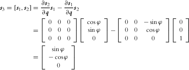
A new possible direction of motion is obtained that is linearly independent from the vector fields s1 and s2 and therefore not present in the basic distribution. Therefore we can conclude that the constraint is nonholonomic; the dimension of involutive distribution is 3 (system has 3 DOFs), which is the same as the dimension of the system. It is also not possible to generate new linearly independent vector fields using additional Lie brackets ([s1, s3], [s2, s3]).
Example 2.4
Determine motion constraints and directions of possible motion for a car-like vehicle without a (or with a locked) steering mechanism (Fig. 2.16). Find out the number and the type of constraints and the system’s DOF.
Solution
The vehicle cannot move in the lateral direction and it cannot rotate (its orientation φ is fixed); therefore constraint motion directions are

and the motion constraints are

Both constraints are integrable, which can simply be seen by calculating their integral:
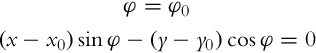
The vehicle can only move in the direction of the vector field:

Because both constraints are holonomic the distribution of the vector field s1 is involutive, meaning that the system is completely holonomic and the system has 1 DOF. Using Lie brackets it is not possible to generate new vector fields as we have only one vector field that defines possible motion.
Example 2.6
Using Matlab perform a simulation of a tricycle drive (rear-powered) platform. The vehicle parameters are the following: sampling period Ts = 0.033 s, time of simulation 10 s, wheel radius R = 0.2 m, distance between the wheels L = 0.08 m, and distance between the front and rear wheels D = 0.07 m.
Tasks:
1. Calculate analytically and by means of simulation the shape of the path made by the robot if the initial state is q(0) = [x, y, φ]T = [0, −0.5, 0]T and robot inputs in two cases are the following:
• v(t) = 0.5 m/s, α(t) = 0
• v(t) = 1 m/s, ![]()
What are the wheels’ angular speeds? Is the calculated and simulated path the same. Why or why not?
2. Implement localization of the vehicle at constant input speeds (v(t) = 0.5 m/s, ![]() ) using odometry. Compare the estimated path with the simulated path of the true robot. Compare the obtained results also in the ideal situation without noise and modeling error.
) using odometry. Compare the estimated path with the simulated path of the true robot. Compare the obtained results also in the ideal situation without noise and modeling error.
3. Repeat the localization from question 2 also with initial state error (suppose the true initial state is unknown; therefore choose initial state in localization different than in simulation).
4. Imagine a path composed of two or three straight line segments where the initial point coincides with the initial robot pose. Calculate the required sequence of inputs to drive the robot on that path (time of simulation is 10 s).
5. Choose some trajectory defined as parametric functions of time (x(t) = f(t) and y(t) = g(t)), where f and g are smooth functions. Calculate required inputs to follow this path. What happens if the robot initially is not on the trajectory?
2.3.5 Controllability of Wheeled Mobile Robots
Before designing motion control we need to find the answer to the following question: Can the robot reach any point q in the configuration space by performing its available maneuvers? The answer to this question is related to the controllability of the system. If the system is controllable, it can reach any configuration q by combining available motion maneuvers.
If the robot has kinematic constraints then we need to analyze them and figure out if they affect the system controllability. The robot with nonholonomic constraints can only move in its basic motion directions (basic maneuvers like driving straight and rotating) but not in the constrained direction. However, such robot may still achieve any desired configuration q by combining basic maneuvers. New direction of motion is different than any basic direction or any linear combination of the basic directions as given in Eq. (2.39). Controllability of the robot is determined by analyzing the involutive (accessibility) distribution obtained by successive Lie bracket operations over the basic motion directions s1, s2, s3, …as follows [7, 9–12]:
If the rank of the involutive distribution is n (n is the dimension of q) then the robot can reach any point q in the configuration space and is therefore controllable. The latter statement is also known as Chow’s theorem: The system is controllable if its involutive distribution regarding Lie brackets has rank equal to the dimension of the configuration space. Some robots are controllable if all their constraints are nonholonomic and if their involutive distribution has rank n. This controllability test is for nonlinear systems but can also be applied to linear systems ![]() , where the basic vector fields are s1 = Aq and s2 = B. Calculating the involutive distribution results in the Kalman test for controllability of the linear systems:
, where the basic vector fields are s1 = Aq and s2 = B. Calculating the involutive distribution results in the Kalman test for controllability of the linear systems:
To obtain involutive distribution successive levels of Lie brackets are calculated. The number of those successive levels defines the difficulty index of maneuvering the WMR platform [13]. The higher the difficulty index, the higher the number of the basic maneuvers required to achieve any desired motion direction.
Example 2.7
Show that the differential drive is controllable.
Solution
Differential drive has three states (n = 3) q = [x, y, φ] and two basic motion directions s1 and s2:
The new motion direction obtained by the Lie bracket is

Calculating Lie brackets from any combination of s1, s2, and s3 does not produce a new linearly independent motion direction; therefore the distribution [s1, s2, s3] is involutive (closed by Lie brackets) and has rank:
so the system is controllable.
Example 2.8
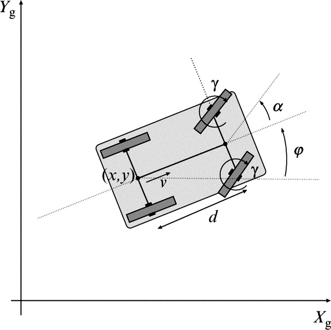
Determine motion constraints and possible motion directions for a rear-powered car. The car can be controlled by the rim velocity of the rear wheels v and by the angular speed of the steering mechanism γ (Fig. 2.17).
Find out the number and the type of motion constraints, the kinematic model, and the number of DOFs. Is the system controllable?
Solution
The vehicle configuration can be described by four states q = [x, y, φ, α]T, because the control inputs are velocity v and the angular velocity of the steering mechanism γ. The fourth state (![]() ) therefore describes the current state of the steering.
) therefore describes the current state of the steering.
Note that bicycle kinematics with rear wheel drive has the same kinematics (Eq. 2.19) as the car in this example, but it has only three states because the angle of the steering mechanism is already defined by one of the inputs in Eq. (2.19).
The vehicle cannot move laterally to the rear and front wheels; therefore the motion constraints are

Vector fields that define the basic motion directions are defined by the rolling direction of the rear wheels (direction of motion when γ = 0, which means constant α) and by the rotation of the steering wheels (direction of motion when v = 0)
The vehicle kinematic model is defined by
which is similar to kinematics (Eq. 2.19) but with an additional state α and input ![]() .
.
So the system is described by four states; it has two constraints and two inputs. We will try to obtain new linearly independent motion directions si. Two are defined by the kinematic model, and the other two are obtained by Lie brackets:
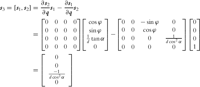
and
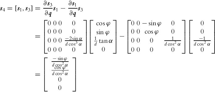
Because all four vector fields si, i = 1, …, 4 are linearly independent the system has four DOFs and both constraints are nonholonomic.
The involutive closure has a rank of 4, which is the number of the system states. The vehicle is therefore controllable.