
Trees and rules
Abstract
This chapter explains practical decision tree and rule learning methods, and also considers more advanced approaches for generating association rules. The basic algorithms for learning classification trees and rules presented in Chapter 4, Algorithms: the basic methods, are extended to make them applicable to real-world problems that contain numeric attributes, noise, and missing values. We discuss the seminal C4.5 algorithm for decision tree learning, consider an alternative pruning method implemented in the CART tree learning algorithm, and discuss the incremental reduced-error pruning method for growing and pruning classification rules, leading up to the RIPPER and PART algorithms for rule induction. We also briefly consider rule sets with exceptions. The last section of this chapter switches to unsupervised learning of rule sets by investigating how a special-purpose data structure can be constructed to accelerate the process of finding association rules. More specifically, we consider frequent-pattern trees and how they can be used to efficiently search for frequent item sets.
Keywords
Decision trees; classification rules; pruning; numeric attributes; missing values; rules with exceptions; association rules; frequent-pattern trees
Decision tree learners are the workhorses of many practical applications of machine learning because they are fast and produce intelligible output that is often surprisingly accurate. This chapter explains how to make decision tree learning robust and versatile enough to cope with the demands of real-world datasets. It shows how to deal with numeric attributes and missing values, and how to prune away those parts of a tree that do not actually enjoy sufficient support from the data. Our discussion is based on how these issues are addressed in the classic C4.5 algorithm for decision tree learning, but we will also see how cross-validation is used by the famous CART decision tree learner to implement a more robust pruning strategy.
The second topic in this chapter is rule learning. When implemented appropriately, this shares the advantages of decision tree learning, at a somewhat higher cost in runtime, and often yields even more concise classification models. Surprisingly, rules are less popular than decision trees in practice—perhaps because rule learning algorithms are quite heuristic and are not often considered outside the artificial intelligence community. We will see how to make the basic rule learning strategy from Chapter 4, Algorithms: the basic methods, less prone to overfitting, how to deal with missing values and numeric attributes, and how to select and prune good rules. Generating concise and accurate rule sets is trickier than learning concise and accurate decision trees. We will discuss two strategies for achieving this: one based on global optimization of a rule set and another based on extracting rules from partially grown and pruned decision trees. We will also briefly look at the advantages of representing learned knowledge using rules sets with exceptions.
6.1 Decision Trees
The first machine learning scheme that we will develop in detail, the C4.5 algorithm, derives from the simple divide-and-conquer algorithm for producing decision trees that was described in Section 4.3. It needs to be extended in several ways before it is ready for use on real-world problems. First we consider how to deal with numeric attributes, and, after that, missing values. Then we look at the all-important problem of pruning decision trees, because trees constructed by the basic divide-and-conquer algorithm as described perform well on the training set, but are usually overfitted to it and do not generalize well to independent test sets. We then briefly consider how to convert decision trees to classification rules, and examine the options provided by the C4.5 algorithm itself. Finally, we look at an alternative pruning strategy that is implemented in the famous CART system for learning classification and regression trees.
Numeric Attributes
The method we described in Section 4.3 only works when all the attributes are nominal, whereas, as we have seen, most real datasets contain some numeric attributes. It is not too difficult to extend the algorithm to deal with these. For a numeric attribute we will restrict the possibilities to a two-way, or binary, split. Suppose we use the version of the weather data that has some numeric features (Table 1.3). Then, when temperature is being considered for the first split, the temperature values involved are
| 64 | 65 | 68 | 69 | 70 | 71 | 72 | 75 | 80 | 81 | 83 | 85 |
| Yes | No | Yes | Yes | Yes | No | No Yes |
Yes Yes |
No | Yes | Yes | No |

(Repeated values have been collapsed together), and there are only 11 possible positions for the breakpoint—8 if the breakpoint is not allowed to separate items of the same class. The information gain for each can be calculated in the usual way. For example, the test temperature < 71.5 produces four yes’s and two no’s, whereas temperature > 71.5 produces five yes’s and three no’s, and so the information value of this test is
It is common to place numeric thresholds halfway between the values that delimit the boundaries of a concept, although something might be gained by adopting a more sophisticated policy. For example, we will see below that although the simplest form of instance-based learning puts the dividing line between concepts in the middle of the space between them, other methods that involve more than just the two nearest examples have been suggested.
When creating decision trees using the divide-and-conquer method, once the first attribute to split on has been selected, a top-level tree node is created that splits on that attribute, and the algorithm proceeds recursively on each of the child nodes. For each numeric attribute, it appears that the subset of instances at each child node must be re-sorted according to that attribute’s values—and, indeed, this is how programs for inducing decision trees are usually written. However, it is not actually necessary to re-sort because the sort order at a parent node can be used to derive the sort order for each child, leading to a speedier implementation, at the expense of storage. Consider the temperature attribute in the weather data, whose sort order (this time including duplicates) is
| 64 | 65 | 68 | 69 | 70 | 71 | 72 | 72 | 75 | 75 | 80 | 81 | 83 | 85 |
| 7 | 6 | 5 | 9 | 4 | 14 | 8 | 12 | 10 | 11 | 2 | 13 | 3 | 1 |

The italicized number below each temperature value gives the number of the instance that has that value: thus instance number 7 has temperature value 64, instance 6 has temperature 65, and so on. Suppose we decide to split at the top level on the attribute outlook. Consider the child node for which outlook=sunny—in fact the examples with this value of outlook are numbers 1, 2, 8, 9, and 11. If the italicized sequence is stored with the example set (and a different sequence must be stored for each numeric attribute)—i.e., instance 7 contains a pointer to instance 6, instance 6 points to instance 5, instance 5 points to instance 9, and so on—then it is a simple manner to read off the examples for which outlook=sunny in order. All that is necessary is to scan through the instances in the indicated order, checking the outlook attribute for each and writing down the ones with the appropriate value:
| 9 | 8 | 11 | 2 | 1 |

Thus repeated sorting can be avoided by storing with each subset of instances the sort order for that subset according to each numeric attribute. The sort order must be determined for each numeric attribute at the beginning; no further sorting is necessary thereafter.
When a decision tree tests a nominal attribute as described in Section 4.3, a branch is made for each possible value of the attribute. However, we have restricted splits on numeric attributes to be binary. This creates an important difference between numeric attributes and nominal ones: once you have branched on a nominal attribute, you have used all the information that it offers, whereas successive splits on a numeric attribute may continue to yield new information. Whereas a nominal attribute can only be tested once on any path from the root of a tree to the leaf, a numeric one can be tested many times. This can yield trees that are messy and difficult to understand because the tests on any single numeric attribute are not located together but can be scattered along the path. An alternative, which is harder to accomplish but produces a more readable tree, is to allow a multiway test on a numeric attribute, testing against several different constants at a single node of the tree. A simpler but less powerful solution is to prediscretize the attribute as described in Section 8.2.
Missing Values
The next enhancement to the decision tree-building algorithm deals with the problems of missing values. Missing values are endemic in real-world datasets. As explained in Chapter 2, Input: concepts, instances, attributes, one way of handling them is to treat them as just another possible value of the attribute; this is appropriate if the fact that the attribute is missing is significant in some way. In that case no further action need be taken. But if there is no particular significance in the fact that a certain instance has a missing attribute value, a more subtle solution is needed. It is tempting to simply ignore all instances in which some of the values are missing, but this solution is often too draconian to be viable. Instances with missing values often provide a good deal of information. Sometimes the attributes whose values are missing play no part in the decision, in which case these instances are as good as any other.
One question is how to apply a decision tree, once it has been constructed, to an instance in which some of the attributes to be tested have missing values. We outlined a solution in Section 3.3. It involves notionally splitting the instance into pieces, using a numeric weighting scheme, and sending part of it down each branch in proportion to the number of training instances going down that branch. Eventually, the various parts of the instance will each reach a leaf node, and the decisions at these leaf nodes must be recombined using the weights that have percolated to the leaves.
A second question, which precedes the first one because it applies to training, is how to partition the training set once a splitting attribute has been chosen, to allow recursive application of the decision tree formation procedure on each of the daughter nodes. The same weighting procedure is used. Instances for which the relevant attribute value is missing are notionally split into pieces, one piece for each branch, in the same proportion as the known instances go down the various branches. Pieces of the instance contribute to decisions at lower nodes in the usual way through the information gain or gain ratio calculation, except that they are weighted accordingly. The calculations described in Section 4.3 can also be applied to partial instances. Instead of having integer counts, the weights are used when computing both gain figures. Instances may be further split at lower nodes, of course, if the values of other attributes are unknown as well.
Pruning
Fully expanded decision trees often contain unnecessary structure, and it is generally advisable to simplify them before they are deployed. Now it is time to learn how to prune decision trees.
By building the complete tree and pruning it afterward we are adopting a strategy of postpruning (sometimes called backward pruning) rather than prepruning (or forward pruning). Prepruning would involve trying to decide during the tree-building process when to stop developing subtrees—quite an attractive prospect because that would avoid all the work of developing subtrees only to throw them away afterward. However, postpruning does seem to offer some advantages. For example, situations occur in which two attributes individually seem to have nothing to contribute but are powerful predictors when combined—a sort of combination-lock effect in which the correct combination of the two attribute values is very informative whereas the attributes taken individually are not. Most decision tree builders postprune.
Two rather different operations have been considered for postpruning: subtree replacement and subtree raising. At each node, a learning scheme might decide whether it should perform subtree replacement, subtree raising, or leave the subtree as it is, unpruned. Subtree replacement is the primary pruning operation, and we look at it first. The idea is to select some subtrees and replace them with single leaves. For example, the whole subtree in Fig. 1.3B, involving two internal nodes and four leaf nodes, has been replaced by the single leaf bad. This will certainly cause the accuracy on the training set to decrease if the original tree is produced by the decision tree algorithm described previously, because that continues to build the tree until all leaf nodes are pure (or until all attributes have been tested). However, it may increase the accuracy on an independently chosen test set.
When subtree replacement is implemented, it proceeds from the leaves and works back up toward the root. In the Fig. 1.3 example, the whole subtree in (b) would not be replaced at once. First, consideration would be given to replacing the three daughter nodes in the health plan contribution subtree with a single leaf node. Assume that a decision is made to perform this replacement—we will explain how shortly. Then, continuing to work back from the leaves, consideration would be given to replacing the working hours per week subtree, which now has just two daughter nodes, by a single leaf node. In the Fig. 1.3 example this replacement was indeed made, which accounts for the entire subtree in (b) being replaced by a single leaf marked bad. Finally, consideration would be given to replacing the two daughter nodes in the wage increase 1st year subtree with a single leaf node. In this case that decision was not made, so the tree remains as shown in Fig. 1.3A. Again, we will examine how these decisions are actually made shortly.
The second pruning operation, subtree raising, is more complex, and it is not clear that it is necessarily always worthwhile. However, because it is used in the influential decision tree building system C4.5, we describe it here. Subtree raising does not occur in the Fig. 1.3 example, so use the artificial example of Fig. 6.1 for illustration. Here, consideration is given to pruning the tree in Fig. 6.1A, and the result is shown in Fig. 6.1B. The entire subtree from C downward has been “raised” to replace the B subtree. Note that although the daughters of B and C are shown as leaves, they can be entire subtrees. Of course, if we perform this raising operation, it is necessary to reclassify the examples at the nodes marked 4 and 5 into the new subtree headed by C. This is why the daughters of that node are marked with primes: 1′, 2′, and 3′—to indicate that they are not the same as the original daughters 1, 2, and 3 but differ by the inclusion of the examples originally covered by 4 and 5.

Subtree raising is a potentially time-consuming operation. In actual implementations it is generally restricted to raising the subtree of the most popular branch. That is, we consider doing the raising illustrated in Fig. 6.1 provided that the branch from B to C has more training examples than the branches from B to node 4 or from B to node 5. Otherwise, if (e.g.) node 4 were the majority daughter of B, we would consider raising node 4 to replace B and reclassifying all examples under C, as well as the examples from node 5, into the new node.
Estimating Error Rates
So much for the two pruning operations. Now we must address the question of how to decide whether to replace an internal node by a leaf (for subtree replacement), or whether to replace an internal node by one of the nodes below it (for subtree raising). To make this decision rationally, it is necessary to estimate the error rate that would be expected at a particular node given an independently chosen test set. We need to estimate the error at internal nodes as well as at leaf nodes. If we had such an estimate, it would be clear whether to replace, or raise, a particular subtree simply by comparing the estimated error of the subtree with that of its proposed replacement. Before estimating the error for a subtree proposed for raising, examples that lie under siblings of the current node—the examples at 4 and 5 of Fig. 6.1—would have to be temporarily reclassified into the raised tree.
It is no use taking the training set error as the error estimate: that would not lead to any pruning because the tree has been constructed expressly for that particular training set. One way of coming up with an error estimate is the standard verification technique: hold back some of the data originally given and use it as an independent test set to estimate the error at each node. This is called reduced-error pruning. It suffers from the disadvantage that the actual tree is based on less data.
The alternative is to try to make some estimate of error based on the training data itself. That is what C4.5 does, and we will describe its method here. It is a heuristic based on some statistical reasoning, but the statistical underpinning is rather weak. However, it seems to work well in practice. The idea is to consider the set of instances that reach each node and imagine that the majority class is chosen to represent that node. That gives us a certain number of “errors,” E, out of the total number of instances, N. Now imagine that the true probability of error at the node is q, and that the N instances are generated by a Bernoulli process with parameter q, of which E turn out to be errors.
This is almost the same situation as we considered when looking at the holdout method in Section 5.2, where we calculated confidence intervals on the true success probability p given a certain observed success rate. There are two differences. One is trivial: here we are looking at the error rate q rather than the success rate p; these are simply related by p+q=1. The second is more serious: here the figures E and N are measured from the training data, whereas in Section 5.2 we were considering independent test data instead. Because of this difference we make a pessimistic estimate of the error rate by using the upper confidence limit rather than stating the estimate as a confidence range.
The mathematics involved is just the same as before. Given a particular confidence c (the default figure used by C4.5 is c=25%), we find confidence limits z such that
where N is the number of samples, f=E/N is the observed error rate, and q is the true error rate. As before, this leads to an upper confidence limit for q. Now we use that upper confidence limit as a (pessimistic) estimate for the error rate e at the node:

Note the use of the + sign before the square root in the numerator to obtain the upper confidence limit. Here, z is the number of standard deviations corresponding to the confidence c, which for c=25% is z=0.69.
To see how all this works in practice, let’s look again at the labor negotiations decision tree of Fig. 1.3, salient parts of which are reproduced in Fig. 6.2 with the number of training examples that reach the leaves added. We use the above formula with a 25% confidence figure, i.e., with z=0.69. Consider the lower left leaf, for which E=2, N=6, and so f=0.33. Plugging these figures into the formula, the upper confidence limit is calculated as e=0.47. That means that instead of using the training set error rate for this leaf, which is 33%, we will use the pessimistic estimate of 47%. This is pessimistic indeed, considering that it would be a bad mistake to let the error rate exceed 50% for a two-class problem. But things are worse for the neighboring leaf, where E=1 and N=2, because the upper confidence limit becomes e=0.72. The third leaf has the same value of e as the first. The next step is to combine the error estimates for these three leaves in the ratio of the number of examples they cover, 6: 2:6, which leads to a combined error estimate of 0.51. Now we consider the error estimate for the parent node, health plan contribution. This covers nine bad examples and five good ones, so the training set error rate is f=5/14. For these values, the above formula yields a pessimistic error estimate of e=0.46. Because this is less than the combined error estimate of the three children, they are pruned away.
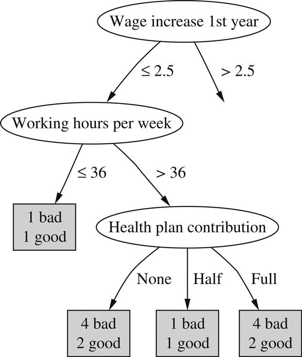
The next step is to consider the working hours per week node, which now has two children that are both leaves. The error estimate for the first, with E=1 and N=2, is e=0.72, while for the second it is e=0.46 as we have just seen. Combining these in the appropriate ratio of 2:14 leads to a value that is higher than the error estimate for the working hours node, so the subtree is pruned away and replaced by a leaf node.
The estimated error figures obtained in these examples should be taken with a grain of salt because the estimate is only a heuristic one and is based on a number of shaky assumptions: the use of the upper confidence limit; the assumption of a normal distribution; and the fact that statistics from the training set are used. However, the qualitative behavior of the error formula is correct and the method seems to work reasonably well in practice. If necessary, the underlying confidence level, which we have taken to be 25%, can be tweaked to produce more satisfactory results.
Complexity of Decision Tree Induction
Now that we have learned how to accomplish the pruning operations, we have finally covered all the central aspects of decision tree induction. Let’s take stock and examine the computational complexity of inducing decision trees. We will use the standard order notation: ![]() stands for a quantity that grows at most linearly with n,
stands for a quantity that grows at most linearly with n, ![]() grows at most quadratically with n, and so on.
grows at most quadratically with n, and so on.
Suppose the training data contains n instances and m attributes. We need to make some assumption about the size of the tree, and we will assume that its depth is on the order of log n, i.e., O(log n). This is the standard rate of growth of a tree with n leaves, provided that it remains “bushy” and does not degenerate into a few very long, stringy branches. Note that we are tacitly assuming that most of the instances are different from each other, and—this is almost the same thing—that the m attributes provide enough tests to allow the instances to be differentiated. For example, if there were only a few binary attributes, they would allow only so many instances to be differentiated and the tree could not grow past a certain point, rendering an “in the limit” analysis meaningless.
The computational cost of building the tree in the first place is
Consider the amount of work done for one attribute over all nodes of the tree. Not all the examples need to be considered at each node, of course. But at each possible tree depth, the entire set of n instances must be considered. And because there are ![]() different depths in the tree, the amount of work for this one attribute is
different depths in the tree, the amount of work for this one attribute is ![]() . At each node all attributes are considered, so the total amount of work is
. At each node all attributes are considered, so the total amount of work is ![]() .
.
This reasoning makes some assumptions. If some attributes are numeric, they must be sorted, but once the initial sort has been done there is no need to re-sort at each tree depth if the appropriate algorithm is used (described earlier). The initial sort takes ![]() operations for each of up to m attributes: thus the above complexity figure is unchanged. If the attributes are nominal, all attributes do not have to be considered at each tree node—because attributes that are used further up the tree cannot be reused. However, if attributes are numeric, they can be reused and so they have to be considered at every tree level.
operations for each of up to m attributes: thus the above complexity figure is unchanged. If the attributes are nominal, all attributes do not have to be considered at each tree node—because attributes that are used further up the tree cannot be reused. However, if attributes are numeric, they can be reused and so they have to be considered at every tree level.
Next, consider pruning by subtree replacement. First an error estimate must be made for every tree node. Provided that counts are maintained appropriately, this is linear in the number of nodes in the tree. Then each node needs to be considered for replacement. The tree has at most n leaves, one for each instance. If it were a binary tree, each attribute being numeric or two-valued, that would give it 2n−1 nodes; multiway branches would only serve to decrease the number of internal nodes. Thus the complexity of subtree replacement is
Finally, subtree lifting has a basic complexity equal to subtree replacement. But there is an added cost because instances need to be reclassified during the lifting operation. During the whole process, each instance may have to be reclassified at every node between its leaf and the root, i.e., as many as ![]() times. That makes the total number of reclassifications
times. That makes the total number of reclassifications ![]() . And reclassification is not a single operation: one that occurs near the root will take
. And reclassification is not a single operation: one that occurs near the root will take ![]() operations, and one of average depth will take half of this. Thus the total complexity of subtree lifting is as follows:
operations, and one of average depth will take half of this. Thus the total complexity of subtree lifting is as follows:
Taking into account all these operations, the full complexity of decision tree induction is
From Trees to Rules
It is possible to read a set of rules directly off a decision tree, as noted in Section 3.4, by generating a rule for each leaf and making a conjunction of all the tests encountered on the path from the root to that leaf. This produces rules that are unambiguous in that it does not matter in what order they are executed. However, the rules are more complex than necessary.
The estimated error rate described previously provides exactly the mechanism necessary to prune the rules. Given a particular rule, each condition in it is considered for deletion by tentatively removing it, working out which of the training examples are now covered by the rule, calculating from this a pessimistic estimate of the error rate of the new rule, and comparing this with the pessimistic estimate for the original rule. If the new rule is better, delete that condition and carry on, looking for other conditions to delete. Leave the rule when there are no conditions left that will improve it if they are removed. Once all rules have been pruned in this way, it is necessary to see if there are any duplicates and remove them from the rule set.
This is a greedy approach to detecting redundant conditions in a rule, and there is no guarantee that the best set of conditions will be removed. An improvement would be to consider all subsets of conditions, but this is usually prohibitively expensive. Another solution might be to use an optimization technique such as simulated annealing or a genetic algorithm to select the best version of this rule. However, the simple greedy solution seems to produce quite good rule sets.
The problem, even with the greedy method, is computational cost. For every condition that is a candidate for deletion, the effect of the rule must be reevaluated on all the training instances. This means that rule generation from trees tends to be very slow, and Section 6.2: Classification Rules describes much faster methods that generate classification rules directly without forming a decision tree first.
C4.5: Choices and Options
C4.5 works essentially as described in the “From Trees to Rules” sections. The default confidence value is set at 25% and works reasonably well in most cases; possibly it should be altered to a lower value, which causes more drastic pruning, if the actual error rate of pruned trees on test sets is found to be much higher than the estimated error rate. There is one other important parameter whose effect is to eliminate tests for which almost all of the training examples have the same outcome. Such tests are often of little use. Consequently tests are not incorporated into the decision tree unless they have at least two outcomes that have at least a minimum number of instances. The default value for this minimum is 2, but it is controllable and should perhaps be increased for tasks that have a lot of noisy data.
Another heuristic in C4.5 is that candidate splits on numeric attributes are only considered if they cut off a certain minimum number of instances: at least 10% of the average number of instances per class at the current node, or 25 instances, whichever value is smaller (but the above minimum, 2 by default, is also enforced).
C4.5 Release 8, the version of C4.5 implemented in the Weka software, includes an MDL-based adjustment to the information gain for splits on numeric attributes. More specifically, if there are S candidate splits on a certain numeric attribute at the node currently considered for splitting, log2(S)/N is subtracted from the information gain, where N is the number of instances at the node. This heuristic is designed to prevent overfitting. The information gain may be negative after subtraction, and tree growing will stop if there are no attributes with positive information gain—a form of prepruning. We mention this here because it can be surprising to obtain a pruned tree even if postpruning has been turned off!
Finally, C4.5 does not actually place the split point for a numeric attribute halfway between two values. Once a split has been chosen, the entire training set is searched to find the greatest value for that attribute that does not exceed the provisional split point, and this becomes the actual split point. This adds a quadratic term O(n2) to the time complexity because it can happen at any node, which we have ignored above.
Cost-Complexity Pruning
As mentioned above, the postpruning method in C4.5 is based on shaky statistical assumptions and it turns out that it often does not prune enough. On the other hand, it is very fast and thus popular in practice. However, in many applications it is worthwhile expending more computational effort to obtain a more compact decision tree. Experiments have shown that C4.5’s pruning method can yield unnecessary additional structure in the final tree: tree size continues to grow when more instances are added to the training data even when this does not further increase performance on independent test data. In that case the more conservative cost-complexity pruning method from the CART tree learning system may be more appropriate.
Cost-complexity pruning is based on the idea of first pruning those subtrees that, relative to their size, lead to the smallest increase in error on the training data. The increase in error is measured by a quantity α that is defined to be the average error increase per leaf of the subtree concerned. By monitoring this quantity as pruning progresses, the algorithm generates a sequence of successively smaller pruned trees. In each iteration it prunes all subtrees that exhibit the smallest value of α amongst the remaining subtrees in the current version of the tree.
Each candidate tree in the resulting sequence of pruned trees corresponds to one particular threshold value αi. The question becomes: which tree should be chosen as the final classification model? To determine the most predictive tree, cost-complexity pruning either uses a holdout set to estimate the error rate of each tree, or, if data is limited, employs cross-validation.
Using a holdout set is straightforward. However, cross-validation poses the problem of relating the α values observed in the sequence of pruned trees for training fold k of the cross-validation to the α values from the sequence of trees for the full dataset: these values are usually different. This problem is solved by first computing the geometric average of αi and αi+1 for tree i from the full dataset. Then, for each fold k of the cross-validation, the tree that exhibits the largest α value smaller than this average is picked. The average of the error estimates for these trees from the k folds, estimated from the corresponding test datasets, is the cross-validation error for tree i from the full dataset.
Discussion
Top-down induction of decision trees is probably the most extensively researched method of machine learning used in data mining. Researchers have investigated a panoply of variations for almost every conceivable aspect of the learning process—e.g., different criteria for attribute selection or modified pruning methods. However, they are rarely rewarded by substantial improvements in accuracy over a spectrum of diverse datasets. As discussed above, the pruning method used by the CART system for learning decision trees (Breiman et al., 1984) can often produce smaller trees than C4.5’s pruning method. This has been investigated empirically by Oates and Jensen (1997).
The decision tree program C4.5 and its successor C5.0 were devised by Ross Quinlan over a 20-year period beginning in the late 1970s. A complete description of C4.5, the early 1990s version, appears as a excellent and readable book (Quinlan, 1993), along with the full source code. The MDL heuristic for C4.5 Release 8 is described by Quinlan (1996). The more recent version, C5.0, is also available as open-source code.
In our description of decision trees, we have assumed that only one attribute is used to split the data into subsets at each node of the tree. However, it is possible to allow tests that involve several attributes at a time. For example, with numeric attributes each test can be on a linear combination of attribute values. Then the final tree consists of a hierarchy of linear models of the kind described in Section 4.6, and the splits are no longer restricted to being axis-parallel. The CART system has the option of generating such tests. They are often more accurate and smaller than standard trees, but take much longer to generate and are also more difficult to interpret. We briefly mention one way of generating them under principal component analysis in Section 8.3.
6.2 Classification Rules
We call the basic covering algorithm for generating rules that was described in Section 4.4 a separate-and-conquer technique because it identifies a rule that covers instances in the class (and excludes ones not in the class), separates them out, and continues on those that are left. Such algorithms have been used as the basis of many systems that generate rules. There we described a simple correctness-based measure for choosing what test to add to the rule at each stage. However, there are many other possibilities, and the particular criterion that is used has a significant effect on the rules produced. We examine different criteria for choosing tests in this section. We also look at how the basic rule-generation algorithm can be extended to more practical situations by accommodating missing values and numeric attributes.
But the real problem with all these rule-generation schemes is that they tend to overfit the training data and do not generalize well to independent test sets, particularly on noisy data. To be able to generate good rule sets for noisy data, it is necessary to have some way of measuring the real worth of individual rules. The standard approach to assessing the worth of rules is to evaluate their error rate on an independent set of instances, held back from the training set, and we explain this next. After that, we describe two industrial-strength rule learners: one that combines the simple separate-and-conquer technique with a global optimization step, and another one that works by repeatedly building partial decision trees and extracting rules from them. Finally, we consider how to generate rules with exceptions, and exceptions to the exceptions.
Criteria for Choosing Tests
When we introduced the basic rule learner in Section 4.4, we had to figure out a way of deciding which of many possible tests to add to a rule to prevent it from covering any negative examples. For this we used the test that maximizes the ratio
where t is the total number of instances that the new rule will cover, and p is the number of these that are positive—i.e., belong to the class in question. This attempts to maximize the “correctness” of the rule on the basis that the higher the proportion of positive examples it covers, the more correct a rule is. One alternative is to calculate an information gain:
where p and t are the number of positive instances and the total number of instances covered by the new rule, as before, and P and T are the corresponding number of instances that satisfied the rule before the new test was added. The rationale for this is that it represents the total information gained regarding the current positive examples, which is given by the number of them that satisfy the new test, multiplied by the information gained regarding each one.
The basic criterion for choosing a test to add to a rule is to find one that covers as many positive examples as possible, while covering as few negative examples as possible. The original correctness-based heuristic, which is just the percentage of positive examples among all examples covered by the rule, attains a maximum when no negative examples are covered regardless of the number of positive examples covered by the rule. Thus a test that makes the rule exact will be preferred to one that makes it inexact, no matter how few positive examples the former rule covers, nor how many positive examples the latter covers. For example, if we can choose between a test that covers one example, which is positive, this criterion will prefer it over a test that covers 1000 positive examples along with one negative one.
The information-based heuristic, on the other hand, places far more emphasis on covering a large number of positive examples regardless of whether the rule so created is exact. Of course, both algorithms continue adding tests until the final rule produced is exact, which means that the rule will be finished earlier using the correctness measure, whereas more terms will have to be added if the information-based measure is used. Thus the correctness-based measure might find special cases and eliminate them completely, saving the larger picture for later (when the more general rule might be simpler because awkward special cases have already been dealt with), whereas the information-based one will try to generate high-coverage rules first and leave the special cases until later. It is by no means obvious that either strategy is superior to the other at producing an exact rule set. Moreover, the whole situation is complicated by the fact that, as described below, rules may be pruned and inexact ones tolerated.
Missing Values, Numeric Attributes
As with divide-and-conquer decision tree algorithms, the nasty practical considerations of missing values and numeric attributes need to be addressed. In fact, there is not much more to say. Now that we know how these problems can be solved for decision tree induction, appropriate solutions for rule induction are easily given.
When producing rules using covering algorithms, missing values can best be treated as though they don’t match any of the tests. This is particularly suitable when a decision list is being produced because it encourages the learning algorithm to separate out positive instances using tests that are known to succeed. It has the effect that either instances with missing values are dealt with by rules involving other attributes that are not missing, or any decisions about them are deferred until most of the other instances have been taken care of, at which time tests will probably emerge that involve other attributes. Covering algorithms for decision lists have a decided advantage over decision tree algorithms in this respect: tricky examples can be left until late in the process, at which time they will appear less tricky because most of the other examples have already been classified and removed from the instance set.
Numeric attributes can be dealt with in exactly the same way as they are for trees. For each numeric attribute, instances are sorted according to the attribute’s value and, for each possible threshold, a binary less-than/greater-than test is considered and evaluated in exactly the same way that a binary attribute would be.
Generating Good Rules
Suppose you don’t want to generate perfect rules that guarantee to give the correct classification on all instances in the training set, but would rather generate “sensible” ones that avoid overfitting the training set and thereby stand a better chance of performing well on new test instances. How do you decide which rules are worthwhile? How do you tell when it becomes counterproductive to continue adding terms to a rule to exclude a few pesky instances of the wrong type, all the while excluding more and more instances of the right type, too?
Let’s look at a few examples of possible rules—some good and some bad—for the contact lens problem in Table 1.1. Consider first the rule
If astigmatism = yes and tear production rate = normal
then recommendation = hard.
This gives a correct result for four out of the six cases that it covers; thus its success fraction is 4/6. Suppose we add a further term to make the rule a “perfect” one:
If astigmatism = yes and tear production rate = normal
and age = young then recommendation = hard.
This improves accuracy to 2/2. Which rule is better? The second one is more accurate on the training data but covers only two cases, whereas the first one covers six. It may be that the second version is just overfitting the training data. For a practical rule learner we need a principled way of choosing the appropriate version of a rule, preferably one that maximizes accuracy on future test data.
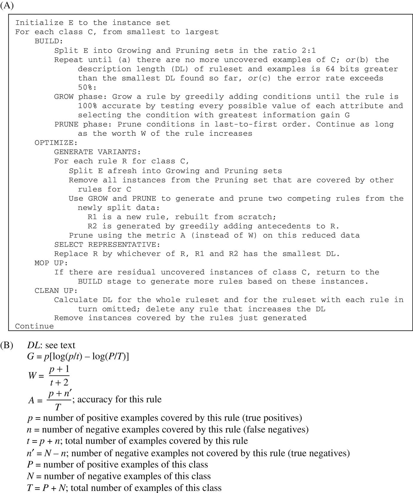
Suppose we split the training data into two parts that we will call a growing set and a pruning set. The growing set is used to form a rule using the basic covering algorithm. Then a test is deleted from the rule, and the effect is evaluated by trying out the truncated rule on the pruning set and seeing whether it performs better than the original rule. This pruning process repeats until the rule cannot be improved by deleting any further tests. The whole procedure is repeated for each class, obtaining one best rule for each class, and the overall best rule is established by evaluating the rules on the pruning set. This rule is then added to the rule set, the instances it covers removed from the training data—from both growing and pruning sets—and the process is repeated.
Why not do the pruning as we build the rule up, rather than building up the whole thing and then throwing parts away? That is, why not preprune rather than postprune? Just as when pruning decision trees it is often best to grow the tree to its maximum size and then prune back, so with rules it is often best to make a perfect rule and then prune it. Who knows?—adding that last term may make a really good rule, a situation that we might never have noticed had we adopted an aggressive prepruning strategy.
It is essential that the growing and pruning sets are separate, because it is misleading to evaluate a rule on the very data that was used to form it: that would lead to serious errors by preferring rules that were overfitted. Usually the training set is split so that two-thirds of instances are used for growing and one-third for pruning. A disadvantage, of course, is that learning occurs from instances in the growing set only, so the algorithm might miss important rules because some key instances had been assigned to the pruning set. Moreover, the wrong rule might be preferred because the pruning set contains only one-third of the data and may not be completely representative. These effects can be ameliorated by resplitting the training data into growing and pruning sets at each cycle of the algorithm, i.e., after each rule is finally chosen.
The idea of using a separate pruning set for pruning—which is applicable to decision trees as well as rule sets—is called reduced-error pruning. The variant described above prunes a rule immediately after it has been grown, and is called incremental reduced-error pruning. Another possibility is to build a full, unpruned, rule set first, pruning it afterwards by discarding individual tests. However, this method is much slower.
Of course, there are many different ways to assess the worth of a rule based on the pruning set. A simple measure is to consider how well the rule would do at discriminating the predicted class from other classes if it were the only rule in the rule set, operating under the closed world assumption. Suppose it gets p instances right out of the t instances that it covers, and there are P instances of this class out of a total T of instances altogether. The instances that it does not cover include N – n negative ones, where n=t – p is the number of negative instances that the rule covers and N=T – P is the total number of negative instances. Thus in total the rule makes correct decisions on p+(N – n) instances, and so has an overall success ratio of
This quantity, evaluated on the test set, has been used to evaluate the success of a rule when using reduced-error pruning.
This measure is open to criticism because it treats noncoverage of negative examples as equally important as coverage of positive ones, which is unrealistic in a situation where what is being evaluated is one rule that will eventually serve alongside many others. For example, a rule that gets p=2000 instances right out of a total coverage of 3000 (i.e., it gets n=1000 wrong) is judged as more successful than one that gets p=1000 out of a total coverage of 1001 (i.e., n=1 wrong), because [p+(N – n)]/T is [1000+N]/T in the first case but only [999+N]/T in the second. This is counterintuitive: the first rule is clearly less predictive than the second, because it has 33.3% as opposed to only 0.1% chance of being incorrect.
Using the success rate p/t as a measure, as was done in the original formulation of the covering algorithm (Fig. 4.8), is not the perfect solution either, because it will prefer a rule that gets a single instance right (p=1) out of a total coverage of 1 (so n=0) to the far more useful rule that gets 1000 right out of 1001. Another heuristic that has been used is (p – n)/t, but that suffers from exactly the same problem because (p – n)/t=2p/t – 1 and so the result, when comparing one rule with another, is just the same as with the success rate. It seems hard to find a simple measure of the worth of a rule that corresponds with intuition in all cases.
Whatever heuristic is used to measure the worth of a rule, the incremental reduced-error pruning algorithm is the same. A possible rule learning algorithm based on this idea is given in Fig. 6.3. It generates a decision list, creating rules for each class in turn and choosing at each stage the best version of the rule according to its worth on the pruning data. The basic covering algorithm for rule generation (Fig. 4.8) is used to come up with good rules for each class, choosing conditions to add to the rule using the accuracy measure p/t that we described earlier.

This method has been used to produce rule induction schemes that can process vast amounts of data and operate very quickly. It can be accelerated by generating rules for the classes in order rather than generating a rule for each class at every stage and choosing the best. A suitable ordering is the increasing order in which they occur in the training set so that the rarest class is processed first and the most common ones are processed later. Another significant speedup is obtained by stopping the whole process when a rule of sufficiently low accuracy is generated, so as not to spend time generating a lot of rules at the end with very small coverage. However, very simple terminating conditions (such as stopping when the accuracy for a rule is lower than the default accuracy for the class it predicts) do not give the best performance. One criterion that seems to work well is a rather complicated one based on the MDL principle, described below.
Using Global Optimization
In general, rules generated using incremental reduced-error pruning in this manner perform quite well, particularly on large datasets. However, it has been found that a worthwhile performance advantage can be obtained by performing a global optimization step on the set of rules induced. The motivation is to increase the accuracy of the rule set by revising or replacing individual rules. Experiments show that both the size and the performance of rule sets are significantly improved by postinduction optimization. On the other hand, the process itself is rather complex.
To give an idea of how elaborate industrial-strength rule learners become, Fig. 6.4 shows an algorithm called RIPPER, an acronym for repeated incremental pruning to produce error reduction. Classes are examined in increasing size and an initial set of rules for the class is generated using incremental reduced-error pruning. An extra stopping condition is introduced that depends on the description length (DL) of the examples and rule set. The description length DL is a complex formula that takes into account the number of bits needed to send a set of examples with respect to a set of rules, the number of bits required to send a rule with k conditions, and the number of bits needed to send the integer k—times an arbitrary factor of 50% to compensate for possible redundancy in the attributes. Having produced a rule set for the class, each rule is reconsidered and two variants produced, again using reduced-error pruning—but at this stage, instances covered by other rules for the class are removed from the pruning set, and success rate on the remaining instances is used as the pruning criterion. If one of the two variants yields a better DL, it replaces the rule. Next we reactivate the original building phase to mop up any newly uncovered instances of the class. A final check is made to ensure that each rule contributes to the reduction of DL, before proceeding to generate rules for the next class.
Obtaining Rules From Partial Decision Trees
There is an alternative approach to rule induction that avoids global optimization but nevertheless produces accurate and fairly compact rule sets. The method combines the divide-and-conquer strategy for decision tree learning with the separate-and-conquer one for rule learning. It adopts the separate-and-conquer strategy in that it builds a rule, removes the instances it covers, and continues creating rules recursively for the remaining instances until none are left. However, it differs from the standard approach in the way that each rule is created. In essence, to make a single rule, a pruned decision tree is built for the current set of instances, the leaf with the largest coverage is made into a rule, and the tree is discarded.
The prospect of repeatedly building decision trees only to discard most of them is not as bizarre as it first seems. Using a pruned tree to obtain a rule instead of pruning a rule incrementally by removing conjunctions one at a time avoids a tendency to overprune that is a characteristic problem of the basic separate-and-conquer rule learner. Using the separate-and-conquer methodology in conjunction with decision trees adds flexibility and speed. It is indeed wasteful to build a full decision tree just to obtain a single rule, but the process can be accelerated significantly without sacrificing the advantages.
The key idea is to build a partial decision tree instead of a fully explored one. A partial decision tree is an ordinary decision tree that contains branches to undefined subtrees. To generate such a tree, the construction and pruning operations are integrated in order to find a “stable” subtree that can be simplified no further. Once this subtree has been found, tree building ceases and a single rule is read off.
The tree-building algorithm is summarized in Fig. 6.5: it splits a set of instances recursively into a partial tree. The first step chooses a test and divides the instances into subsets accordingly. The choice is made using the same information-gain heuristic that is normally used for building decision trees (Section 4.3). Then the subsets are expanded in increasing order of their average entropy. The reason for this is that the later subsets will most likely not end up being expanded, and a subset with low average entropy is more likely to result in a small subtree and therefore produce a more general rule. This proceeds recursively until a subset is expanded into a leaf, and then continues further by backtracking. But as soon as an internal node appears that has all its children expanded into leaves, the algorithm checks whether that node is better replaced by a single leaf. This is just the standard subtree replacement operation of decision tree pruning (Section 6.1). If replacement is performed the algorithm backtracks in the standard way, exploring siblings of the newly replaced node. However, if during backtracking a node is encountered not all of whose children expanded so far are leaves—and this will happen as soon as a potential subtree replacement is not performed—then the remaining subsets are left unexplored and the corresponding subtrees are left undefined. Due to the recursive structure of the algorithm, this event automatically terminates tree generation.

Fig. 6.6 shows a step-by-step example. During the stages in Fig. 6.6A–C, tree building continues recursively in the normal way—except that at each point the lowest-entropy sibling is chosen for expansion: node 3 between stages (A) and (B). Gray elliptical nodes are as yet unexpanded; rectangular ones are leaves. Between stages (B) and (C), the rectangular node will have lower entropy than its sibling, node 5, but cannot be expanded further because it is a leaf. Backtracking occurs and node 5 is chosen for expansion. Once stage (C) is reached, there is a node—node 5—that has all its children expanded into leaves, and this triggers pruning. Subtree replacement for node 5 is considered and accepted, leading to stage (D). Now node 3 is considered for subtree replacement, and this operation is again accepted. Backtracking continues, and node 4, having lower entropy than node 2, is expanded into two leaves. Now subtree replacement is considered for node 4: suppose that node 4 is not replaced. At this point, the process terminates with the three-leaf partial tree of stage (E).

If the data is noise-free and contains enough instances to prevent the algorithm from doing any pruning, just one path of the full decision tree has to be explored. This achieves the greatest possible performance gain over the naïve method that builds a full decision tree each time. The gain decreases as more pruning takes place. For datasets with numeric attributes, the asymptotic time complexity of the algorithm is the same as building the full decision tree, because in this case the complexity is dominated by the time required to sort the attribute values in the first place.
Once a partial tree has been built, a single rule is extracted from it. Each leaf corresponds to a possible rule, and we seek the “best” leaf of those subtrees (typically a small minority) that have been expanded into leaves. Experiments show that it is best to aim at the most general rule by choosing the leaf that covers the greatest number of instances.
When a dataset contains missing values, they can be dealt with exactly as they are when building decision trees. If an instance cannot be assigned to any given branch because of a missing attribute value, it is assigned to each of the branches with a weight proportional to the number of training instances going down that branch, normalized by the total number of training instances with known values at the node. During testing, the same procedure is applied separately to each rule, thus associating a weight with the application of each rule to the test instance. That weight is deducted from the instance’s total weight before it is passed to the next rule in the list. Once the weight has reduced to zero, the predicted class probabilities are combined into a final classification according to the weights.
This yields a simple but surprisingly effective method for learning decision lists for noisy data. Its main advantage over other comprehensive rule-generation schemes is simplicity, because it does not require a complex global optimization stage.
Rules With Exceptions
In Section 3.4 we learned that a natural extension of rules is to allow them to have exceptions, and exceptions to the exceptions, and so on—indeed the whole rule set can be considered as exceptions to a default classification rule that is used when no other rules apply. The method of generating a “good” rule, using one of the measures described previously provides exactly the mechanism needed to generate rules with exceptions.
First, a default class is selected for the top-level rule: it is natural to use the class that occurs most frequently in the training data. Then, a rule is found pertaining to any class other than the default one. Of all such rules it is natural to seek the one with the most discriminatory power, e.g., the one with the best evaluation on a test set. Suppose this rule has the form
if <condition> then class = <new class>
It is used to split the training data into two subsets: one containing instances for which the rule’s condition is true and the other containing those for which it is false. If either subset contains instances of more than one class, the algorithm is invoked recursively on that subset. For the subset for which the condition is true, the “default class” is the new class as specified by the rule; for the subset where the condition is false, the default class remains as it was before.
Let’s examine how this algorithm would work for the rules with exceptions that were given in Section 3.4 for the iris data of Table 1.4. We will represent the rules in the graphical form shown in Fig. 6.7, which is in fact equivalent to the textual rules we showed before in Fig. 3.8. The default of Iris setosa is the entry node at the top left. Horizontal, dotted paths show exceptions, so the next box, which contains a rule that concludes Iris versicolor, is an exception to the default. Below this is an alternative, a second exception—alternatives are shown by vertical, solid lines—leading to the conclusion Iris virginica. Following the upper path along horizontally leads to an exception to the Iris versicolor rule that overrides it whenever the condition in the top right box holds, with the conclusion I. virginica. Below this is an alternative, leading (as it happens) to the same conclusion. Returning to the box at bottom center, this has its own exception, the lower right box, which gives the conclusion Iris versicolor. The numbers at the lower right of each box give the “coverage” of the rule, expressed as the number of examples that satisfy it divided by the number that satisfy its condition but not its conclusion. For example, the condition in the top center box applies to 52 of the examples, and 49 of them are Iris versicolor. The strength of this representation is that you can get a very good feeling for the effect of the rules from the boxes toward the left-hand side; the boxes at the right cover just a few exceptional cases.

To create these rules, the default is first set to I. setosa by taking the most frequently occurring class in the dataset. This is an arbitrary choice because for this dataset all classes occur exactly 50 times; as shown in Fig. 6.7 this default “rule” is correct in 50 out of 150 cases. Then the best rule that predicts another class is sought. In this case it is
if petal-length ≥ 2.45 and petal-length < 5.355 and petal-width < 1.75
then Iris-versicolor
This rule cover 52 instances, of which 49 are Iris versicolor. It divides the dataset into two subsets: the 52 instances that satisfy the condition of the rule and the remaining 98 that do not.
We work on the former subset first. The default class for these instances is Iris versicolor: there are only three exceptions, all of which happen to be I. virginica. The best rule for this subset that does not predict Iris versicolor is identified next:
if petal-length ≥ 4.95 and petal-width < 1.55 then Iris-virginica
It covers two of the three I. virginicas and nothing else. Again it divides the subset into two: those instances that satisfy its condition and those that do not. Fortunately, in this case, all those instances that satisfy the condition do indeed have class I. virginica, so there is no need for a further exception. However, the remaining instances still include the third I. virginica, along with 49 Iris versicolors, which are the default at this point. Again the best rule is sought:
if sepal-length < 4.95 and sepal-width ≥ 2.45 then Iris-virginica
This rule covers the remaining I. virginica and nothing else, so it also has no exceptions. Furthermore, all remaining instances in the subset that do not satisfy its condition have the class Iris versicolor, which is the default, so no more needs to be done.
Return now to the second subset created by the initial rule, the instances that do not satisfy the condition
petal-length ≥ 2.45 and petal-length < 5.355 and petal-width < 1.75
Of the rules for these instances that do not predict the default class I. setosa, the best is
if petal-length ≥ 3.35 then Iris-virginica
It covers all 47 Iris virginicas that are in the example set (3 were removed by the first rule, as explained previously). It also covers 1 Iris versicolor. This needs to be taken care of as an exception, by the final rule:
if petal-length < 4.85 and sepal-length < 5.95 then Iris-versicolor
Fortunately, the set of instances that do not satisfy its condition are all the default, I. setosa. Thus the procedure is finished.
The rules that are produced have the property that most of the examples are covered by the high-level rules and the lower-level ones really do represent exceptions. For example, the last exception clause and the deeply nested else clause both cover a solitary example, and removing them would have little effect. Even the remaining nested exception rule covers only two examples. Thus one can get an excellent feeling for what the rules do by ignoring all the deeper structure and looking only at the first level or two. That is the attraction of rules with exceptions.
Discussion
All algorithms for producing classification rules that we have describe use the basic covering or separate-and-conquer approach. For the simple, noise-free case this produces PRISM (Cendrowska, 1987), an algorithm that is simple and easy to understand. When applied to two-class problems with the closed world assumption, it is only necessary to produce rules for one class: then the rules are in disjunctive normal form and can be executed on test instances without any ambiguity arising. When applied to multiclass problems, a separate rule set is produced for each class: thus a test instance may be assigned to more than one class, or to no class, and further heuristics are necessary if a unique prediction is sought.
To reduce overfitting in noisy situations, it is necessary to produce rules that are not “perfect” even on the training set. To do this it is necessary to have a measure for the “goodness,” or worth, of a rule. With such a measure it is then possible to abandon the class-by-class approach of the basic covering algorithm and start by generating the very best rule, regardless of which class it predicts, and then remove all examples covered by this rule and continue the process. This yields a method for producing a decision list rather than a set of independent classification rules, and decision lists have the important advantage that they do not generate ambiguities when interpreted.
The idea of incremental reduced-error pruning is due to Fürnkranz and Widmer (1994) and forms the basis for fast and effective rule induction. The RIPPER rule learner is due to Cohen (1995), although the published description appears to differ from the implementation in precisely how the DL affects the stopping condition. What we have presented here is the basic idea of the algorithm; there are many more details in the implementation.
The whole question of measuring the value of a rule is a difficult one. Many different measures have been proposed, some blatantly heuristic and others based on information-theoretical or probabilistic grounds. However, there seems to be no consensus on what the best measure to use is. An extensive theoretical study of various criteria has been performed by Fürnkranz and Flach (2005).
The rule learning scheme based on partial decision trees was developed by Frank and Witten (1998). On standard benchmark datasets it produces rule sets that are as accurate as rules generated by the C4.5 rule learner, and often more accurate than those of RIPPER; however, it produces larger rule sets than RIPPER. Its main advantage over other schemes is not performance but simplicity: by combining top-down decision tree induction with separate-and-conquer rule learning, it produces good rule sets without any need for global optimization.
The procedure for generating rules with exceptions was developed as an option in the Induct system by Gaines and Compton (1995), who called them ripple-down rules. In an experiment with a large medical dataset (22,000 instances, 32 attributes, and 60 classes), they found that people can understand large systems of rules with exceptions more readily than equivalent systems of regular rules because that is the way that they think about the complex medical diagnoses that are involved. Richards and Compton (1998) describe their role as an alternative to classic knowledge engineering.
6.3 Association Rules
In Section 4.5 we studied the Apriori algorithm for generating association rules that meet minimum support and confidence thresholds. Apriori follows a generate-and-test methodology for finding frequent item sets, generating successively longer candidate item sets from shorter ones that are known to be frequent. Each different size of candidate item set requires a scan through the dataset in order to determine whether its frequency exceeds the minimum support threshold. Although some improvements to the algorithm have been suggested to reduce the number of scans of the dataset, the combinatorial nature of this generation process can prove costly—particularly if there are many item sets or item sets are large. Both these conditions readily occur even for modest datasets when low support thresholds are used. Moreover, no matter how high the threshold, if the data is too large to fit in main memory it is undesirable to have to scan it repeatedly—and many association rule applications involve truly massive datasets.
These effects can be ameliorated by using appropriate data structures. We describe a method called FP-growth that uses an extended prefix tree—a frequent pattern tree or “FP-tree”—to store a compressed version of the dataset in main memory. Only two passes are needed to map a dataset into an FP-tree. The algorithm then processes the tree in a recursive fashion to grow large item sets directly, instead of generating candidate item sets and then having to test them against the entire database.
Building a Frequent Pattern Tree
Like Apriori, the FP-growth algorithm begins by counting the number of times individual items (i.e., attribute–value pairs) occur in the dataset. After this initial pass, a tree structure is created in a second pass. Initially the tree is empty and the structure emerges as each instance in the dataset is inserted into it.
The key to obtaining a compact tree structure that can be quickly processed to find large item sets is to sort the items in each instance in descending order of their frequency of occurrence in the dataset, which has already been recorded in the first pass, before inserting them into the tree. Individual items in each instance that do not meet the minimum support threshold are not inserted into the tree, effectively removing them from the dataset. The hope is that many instances will share those items that occur most frequently individually, resulting in a high degree of compression close to the tree’s root.
We illustrate the process with the weather data, reproduced in Table 6.1A, using a minimum support threshold of 6. The algorithm is complex, and its complexity far exceeds what would be reasonable for such a trivial example, but a small illustration is the best way of explaining it. Table 6.1B shows the individual items, with their frequencies, that are collected in the first pass. They are sorted into descending order and ones whose frequency exceeds the minimum threshold are in bold. Table 6.1C shows the original instances, numbered as in Table 6.1A, with the items in each instance sorted into descending frequency order. Finally, to give an advance peek at the final outcome, Table 6.1D shows the only two multiple-item sets whose frequency satisfies the minimum support threshold. Along with the six single-item sets shown in bold in Table 6.1B, these form the final answer: a total of eight item sets. We are going to have to do a lot of work to find the two multiple-item sets in Table 6.1D using the FP-tree method.
Table 6.1
Preparing the Weather Data for Insertion Into an FP-tree: (A) The Original Data; (B) Frequency Ordering of Items With Frequent Item Sets in Bold; (C) The Data With Each Instance Sorted Into Frequency Order; (D) The Two Multiple-Item Frequent Item Sets
| Outlook | Temperature | Humidity | Windy | Play | ||
| (A) | 1 | Sunny | Hot | High | False | No |
| 2 | Sunny | Hot | High | True | No | |
| 3 | Overcast | Hot | High | False | Yes | |
| 4 | Rainy | Mild | High | False | Yes | |
| 5 | Rainy | Cool | Normal | False | Yes | |
| 6 | Rainy | Cool | Normal | True | No | |
| 7 | Overcast | Cool | Normal | True | Yes | |
| 8 | Sunny | Mild | High | False | No | |
| 9 | Sunny | Cool | Normal | False | Yes | |
| 10 | Rainy | Mild | Normal | False | Yes | |
| 11 | Sunny | Mild | Normal | True | Yes | |
| 12 | Overcast | Mild | High | True | Yes | |
| 13 | Overcast | Hot | Normal | False | Yes | |
| 14 | Rainy | Mild | High | True | No |
| (B) | Play=yes | 9 |
| Windy=false | 8 | |
| Humidity=normal | 7 | |
| Humidity=high | 7 | |
| Windy=true | 6 | |
| Temperature=mild | 6 | |
| Play=no | 5 | |
| Outlook=sunny | 5 | |
| Outlook=rainy | 5 | |
| Temperature=hot | 4 | |
| Temperature=cool | 4 | |
| Outlook=overcast | 4 |
| (C) | 1 | Windy=false, humidity=high, play=no, outlook=sunny, temperature=hot |
| 2 | Humidity=high, windy=true, play=no, outlook=sunny, temperature=hot | |
| 3 | Play=yes, windy=false, humidity=high, temperature=hot, outlook=overcast | |
| 4 | Play=yes, windy=false, humidity=high, temperature=mild, outlook=rainy | |
| 5 | Play=yes, windy=false, humidity=normal, outlook=rainy, temperature=cool | |
| 6 | Humidity=normal, windy=true, play=no, outlook=rainy, temperature=cool | |
| 7 | Play=yes, humidity=normal, windy=true, temperature=cool, outlook=overcast | |
| 8 | Windy=false, humidity=high, temperature=mild, play=no, outlook=sunny | |
| 9 | Play=yes, windy=false, humidity=normal, outlook=sunny, temperature=cool | |
| 10 | Play=yes, windy=false, humidity=normal, temperature=mild, outlook=rainy | |
| 11 | Play=yes, humidity=normal, windy=true, temperature=mild, outlook=sunny | |
| 12 | Play=yes, humidity=high, windy=true, temperature=mild, outlook=overcast | |
| 13 | Play=yes, windy=false, humidity=normal, temperature=hot, outlook=overcast | |
| 14 | Humidity=high, windy=true, temperature=mild, play=no, outlook=rainy |
| (D) | Play=yes & windy=false | 6 |
| Play=yes & humidity=normal | 6 |

Fig. 6.8A shows the FP-tree structure that results from this data with a minimum support threshold of 6. The tree itself is shown with solid arrows. The numbers at each node show how many times the sorted prefix of items, up to and including the item at that node, occur in the dataset. For example, following the third branch from the left in the tree we can see that, after sorting, two instances begin with the prefix humidity=high—the second and last instances of Table 6.1C. Continuing down that branch, the next node records that the same two instances also have windy=true as their next most frequent item. The lowest node in the branch shows that one of these two instances (the last in Table 6.1C) contain temperature=mild as well. The other instance (the second in the Table) drops out at this stage because its next most frequent item does not meet the minimum support constraint and is therefore omitted from the tree.


On the left-hand side of the diagram a “header table” shows the frequencies of the individual items in the dataset (Table 6.1B). These items appear in descending frequency order, and only those with at least minimum support are included. Each item in the header table points to its first occurrence in the tree, and subsequent items in the tree with the same name are linked together to form a list. These lists, emanating from the header table, are shown in Fig. 6.8A by dashed arrows.
It is apparent from the tree that only two nodes have counts that satisfy the minimum support threshold, corresponding to the item sets play=yes (count of 9) and play=yes & windy=false (count of 6) in the leftmost branch. Each entry in the header table is itself a single-item set that also satisfies the threshold. This identifies as part of the final answer all the bold items in Table 6.1B and the first item set in Table 6.1D. Since we know the outcome in advance we can see that there is only one more item set to go—the second in Table 6.1D. But there is no hint of it in the data structure of Fig. 6.8A, and we will have to do a lot of work to discover it!
Finding Large Item Sets
The purpose of the links from the header table into the tree structure is to facilitate traversal of the tree to find other large item sets, apart from the two that are already in the tree. This is accomplished by a divide-and-conquer approach that recursively processes the tree to grow large item sets. Each header table list is followed in turn, starting from the bottom of the table and working upwards. Actually, the header table can be processed in any order, but it is easier to think about processing the longest paths in the tree first, and these correspond to the lower-frequency items.
Starting from the bottom of the header table, we can immediately add temperature=mild to the list of large item sets. Fig. 6.8B shows the result of the next stage, which is an FP-tree for just those instances in the dataset that include temperature=mild. This tree was not created by rescanning the dataset but by further processing of the tree in Fig. 6.8A, as follows.
To see if a larger item set containing temperature=mild can be grown, we follow its link from the header table. This allows us to find all instances that contain temperature=mild. From here the new tree in Fig. 6.8B is created, with counts projected from the original tree corresponding to the set of instances that are conditional on the presence of temperature=mild. This is done by propagating the counts from the temperature=mild nodes up the tree, each node receiving the sum of its children’s counts.
A quick glance at the header table for this new FP-tree shows that the temperature=mild pattern cannot be grown any larger because there are no individual items, conditional on temperature=mild, that meet the minimum support threshold. Note, however, that it is necessary to create the whole Fig. 6.8B tree in order to discover this, because it is effectively being created bottom up and the counts in the header table to the left are computed from the numbers in the tree. The recursion exits at this point, and processing continues on the remaining header table items in the original FP-tree.
Fig. 6.8C shows a second example, the FP-tree that results from following the header table link for humidity=normal. Here the windy=false node has a count of 4, corresponding to the four instances that had humidity=normal in its left branch in the original tree. Similarly, play=yes has a count of 6, corresponding to the four instances from windy=false and the two instances that contain humidity=normal from the middle branch of the subtree rooted at play=yes in Fig. 6.8A.
Processing the header list for this FP-tree shows that the humidity=normal item set can be grown to include play=yes since these two occur together six times, which meets the minimum support constraint. This corresponds to the second item set in Table 6.1D, which in fact completes the output. However, in order to be sure that there are no other eligible item sets it is necessary to continue processing the entire header link table in Fig. 6.8A.
Once the recursive tree mining process is complete all large item sets that meet the minimum support threshold have been found. Then association rules are created using the approach explained in Section 4.5. Studies have claimed that the FP-growth algorithm is up to an order of magnitude faster than Apriori at finding large item sets, although this depends on the details of the implementation and the nature of the dataset.
Discussion
The process of recursively creating projected FP-trees can be efficiently implemented within a single prefix tree structure by having a list of frequencies, indexed by recursion depth, at each node in the tree and each element of the header table. The tree structure itself is usually far smaller than the original dataset, and if the dataset is dense it achieves a high level of compression. This outweighs the overhead imposed by the pointers and counters that must be maintained at each node. Only when the support threshold is set very low does the FP-tree’s ability to compress the dataset degrade. Under these conditions, the tree becomes bushy, with little node sharing. On massive datasets for which the FP-tree exceeds main memory, disk-resident trees can be constructed using indexing techniques that have been developed for relational database systems.
The FP-tree data structure and FP-growth algorithm for finding large item sets without candidate generation were introduced by Han, Pei, and Yin (2000) following pioneering work by Zaki, Parthasarathy, Ogihara, and Li (1997); Han, Pei, Yin, and Mao (2004) give a more comprehensive description. It has been extended in various ways. Wang, Han, and Pei (2003) develop an algorithm called CLOSET+ to mine closed item sets, i.e., sets for which there is no proper superset that has the same support. Finding large closed item sets provides essentially the same information as finding the complete set of large item sets, but produces few redundant rules and thus eases the task that users face when examining the output of the mining process. GSP, for Generalized Sequential Patterns, is a method based on the Apriori algorithm for mining patterns in databases of event sequences (Srikant & Agrawal, 1996). A similar approach to FP-growth is used for event sequences by algorithms called PrefixSpan (Pei et al., 2004) and CloSpan (Yan, Han, & Afshar, 2003), and for graph patterns by algorithms called gSpan (Yan & Han, 2002) and CloseGraph (Yan & Han, 2003).
Ceglar and Roddick (2006) provide a comprehensive survey of association rule mining. Some authors have worked on integrating association rule mining with classification. For example, Liu, Hsu, and Ma (1998) mine a kind of association rule that they call a “class association rule,” and build a classifier on the rules that are found using a technique they call CBA. Mutter, Hall, and Frank (2004) use classification to evaluate the output of confidence-based association rule mining, and find that standard learners for classification rules are generally preferable to CBA when run time and size of the rule sets is of concern.
6.4 Weka Implementations
SimpleCart (minimum cost-complexity pruning à la CART, in the simpleCART package)
REPTree (reduced-error pruning)
Part (rules from partial decision trees)
Ridor (ripple-down rule learner, in the ridor package)
FPGrowth (frequent pattern trees).
GeneralizedSequentialPatterns (find large item trees in sequential data, in the generalizedSequentialPatterns package)
CBA (mining class association rules, in the classAssociationRules package)