3.1 Random variables

Every practitioner of data analysis needs a working knowledge of probability for one simple reason: error, an unavoidable aspect of measurement, is best understood using the ideas of probability.

The key concept that we draw upon is the random variable. If d is a random variable, then it has no fixed value until it is realized. Think of d as being in a box. As long as it is in the box, its value is fuzzy or indeterminate; but when taken out of the box and examined, d takes on a specific value. It has been realized. Put it back in the box, and its value becomes indeterminate again. Take d out again and it will have a different value, as it is now a different realization. This behavior is analogous to measurement in the presence of noise, so random variables are ideal for representing noisy data.

Even when the random variable, d, is in the box, we may know something about it. It may have a tendency to take on certain values more often than others. For example, suppose that d represents the number of H (hydrogen) atoms in a CH₄ (methane) molecule that are of the heavy variety called deuterium. Then d can take on only the discrete values 0 through 4, with d = 0 representing the no deuterium state and d = 4 representing the all deuterium state. The tendency of d to take on one of these five values is represented by its probability, P(d), which can be depicted by a table (Figure 3.1A).

Note that the probability is given in percent, that is, the percent of the realizations in which d takes on the given value. The probability necessarily sums to 100%, as d must take on one of the five possible values. We can write${\sum }_{i=0}^{4}P(d_i)=100\%$. An alternative way of quantifying probability is with the numbers 0-1, with 0 meaning 0% and 1 meaning 100% (Figure 3.1B). In this case, ${\sum }_{i=0}^{4}P(d_i)=1$. The probability can also be represented graphically with a histogram (Figure 3.1C) or a shaded column vector (Figure 3.1D).

Not all random variables are discrete. Some may vary continuously between two extremes. Thus, for example, the depth, d, of a fish observed swimming in a 5-m-deep pond can take on any value, even fractional ones, between 0 and 5. In this continuous case, we quantify the probability that the fish is near depth, d, with the probability density function, p(d). The probability, P, that the fish is observed between any two depths, say d₁ and d₂, is defined as the area under the curve p(d) between d₁ and d₂ (Figure 3.2). This is equivalent to the integral

$P(d_1,d_2)={\int }_{d_1}^{d_2}p\left(d\right)\text{d}d$

(Our choice of the variable name “d” for “data” makes the differential dd look a bit funny, but we will just have to live with it!) Note the distinction between upper-case and lower-case letters. Upper-case P, which quantifies probability, is a number between 0 and 1. Lower-case p is a function whose values are not easily interpretable, except to the extent that the larger the p, the more likely that a realization will have a value near d. One must calculate the area, which is to say, perform the integral, to determine how likely any given range of d is. Just as in the discrete case, d must take on some value between its minimum and maximum (in this case, d_min = 0 and d_max = 5). Thus

$P(d_{\text{min}},d_{\text{max}})={\int }_{d_{\text{min}}}^{d_{\text{max}}}p\left(d\right)\text{d}d=1$

The function, P(d_min, d) (or P(d), for short), which gives the total amount of probability less than d, is called the probability distribution (or, sometimes, the cumulative probability distribution) of the random variable, d.

Because all measurements contain noise, we view every measurement, d, as a random variable. Several repetitions of the same measurement will not necessarily yield the same value because of measurement error. On the other hand, repeated measurements usually have some sort of systematic behavior, such as scattering around a typical value. This systematic behavior will be represented by the probability density function, p(d). Thus, p(d) embodies both the “true” value of the quantity (if such a thing can be said to exist) and a description of the measurement noise.

Practitioners of data analysis very typically compute derived quantities from their data that are more relevant to the objective of their study. For example, temperature measurements made at different times might be differenced (subtracted) in order to determine a rate of warming. As we will discuss further below, functions of random variables are themselves random variables, because any quantity derived from noisy data itself contains error. The algebra of random variables will allow us to understand how measurement noise affects inferences made from the data.

3.2 Mean, median, and mode

The probability density function of a measurement, p(d), is a function—possibly one with a complicated shape. As an aid to understanding it, one might try to derive from it two simple numbers, one that describes the typical measurement (i.e., the typical d) and the other which describes the variability of measurements (i.e., the amount of scatter around the typical measurement). Of course, the two numbers cannot completely capture the information in p(d), but they can provide some insight into its behavior.

Several different approaches to calculating a typical value of d are in use. The simplest is the d at which p(d) takes on its maximum value, which is called the maximum likelihood point or mode. The mode is useful because, in a list of repeated measurements, a particular value is often seen to occur more frequently than any other value. Modes can be deceptive, however, because while more measurements will be in the vicinity of the mode than in the vicinity of any other value of d, the majority of measurements are not necessarily in the vicinity of the mode. This effect is illustrated in Figure 3.3, which depicts a very skewed probability density function, p(d) and a corresponding table of binned data. More data—15—are observed in the 1 < d < 2 bin, which encloses the mode, than in any other bin. Nevertheless, full 80% of the measurements are larger than the mode, and 50% are quite far from it.

This effect is often encountered in real-world situations. Thus, for example, while ironwood (Memecylon umbellatum) is by far the most common of the ~50 species of trees in the evergreen forests of India's Eastern Ghats, a randomly chosen tree there would most likely not be ironwood, as this species accounts for only 21% of the individual trees (Chittibabu and Parthasarathy, 2000).

In MatLab, suppose that the column-vector, d, is d sampled at evenly spaced points, and that the column-vector, p, contains the corresponding values of p(d). Then the mode is calculated as follows:

[pmax, i] = max(p);
themode = d(i);

(MatLab eda03_01)

Note that the function, max(p), returns both the maximum value, pmax, of the column-vector, p, and the row index, i, at which the maximum value occurs.

Another way of defining the typical measurement is to pick the value below which 50% of probability falls and above which lies the other 50%. This quantity is called the median (Figure 3.4).

In MatLab, suppose that the column vector d contains the data d sampled at evenly spaced points, with spacing Dd, and that the column vector p contains the corresponding values of p(d). Then, the median is calculated as follows:

pc = Dd*cumsum(p);
for i=[1:length(p)]
 if(pc(i) > 0.5 )
 themedian = d(i);
 break;
 end
end

(MatLab eda03_02)

The function cumsum() computes the cumulative sum (running sum) of p. The quantity, Dd*cumsum(p), is thus an approximation for the indefinite integral, ${\int }_{d_{\text{min}}}^{d}p(d)\text{d}d$, which is to say the area beneath p(d). The for loop then searches for the first occurrence of the area that is greater than 0.5, terminating (“breaking”) when this condition is satisfied.

Yet another common way to define a typical value is a generalization of the mean value of a set of measurements. The well-known formula for the sample mean is $\overline{d}=1/N{\sum }_{i=0}^N{d}_i$. Let's approximate this formula with a histogram. First, divide the d-axis into M small bins, each one centered at d^(s). Now count up the number, N_s, of data in each bin. Then, $\overline{d}\approx 1/N{\sum }_{s=0}^M{d}^{(s)}{N}_s$. Note that the quantity N_s/N is the frequency of d_i; that is, the fraction of times that d_i is observed to fall in bin s. As this frequency is, approximately, the probability, P_s, that the data falls in bin s, $\overline{d}\approx {{\sum }_{s=0}^M{d}^{(s)}P}_s$. This relationship suggests that the mean of the probability density function, p(d), can be defined as

$\overline{d}={\int }_{d_{\text{min}}}^{d_{\text{max}}}dp(d)\text{d}d$

Because of random variation, the mean of a set of measurements (the sample mean) will not be the same as the mean of the probability density function from which the measurements were drawn. However, as we will discuss later in this book, the sample mean will usually be close to—will scatter around—the mean of the probability density function (Figure 3.5).

In MatLab, suppose that the column-vector, d, contains the d sampled at evenly spaced points, with spacing Dd, and that the column-vector, p, contains the corresponding values of p(d). The definite integral${\int }_{d_{\text{min}}}^{d}dp(d)\text{d}d$ is approximated as ${\sum }_i{d}_{i}p(d_i)\Delta d$ as follows:

themean = Dd*sum(d.*p);

(MatLab eda03_03)

Note that the sum(v) function returns the sum of the elements of the column-vector, v.

3.3 Variance

The second part of the agenda that we put forward in Section 3.2 is to devise a number that describes the amount of scatter of the data around its typical value. This number should be large for a wide probability density function—one that corresponds to noisy measurements—and small for a narrow one. A very intuitive choice for a measure of the width of a probability density function, p(d), is the length, d₅₀, of the d-axis that encloses 50% of the total probability and is centered around the typical value, d_typical. (This quantity is called the interquartile). Then, 50% of measurements would scatter between d_typical − d₅₀/2 and d_typical + d₅₀/2 (Figure 3.6). Probability density functions with a large d₅₀ correspond to a high-noise measurement scenario and probability density functions with a small d₅₀ correspond to a low-noise one. Unfortunately, this definition is only rarely used in the literature.

A much more commonly encountered—but much less intuitive—quantity is the variance. It is based on a different approach to quantifying width, one not directly related to probability. Consider the quadratic function q(d) = (d − d_typical)². It is small near d_typical and large far from it. The product, q(d) p(d), will be small everywhere if the probability density function is narrow, as near d_typical, large values of p(d) will be offset by small values of q(d) and far from d_typical, large values of q(d) will be offset by small values of p(d). The area under the product, q(d) p(d), will be small in this case. Conversely, the area under the product, q(d) p(d), will be large if the probability density function is wide. Thus, the area under q(p) p(d) has the desired property of being small for narrow probability density functions and large for wide ones (Figure 3.7). With the special choice, $d_{\text{typical}}=\overline{d}$, it is called the variance and is given the symbol, σ_d²:

${\sigma }_d^2={\int }_{d_{\text{min}}}^{d_{\text{max}}}{(d-\overline{d})}^{2}p(d)\text{d}d$

Variance has units of d², so the square root of variance, σ, is a measure of the width of the probability density function. A disadvantage of the variance is that the relationship between it and the probability that $\overline{d}\pm \sigma$ encloses is not immediately known. It depends on the functional form of the probability density function.

In MatLab, suppose that the column-vector, d, contains the data, d, sampled at evenly spaced points, with spacing Dd and that the column-vector, p, contains the corresponding values of p(d). Then, the variance, σ², is calculated as follows:

q = (d−dbar).○2;
sigma2 = Dd*sum(q.*p);
sigma = sqrt(sigma2);

(MatLab eda03_04)

3.4 Two important probability density functions

As both natural phenomena and the techniques that we use to observe them are greatly varied, it should come as no surprise that hundreds of different probability density functions, each with its own mathematical formula, have been put forward as good ways to model particular classes of noisy observations. Yet among these, two particular probability density functions stand out in their usefulness.

The first is the uniform probability density function, p(d) = constant. This probability density function could be applied in the case of a measurement technique that can detect a fish in a lake, but which provides no information about its depth, d. As far as can be determined, the fish could be at any depth with equal probability, from its surface, d = d_min, to its bottom, d = d_max. Thus, the uniform probability density function is a good idealization of the limiting case of a measurement providing no useful information. The uniform probability density function is properly normalized when the constant is 1/(d_max − d_min), where the data range from d_min to d_max. Note that the uniform probability density function can be defined only when the range is finite. It is not possible for data to be anything in the range from −∞ to +∞ with equal probability.

The second is the Normal probability density function:

$p(d)=\frac{1}{\sqrt{2\pi }\sigma }exp\left\{-\frac{{(d-\overline{d})}^2}{2{\sigma }^2}\right\}$

The constants have been chosen so that the probability density function, when integrated over the range −∞ < d < +∞, has unit area and so that its mean is $\overline{d}$ and its variance is σ². Not only is the Normal curve centered at the mean, but it is peaked at the mean and symmetric about the mean (Figure 3.8). Thus, both its mode and median are equal to its mean, $\overline{d}$. The probability, P, enclosed by the interval $\overline{d}\pm n\sigma$ (where n is an integer) is given by the following table:

$\begin{array}{ll}n\hfill & P,\%\hfill \\ 1\hfill & 68.27\hfill \\ 2\hfill & 95.45\hfill \\ 3\hfill & 99.73\hfill \end{array}$

It is easy to see why the Normal probability density function is seen as an attractive one with which to model noisy observations. The typical observation will be near its mean, $\overline{d}$, which is equal to the mode and median. Most of the probability (99.73%) is concentrated within ±3σ of the mean and only very little probability (0.27%) lies outside that range. Because of the symmetry, the behavior of measurements less than the mean is the same as the behavior greater than the mean. Many measurement scenarios behave just in this way.

On the other hand, the Normal probability density function does have limitations. One limitation is that it is defined on the unbounded interval −∞ < d < +∞, while in many instances data are bounded. The fish in the pond example, discussed above, is one of these. Any Normal probability density function, regardless of mean and variance, predicts some probability that the fish will be observed either in the air or buried beneath the bottom of the pond, which is unrealistic. Another limitation arises from the rapid falloff of probability away from the mean—behavior touted as good in the previous paragraph. However, some measurement scenarios are plagued by outliers, occasional measurements that are far from the mean. Normal probability density functions tend to under-predict the frequency of outliers.

While not all noise processes are Normally distributed, the Normal probability density function occurs in a wide range of situations. Its ubiquity is understood to be a consequence a mathematical result of probability theory called the Central Limit Theorem: under a fairly broad range of conditions, the sum of a sufficiently large number of random variables will be approximately Normally distributed, regardless of the probability density functions of the individual variables. Measurement error often arises from a several different sources of noise, which sum together to produce the overall error. The Central Limit Theorem predicts that, in this case, the overall error will be Normally distributed even when the component sources are not.

3.5 Functions of a random variable

An important aspect of data analysis is making inferences from data. The making of measurements is not an end unto itself, but rather the observations are used to make specific, quantitative predictions about the world. This process often consists of combining the data into a smaller number of more meaningful model parameters. These derived parameters are therefore functions of the data.

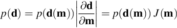
The simplest case is a model parameter, m, that is a function of a single random variable, d; that is, m = m(d). We need a method of determining the probability density function, p(m), given the probability density function, p(d), together with the functional relationship, m(d). The appropriate rule can be found by starting with the formula relating the probability density function, p(d), to the probability, P, (Equation 3.1) and applying the chain rule.

$P(d_1,d_2)={\int }_{d_1}^{d_2}p(d)\text{d}d={\int }_{d_1(m_1)}^{d_2(m_2)}p[d(m)]\frac{\partial d}{\partial m}\text{d}m={\int }_{m_1}^{m_2}P(m)dm=P(m_1,m_2)$

where (m₁, m₂) corresponds to (d₁, d₂); that is m₁ = m(d₁) and m₂ = m(d₂). Then by inspection, $p(m)=p[d(m)]\partial d/\partial m$. In some cases, such as the function m(d) = 1/d, the derivative $\partial d/\partial m$ is negative, corresponding to the situation where m₁ > m₂ and the direction of integration along the m-axis is reversed. To account for this case, we take the absolute value of $\partial d/\partial m$:

$p(m)=p[d(m)]\left|\frac{\partial d}{\partial m}\right|$

with the understanding that the integration is always performed from the smaller of (m₁, m₂) to the larger.

The significance of the $\partial d/\partial m$ factor can be understood by considering the uniform probability density function P(d) = 1 on the interval 0 ≤ d ≤ 1 together with the function m = 2d. The interval 0 ≤ d ≤ 1 corresponds to the interval 0 ≤ m ≤ 2 and $\partial d/\partial m=½$. Equation (3.8) gives p(m) = 1 × ½ = ½, that is p(m) is also a uniform probability density function, but with a different normalization than p(d). The total area, A, beneath both p(d) and p(m) is the same, A = 1 × 1 = 2 × ½ = 1. Thus, $\partial d/\partial m$ acts as a scale factor that accounts for the way that the stretching or squeezing of the m-axis relative to the d-axis affects the calculation of area.

As linear functions, such as m = cd, where c is a constant, are common in data analysis, we mention one of their important properties here. Suppose that p(d) has mean, $\overline{d}$, and variance, ${\sigma }_d^2$. Then, the mean, $\overline{m}$, and variance, ${\sigma }_m^2$, of p(m) are as follows:

$\overline{m}=\int mp\left(m\right)\text{d}m=\int cdp[d\left(m\right)]\frac{\partial d}{\partial m}\frac{\partial m}{\partial d}\text{d}d=c\int dp(d)\text{d}d=c\overline{d}$

${\sigma }_m^2=\int {(m-\overline{m})}^{2}p(m)\text{d}m=\int {(cd-c\overline{d})}^{2}p[d(m)]\frac{\partial d}{\partial m}\frac{\partial m}{\partial d}\text{d}d=c^2\int {(d-\overline{d})}^{2}p(d)\text{d}d=c^2{\sigma }_d^2$

Thus, in the special case of the linear function, m = cd, the formulas

$\overline{m}=c\overline{d}\text{and}{\sigma }_m^2=c^2{\sigma }_d^2$

do not depend on the functional form of the probability density function, p(d).

In another example of computing the probability density function of a function of a random variable, consider the probability density function p(d) = 1 on the interval 0 ≤ d ≤ 1 and the function, m = d². The corresponding interval of m is 0 ≤ d ≤ 1, d = m^½, and $\partial d/\partial m=½m^{-½}$. The probability density function, p(m), is given as

$p(m)=p[d(m)]\frac{\partial d}{\partial m}=1\times ½m^{-½}=½m^{-½}$

on the interval 0 ≤ m ≤ 1. Unlike p(d), the probability density function p(m) is not uniform but rather has a peak (actually a singularity, but an integrable one) at m = 0 (Figure 3.9).

In this section, we have described how the probability density function of a function of a single observation, d, can be computed. For this technique to be truly useful, we must generalize it so that we can compute the probability density function of a function of a set of many observations. However, before tackling this problem, we will need to discuss how to describe the probability density function of a set of observations.

3.6 Joint probabilities

Consider the following scenario: A certain island is inhabited by two species of birds, gulls and pigeons. Either species can be either tan or white in color. A census determines that 100 birds live on the island, 30 tan pigeons, 20 white pigeons, 10 tan gulls and 40 white gulls. Now suppose that we visit the island. The probability of sighting a bird of species, s, and color, c, can be summarized by a 2 × 2 table (Figure 3.10), which is called the joint probability of species, s, and color, c, and is denoted by P(s, c). Note that the elements of the table must sum to 100%: ${\sum }_{i=1}^2{\sum }_{j=1}^{2}P(s_i,c_j)=100\%$. P(s, c) completely describes the situation, and other probabilities can be calculated from it. If we sum the elements of each row, we obtain the probability that the bird is a given species, irrespective of its color: $P(s)={\sum }_{j=1}^{2}P(s,c_j)$. Likewise, if we sum the elements of each column, we obtain the probability that the bird is a given color, irrespective of its species: $P(c)={\sum }_{i=1}^{2}P(s_i,c)$ (Figure 3.11).

Suppose that we observe the color of a bird but are not able to identify its species. Given that its color is c, what is the probability that it is of species s ? This is called the conditional probability of s given c and is written as P(s|c). We compute it by dividing every element of P(s, c) by the total number of birds of that color (Figure 3.12):

$P(s|c)=\frac{P(s,c)}{{\sum }_{i=1}^{2}P(s_i,c)}=\frac{P(s,c)}{P(c)}$

Alternatively, we could ask, given that its species is s, what is the probability that it is of color c? This is the conditional probability of c given s, and is written as P(c|s). We compute it by dividing every element of P(s, c) by the total amount of birds of that species:

$P(c|s)=\frac{P(s,c)}{{\sum }_{j=1}^{2}P(s,c_j)}=\frac{P(s,c)}{P(s)}$

Equations (3.13) and (3.14) can be combined to give a very important result called Bayes Theorem:

$P(s,c)=P(s|c)P(c)=P(c|s)P(s)$

Bayes Theorem can also be written as

$\begin{array}{c}P(s|c)=\frac{P(c|s)P(s)}{P(c)}=\frac{P(c|s)P(s)}{{\sum }_{i}P(s_i,c)}=\frac{P(c|s)P(s)}{{\sum }_{i}P(c|s_i)P(s_i)}\\ P(c|s)=\frac{P(s|c)P(c)}{P(s)}=\frac{P(s|c)P(c)}{{\sum }_{j}P(s,c_j)}=\frac{P(s|c)P(c)}{{\sum }_{j}P(s|c_j)P(c_j)}\end{array}$

Note that we have used the following relations:

$\begin{array}{c}P(c)={\sum }_{i}P(s_i,c)={\sum }_{i}P(c|s_i)P(s_i)\\ P(s)={\mathbf{\sum }}_{j}P(s,c_j)={\sum }_{j}P(s|c_j)P(c_j)\end{array}$

Note that the two conditional probabilities are not equal; that is, P(s|c)≠P(c|s). Confusion between the two is a major source of error in both scientific and popular circles! For example, the probability that a person who contracts pancreatic cancer “C” will die “D” from it is very high, P(D|C) ≈ 90%. In contrast, the probability that a dead person succumbed to pancreatic cancer, as contrasted to some other cause of death, is much lower, P(C|D) ≈ 1.4%. Yet, the news of a person dying of pancreatic cancer usually provokes more fear among people who have no reason to suspect that they have the disease than this low probability warrants (as after the tragic death of actor Patrick Swayze in 2009). They are confusing P(C|D) with P(D|C).

3.7 Bayesian inference

Suppose that we are told that an observer on the island has sighted a bird. We want to know whether it is a pigeon. Before being told its color, we can only say that the probability of its being a pigeon is 50%, because pigeons comprise 50% of the birds on the island. Now suppose that the observer tells us the bird is tan. We can use Bayes Theorem (Equation 3.15) to update our probability estimate:

$\begin{array}{ll}P(s=p|c=t)& =\frac{P(c=t|s=p)P(s=p)}{P(c=t|s=p)P(s=p)+P(c=t|s=g)P(s=g)}\\ & =\frac{0.60\times 0.5}{0.60\times 0.5+0.20\times 0.5}=\frac{0.30}{0.40}=75\%\end{array}$

The probability that it is a pigeon improves from 50% to 75%. Note that the numerator in Equation (3.18) is the percentage of tan pigeons, while the denominator is the percentage of tan birds. As we will see later, Bayesian inference is very widely applied as a way to assess how new measurements improve our state of knowledge.

3.8 Joint probability density functions

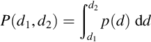
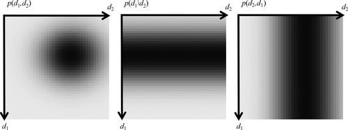
All of the formalism developed in the previous section for discrete probabilities carries over to the case where the observations are continuously changing variables. With just two observations, d₁ and d₂, the probability that the observations are near (d₁, d₂) is described by a two-dimensional probability density function, p(d₁, d₂). Then, the probability, P, that d₁ is between d₁^L and d₁^R, and d₂ is between d₂^L and d₂^R is given as follows:

$P(d_1^L,d_1^R,d_2^L,d_2^R)={\int }_{d_1^L}^{d_1^R}{\int }_{d_2^L}^{d_2^R}p(d_1,d_2)\text{d}{d}_1\text{d}{d}_2$

The probability density function for one datum, irrespective of the value of the other, can be obtained by integration (Figure 3.13):

$p(d_1)={\int }_{d_2^{\text{min}}}^{d_2^{\text{max}}}p(d_1,d_2)\text{d}{d}_2\text{and}p(d_2)={\int }_{d_1^{\text{min}}}^{d_1^{\text{max}}}p(d_1,d_2)\text{d}{d}_1$

Here, d₁^min, d₂^max is the overall range of d₁ and d₂^min, d₂^max is the overall range of d₂. Note that the joint probability density function is normalized so that the total probability is unity:

$P(d_1^{\text{min}},d_1^{\text{max}},d_2^{\text{min}},d_2^{\text{max}})={\int }_{d_1^{\text{min}}}^{d_1^{\text{max}}}{\int }_{d_2^{\text{min}}}^{d_2^{\text{max}}}p(d_1,d_2)\text{d}{d}_1\text{d}{d}_2=1$

The mean and variance are computed in a way exactly analogous to a univariate probability density function:

$\begin{array}{l}{\overline{d}}_1=\int \int d_{1}p(d_1,d_2)\text{d}{d}_1\text{d}{d}_2\text{and}{\overline{d}}_2=\int \int d_{2}p(d_1,d_2)\text{d}{d}_1\text{d}{d}_2\\ {\sigma }_1^2=\int \int {(d_1-{\overline{d}}_1)}^{2}p(d_1,d_2)\text{d}{d}_1\text{d}{d}_2\text{and}{\sigma }_2^2=\int \int {(d_2-{\overline{d}}_2)}^{2}p(d_1,d_2)\text{d}{d}_1\text{d}{d}_2\end{array}$

Note, however, that these formulas can be simplified to just the one-dimensional formulas (Equations 3.3 and 3.4), as the factors multiplying p(d₁, d₂) can be moved outside of one integral. The interior integral then reduces p(d₁, d₂) to p(d₁):

$\begin{array}{ll}{\overline{d}}_1& =\int \int d_{1}p(d_1,d_2)\text{d}{d}_1\text{d}{d}_2=\int d_1\int p(d_1,d_2)\text{d}{d}_2\text{d}{d}_1=\int d_{1}p(d_1)\text{d}{d}_1\\ {\sigma }_1^2& =\int \int {(d_1-{\overline{d}}_1)}^{2}p(d_1,d_2)\text{d}{d}_1\text{d}{d}_2=\int {(d_1-{\overline{d}}_1)}^2\int p(d_1,d_2)\text{d}{d}_2\text{d}{d}_1\\ & =\int {(d_1-{\overline{d}}_1)}^{2}p\left(d_1\right)\text{d}{d}_1\end{array}$

and similarly for ${\overline{d}}_2$ and ${\sigma }_2^2$. In MatLab, we represent the joint probability density function, p(d₁, d₂), as the matrix, P, where d₁ varies along the rows and d₂ along the columns. Normally, we would choose d₁ and d₂ to be evenly sampled with spacing Dd so that they can be represented by column vectors of length, L. A uniform probability density function is then computed as follows:

d1 = Dd*[0:L−1]′;
d2 = Dd*[0:L−1]′;
P = ones(L,L);
norm = (Dd○2)*sum(sum(P));
P = P/norm;

(MatLab eda03_10)

Note that the sum of all the elements of a matrix P is sum(sum(P)). The first sum() returns a row vector of column sums and the second sums up that vector and produces a scalar.

An example of a spatially variable probability density function is

$p(d_1,d_2)=\frac{1}{2\pi {\sigma }_1{\sigma }_2}exp\left\{-\frac{{(d_1-{\overline{d}}_1)}^2}{2{\sigma }_1^2}-\frac{{(d_2-{\overline{d}}_2)}^2}{2{\sigma }_2^2}\right\}$

where ${\overline{d}}_1$, ${\overline{d}}_2$, ${\sigma }_1^2$, and ${\sigma }_2^2$ are constants. This probability density function is a generalization of the Normal probability density functions, and is defined so that the ${\overline{d}}_1$ and ${\overline{d}}_2$ are means and the ${\sigma }_1^2$ and ${\sigma }_2^2$ are variances. We will discuss it in more detail, below. In MatLab, this probability density function is computed:

d1 = Dd*[0:L−1]′;
d2 = Dd*[0:L−1]′;
norm=1/(2*pi*s1*s2);
p1=exp(−((d1−d1bar).○2)/(2*s1*s1));
p2=exp(−((d2−d2bar).○2)/(2*s2*s2));
P=norm*p1*p2′;

(MatLab eda03_11)

Here, d1bar, d2bar, s1, and s2 correspond to ${\overline{d}}_1$, ${\overline{d}}_1$, ${\sigma }_1$, and ${\sigma }_2$, respectively. Note that we have made use here of a vector product of the form, p1*p2′, which creates a matrix, P, whose elements are P_ij = p_ip_j.

In MatLab, the joint probability density function is reduced to a univariate probability density function by using the sum() function to approximate an integral:

% sum along columns, which integrates P along d2 to get p1
p1 = Dd*sum(P,2);
% sum along rows, which integrates P along d1 to get p2
p2 = Dd*sum(P,1)′;

The mean is then calculated as

d1mean = Dd*sum(d1 .* p1 );
d2mean = Dd*sum(d2 .* p2 );

(MatLab eda03_12)

and the variance is computed as

sigma12 = Dd*sum( ((d1-d1mean).○2) .* p1 );
sigma22 = Dd*sum( ((d2-d2mean).○2) .* p2 );

(MatLab eda03_13)

Finally, we define the conditional probability density functions, p(d₁|d₂) and p(d₂|d₁) in a way that is analogous to the discrete case (Figure 3.14). Bayes Theorem then becomes as follows:

$\begin{array}{c}p(d_1|d_2)=\frac{p(d_2|d_1)p(d_1)}{p(d_2)}=\frac{p(d_2|d_1)p(d_1)}{\int p(d_1,d_2)\text{d}{d}_1}=\frac{p(d_2|d_1)p(d_1)}{\int p(d_2|d_1)p(d_1)\text{d}{d}_1}\\ p(d_2|d_1)=\frac{p(d_1|d_2)p(d_2)}{p(d_1)}=\frac{p(d_1|d_2)p(d_2)}{\int p(d_1,d_2)\text{d}{d}_2}=\frac{p(d_1|d_2)p(d_2)}{\int p(d_1|d_2)p(d_2)\text{d}{d}_2}\end{array}$

Here, we have relied on the relations

$\begin{array}{c}p(d_1,d_2)=p(d_1|d_2)p(d_2)\text{and}p(d_1)=\int p(d_1,d_2)\text{d}{d}_2=\int p(d_1|d_2)p(d_2)\text{d}{d}_2\\ p(d_1,d_2)=p(d_2|d_1)p(d_1)\text{and}p(d_2)=\int p(d_1,d_2)\text{d}{d}_1=\int p(d_2|d_1)p(d_1)\text{d}{d}_1\end{array}$

In MatLab, the conditional probability density functions are computed using Equation (3.25):

% sum along columns, which integrates P along d2 to get p1=p(d1)
p1 = Dd*sum(P,2);
% sum along rows, which integrates P along d1 to get p2=p(d2)
p2 = Dd*sum(P,1)′;
% conditional distribution P1g2 = P(d1|d2) = P(d1,d2)/p2
P1g2 = P ./ (ones(L,1)*p2′);
% conditional distribution P2g1 = P(d2|d1) = P(d1,d2)/p1
P2g1 = P ./ (p1*ones(L,1)′);

(MatLab eda03_14)

Note that the MatLab sum() function, when operating on a matrix, returns a column vector of row sums or a row vector of column sums, depending on whether its second argument is 1 or 2, respectively.

3.9 Covariance

In addition to describing the behavior of d₁ and d₂ individually, the joint probability density function p(d₁, d₂) also describes the degree to which they correlate. The sequence of pairs of measurements, (d₁, d₂), might contain a systematic pattern where unusually high values of d₁ occur along with unusually high values of d₂, and unusually low values of d₁ occur along with unusually low values of d₂. In this case, d₁ and d₂ are said to be positively correlated (Figure 3.15). Alternatively, high values of d₁ can occur along with unusually low values of d₂, and unusually low values of d₁ can occur along with unusually high values of d₂. This is a negative correlation. These cases correspond to joint probability density functions, p(d₁, d₂), that have a slanting ridge of high probability. Probability density functions that have neither a positive nor a negative correlation are said to be uncorrelated.

Suppose that we divide the (d₁, d₂) plane into four quadrants of alternating sign, centered on a typical value such as the mean, $({\overline{d}}_1,{\overline{d}}_2)$. A positively correlated probability density function will have most of its probability in the positive quadrants, and a negatively correlated probability density function will have most of its probability in the negative quadrants. This suggests a strategy for quantifying correlation: multiply p(d₁, d₂) by a function, say s(d₁, d₂), that has a four-quadrant alternating sign pattern and integrate (Figure 3.16). The resulting number quantifies the degree of correlation. When $s(d_1,d_2)=(d_1-{\overline{d}}_1)(d_2-{\overline{d}}_2)$, the result is called the covariance, σ_1,2:

${\sigma }_{1,2}=\int \int (d_1-{\overline{d}}_1)(d_2-{\overline{d}}_2)p(d_1,d_2)\text{d}{d}_1\text{d}{d}_2$

In MatLab, the covariance is computed as follows:

% make the alternating sign function
S = (d1−d1bar) * (d2−d2bar)′;
% form the product
SP = S .* P;
% integrate
cov = (Dd○2)*sum(sum(SP));

(MatLab eda03_17)

Here, d1 and d2 are column vectors containing d₁ and d₂ sampled with spacing, Dd.

The variance and covariance can be combined into a single quantity, the covariance matrix, C, by defining

$C_{ij}=\int \int (d_i-{\overline{d}}_i)(d_j-{\overline{d}}_j)p(d_1,d_2)\text{d}{d}_1\text{d}{d}_2$

Its diagonal elements are the variances, σ₁² and σ₂², and its off-diagonal elements are the covariance, σ_1,2. Note that the matrix, C, is symmetric.

3.10 Multivariate distributions

In the previous section, we have examined joint probability density functions of exactly two observations, d₁ and d₂. In practice, the number of observations can be arbitrarily large, (d₁, … d_N). The corresponding multivariate probability density function, p(d₁, … d_N), gives the probability that a set of observations will be in the vicinity of the point (d₁, … d_N). We will write this probability density function as p(d), where d is a column-vector of observations d = [d₁, … d_N]^T. The mean, $\overline{\mathbf{d}}$, is a length-N column-vector whose components are the means of each observation. The covariance matrix, C, is a N × N matrix whose i-th diagonal element is the variance of observation, d_i, and whose (i, j) off-diagonal element is the covariance of observations d_i and d_j.

${\overline{d}}_i=\int d_{i}p(\mathbf{d}){\text{d}}^{\text{N}}d\text{and}{\text{C}}_{ij}=\int (d_i-d_i)(d_j-d_j)p(\mathbf{d}){\text{d}}^{\text{N}}d$

All the integrals are N-dimensional multiple integrals, which we abbreviate here as $\int {\text{d}}^{\text{N}}d$.

3.11 The multivariate Normal distributions

The formula for a N-dimensional Normal probability density function with mean, $\overline{\mathbf{d}}$, and covariance matrix, C, is

$p(\mathbf{d})=\frac{1}{{(2\pi )}^{N/2}|\mathbf{C}{|}^{½}}exp\{-½{(\mathbf{d}-\overline{\mathbf{d}})}^{\text{T}}{\mathbf{C}}^{-1}(\mathbf{d}-\overline{\mathbf{d}})\}$

where |C| is the determinant of the covariance matrix, C, and C⁻¹ is its matrix inverse. This probability density function bears a resemblance to the univariate Normal probability density function (Equation 3.5)—indeed it reduces to it in the N = 1 case. Equation (3.30) can be understood in the following way: The leading factor of (2π)^−N/2|C|^−½ is just a normalization factor, chosen so that $\int p(\mathbf{d}){\text{d}}^{\text{N}}d=1$. The rest of the equation is the key part of the Normal curve, and contains, as expected, an exponential whose argument is quadratic in d. The most general quadratic that can be formed from d is $(\mathbf{d}-\mathbf{d}\mathbf{\prime })\mathbf{M}{(\mathbf{d}-\mathbf{d}\mathbf{\prime })}^{\text{T}}$, where d’ is an arbitrary vector and M is an arbitrary matrix. The specific choices $\mathbf{d}\mathbf{\prime }=\overline{\mathbf{d}}$ and M = C⁻¹ are controlled by the desire to have the mean and covariance of the probability density function be exactly $\overline{\mathbf{d}}$ and C, respectively. Therefore, we need only to convince ourselves that Equation (3.30) has the requisite total probability, mean, and covariance.

Surprisingly, given the complexity of Equation (3.30), these requirements can be easily checked by direct calculation. All that is necessary is to transform the probability density function to the new variable $\mathbf{y}={\mathbf{C}}^{-½}(\mathbf{d}-\overline{\mathbf{d}})$ and perform the requisite integrations. However, in order to proceed, we need to recall that the rule for transforming a multidimensional integral (the analog to Equation 3.7) is

$\int p(\mathbf{d}){\text{d}}^{\text{N}}d=\int p(\mathbf{d}(\mathbf{y}))|\frac{\partial \mathbf{d}}{\partial \mathbf{y}}|{\text{d}}^{\text{N}}y=\int p(\mathbf{d}(\mathbf{y}))J(\mathbf{y}){\text{d}}^{\text{N}}y$

where $J(\mathbf{y})=|\partial \mathbf{d}/\partial \mathbf{y}|$ is the Jacobian determinant; that is, the determinant of the matrix whose elements are $\partial d_{\text{i}}/\partial y_{\text{j}}$. (The rule, ${\text{d}}^{\text{N}}d=|\partial \mathbf{d}/\partial \mathbf{y}|{\text{d}}^{\text{N}}y$ is a multidimensional generalization of the ordinary chain rule, dd = |dd/dy|dy). In our case, $\mathbf{y}={\mathbf{C}}^{-½}(\mathbf{d}-\overline{\mathbf{d}})$ and $|\partial \mathbf{d}/\partial \mathbf{y}|=|\mathbf{C}{|}^{½}$. Then, the area under p(d) is

$\begin{array}{ll}\int p(\mathbf{d}){\text{d}}^{\text{N}}d& =\frac{1}{{(2\pi )}^{N/2}|\mathbf{C}{|}^{½}}\int exp\{-½{\mathbf{y}}^T\mathbf{y}\}{|\mathbf{C}|}^{½}{\text{d}}^{\text{N}}y\\ & =\frac{1}{{(2\pi )}^{N/2}}\int exp\{-½{\mathbf{y}}^T\mathbf{y}{\}\text{d}}^{\text{N}}y\\ & ={\prod }_{i=1}^N\int \frac{1}{{(2\pi )}^{½}}exp\{-½y_i^2\}\text{d}{y}_i={\prod }_{i=1}^{N}1=1\end{array}$

Note that the factor of |C|^½ arising from the Jacobian determinant cancels the |C|^−½ in the normalization factor. As the final integral is just a univariate Normal probability density function with zero mean and unit variance, its integral (total area) is unity. We omit here the integrals for the mean and covariance. They are algebraically more complex but are performed in an analogous fashion.

We run into a notational difficulty when computing a multivariate Normal probability density function in MatLab, of the sort that is frequently encountered when coding numerical algorithms. Heretofore, we have been using column vectors starting with lower-case “d” names, such as d1 and d2, to represent quantities sampled at L evenly spaced increments (d₁ and d₂ in this case). Now, however, the equation for the Normal probability density function (Equation 3.30) requires us to group corresponding ds into an N-vector, d = [d₁, d₂, … d_N]^T, which appears in the matrix multiplication, ${(\mathbf{d}-\overline{\mathbf{d}})}^T{\mathbf{C}}^{-1}(\mathbf{d}-\overline{\mathbf{d}})$. Thus, we are tempted to define quantities that will also have lower-case “d” names, but will be N-vectors, which violates the naming convention. Furthermore, the MatLab syntax becomes more inscrutable, for the N × N matrix multiplication needs to be performed at each of L² combinations of (d₁, d₂) in order to evaluate p(d₁, d₂) on a L × L grid. There is no really good way around these problems, but we put forward two different strategies for dealing with them.

The first is to use only L-vectors, and explicitly code the N × N matrix multiplication, instead of having MatLab perform it. The N = 2 case needed for the two-dimensional probability density function p(d₁, d₂) is

${(\mathbf{d}-\overline{\mathbf{d}})}^T{\mathbf{C}}^{-1}(\mathbf{d}-\overline{\mathbf{d}})={[{\mathbf{C}}^{-1}]}_{11}{({\text{d}}_1-{\overline{\mathbf{d}}}_1)}^2+{[{\mathbf{C}}^{-1}]}_{22}{({\text{d}}_2-{\overline{\mathbf{d}}}_2)}^2+2{[{\mathbf{C}}^{-1}]}_{12}({\text{d}}_1-{\overline{\mathbf{d}}}_1)({\text{d}}_2-{\overline{\mathbf{d}}}_2)$

Note that we have made use of the fact that the covariance matrix, C, is symmetric. The MatLab code for the Normal probability density function is then

CI=inv(C);
norm=1/(2*pi*sqrt(det(C)));
dd1=d1−d1bar;
dd2=d2−d2bar;
P=norm*exp(−0.5*CI(1,1)*(dd1.○2)*ones(N,1)′ …
 −0.5*CI(2,2)*ones(N,1)*(dd2.○2)′ …
 −CI(1,2)*dd1*dd2′);

(MatLab eda03_15)

Here, C is the covariance matrix, and d1 and d2 are d₁ and d₂ sampled at L evenly spaced increments.

The second strategy is to define both L-vectors and N-vectors and to use the N-vectors to compute ${(\mathbf{d}-\overline{\mathbf{d}})}^T{\mathbf{C}}^{-1}(\mathbf{d}-\overline{\mathbf{d}})$ using the normal MatLab syntax for matrix multiplication. In the N = 2 case, the 2-vectors must be formed explicitly for each of the L × L pairs of (d₁, d₂), which is best done inside a pair of for loops:

CI=inv(C);
norm=1/(2*pi*sqrt(det(C)));
P=zeros(L,L);
for i = [1:L]
for j = [1:L]
dd = [d1(i)−d1bar, d2(j)−d2bar]′;
P(i,j)=norm*exp(−0.5 * dd′ * CI * dd );
end
end

(MatLab eda03_16)

The outer for loop corresponds to the L elements of d1 and the inner to the L elements of d2. The code for the second method is arguably a little more transparent than the code for the first, and is probably the better choice, especially for beginners.

3.12 Linear functions of multivariate data

Suppose that a column-vector of model parameters, m, is derived from a column-vector of observations, d, using the linear formula, m = Md, where M is some matrix. Suppose that the observations are random variables with a probability density function, p(d), with mean, $\overline{\mathbf{d}}$, and covariance, C_d. The model parameters are random variables too, with probability density function, p(m). We would like to derive the functional form of the probability density function, p(m), as well as calculate its mean, $\overline{\mathbf{m}}$, and covariance, C_m.

If p(d) is a Normal probability density function, then p(m) is also a Normal probability density function, as can be seen by transforming p(d) to p(m) using the rule (see Equation 3.31):

$p(\mathbf{d})=p(\mathbf{d}(\mathbf{m}))\left|\frac{\partial \mathbf{d}}{\partial \mathbf{m}}\right|=p(\mathbf{d}(\mathbf{m}))J(\mathbf{m})$

As m = Md, the Jacobian determinant is $J(\mathbf{m})=|\partial \mathbf{d}/\partial \mathbf{m}|=|{\mathbf{M}}^{-1}|={|\mathbf{M}|}^{-1}$. Then:

$\begin{array}{ll}\hfill p(\mathbf{m})& =p\left(\mathbf{d}\left(\mathbf{m}\right)\right)J\left(\mathbf{m}\right)\hfill \\ \hfill & =\frac{1}{{(2\pi )}^{N/2}{|{\mathbf{C}}_d|}^{½}|\mathbf{M}|}exp\{-½{({\mathbf{M}}^{-1}\mathbf{m}-{\mathbf{M}}^{-1}\mathbf{M}\overline{\mathbf{d}})}^{\text{T}}{\mathbf{C}}_d^{-1}({\mathbf{M}}^{-1}\mathbf{m}-{\mathbf{M}}^{-1}\mathbf{M}\overline{\mathbf{d}})\}\hfill \\ \hfill & =\frac{1}{{(2\pi )}^{N/2}{|\mathbf{M}{\mathbf{C}}_d{\mathbf{M}}^{\text{T}}|}^{½}}exp\{-½{(\mathbf{m}-\mathbf{M}\overline{\mathbf{d}})}^{\text{T}}[{\mathbf{M}}^{-1\text{T}}{\mathbf{C}}_d^{-1}{\mathbf{M}}^{-1}](\mathbf{m}-\mathbf{M}\overline{\mathbf{d}})\}\hfill \\ \hfill & =\frac{1}{{(2\pi )}^{N/2}|{\mathbf{C}}_m|½}exp\{-½{(\mathbf{m}-\overline{\mathbf{m}})}^{\text{T}}{\mathbf{C}}_m^{-1}(\mathbf{m}-\overline{\mathbf{m}})\}\hfill \\ \text{where}\overline{\mathbf{m}}\hfill & =\mathbf{M}\overline{\mathbf{d}}\text{and}{\mathbf{C}}_m^{-1}={\mathbf{M}}^{-1\text{T}}{\mathbf{C}}_d^{-1}{\mathbf{M}}^{-1}& \hfill \end{array}$

Note that we have used the identities (AB)^T = B^TA^T, (AB)⁻¹ = B⁻¹A⁻¹, |AB| = |A| |B|, |C^T| = |C|, and |C⁻¹| = |C|⁻¹. Thus, the transformed mean and covariance matrix are given by the simple rule

$\overline{\mathbf{m}}=\mathbf{M}\overline{\mathbf{d}}\text{and}{\mathbf{C}}_{\mathbf{m}}=\mathbf{M}{\mathbf{C}}_d{\mathbf{M}}^{\text{T}}$

Equation (3.36) is very important, for it shows how to calculate the mean and covariance matrix of the model parameters, given the mean and variance of the data. The covariance formula,${\mathbf{C}}_m=\mathbf{M}{\mathbf{C}}_d{\mathbf{M}}^{\text{T}}$, can be thought of as a rule for error propagation. It links error in the data to error in the model parameters. The rule is shown to be true even when M is not square and when M⁻¹ does not exist (see Note 3.1).

As an example, consider the case where we measure the masses of two objects A and B, by first putting A on a scale and then adding B, without first removing A. The observation, d₁, is the mass of object A and the observation d₂ is the combined mass of objects A and B. We assume that the measurements are a random process with probability density function p(d₁, d₂), with means ${\overline{d}}_1$ and ${\overline{d}}_2$, variance, σ_d², and covariance, σ_1,2 = 0. Note that both variances are the same, indicating that both measurements have the same amount of error, and that the covariance is zero, indicating that the two measurements are uncorrelated. Suppose that we want to compute the mass of object B and the difference in masses of objects B and A. Then, B = (B + A) − A → m₁ = d₂ − d₁, and B − A = (B + A) − 2A → m₂ = d₂ − 2d₁. The matrix, M, is given by

$\mathbf{M}=\left[\begin{array}{cc}-1& 1\\ -2& 1\end{array}\right]$

The mean is

$\overline{\mathbf{m}}=\mathbf{M}\overline{\mathbf{d}}=\left[\begin{array}{cc}-1& 1\\ -2& 1\end{array}\right]\left[\begin{array}{c}{\overline{d}}_1\\ {\overline{d}}_2\end{array}\right]\text{or}{\overline{m}}_1={\overline{d}}_2-{\overline{d}}_1\text{and}{\overline{m}}_2={\overline{d}}_2-2{\overline{d}}_1$

The covariance matrix is

$\begin{array}{c}{\mathbf{C}}_m=\mathbf{M}{\mathbf{C}}_d{\mathbf{M}}^{\text{T}}=\left[\begin{array}{cc}-1& 1\\ -2& 1\end{array}\right]\left[\begin{array}{cc}{\sigma }_d^2& 0\\ 0& {\sigma }_d^2\end{array}\right]\left[\begin{array}{cc}-1& -2\\ 1& 1\end{array}\right]={\sigma }_d^2\left[\begin{array}{cc}2& 3\\ 3& 5\end{array}\right]\\ \text{or}\\ {\sigma }_{m_1}^2=2{\sigma }_d^2\text{and}{\sigma }_{m_2}^2=5{\sigma }_d^2\text{and}{\sigma }_{m1,2}=3{\sigma }_d^2\end{array}$

Note that the ms have unequal variance even though the variances of the ds are equal, and that the ms have a non-zero covariance even though the covariance of the ds is zero (Figure 3.17). This process of forming model parameters from data often results in variances and degrees of correlation that are different from the underlying data. Depending on the situation, variance can be either reduced (good) or amplified (bad). While data are often observed through a measurement process that has uncorrelated errors (good), the model parameters formed from them usually exhibit strong correlations (not so good).

The rule for the mean and variance (Equation 3.36) is true even when the underlying probability density function, p(m), is not Normal, as can be verified by a calculation analogous to that of Equations (3.9) and (3.10):

$\begin{array}{ll}{\overline{m}}_i& =\int m_{i}p(\mathbf{m}){\text{d}}^{N}m\\ & =\int \sum _j{M}_{ij}{d}_{j}p(\mathbf{d}){\text{d}}^{N}d\\ & =\sum _j{M}_{ij}\int d_{j}p(\mathbf{d})d^{N}d=\sum _j{M}_{ij}{\overline{d}}_j\text{or}\overline{\mathbf{m}}=\mathbf{M}\overline{\mathbf{d}}\end{array}$

$\begin{array}{ll}{[{\mathbf{C}}_{\mathbf{m}}]}_{ij}& =\int (m_i-{\overline{m}}_i)(m_j-{\overline{m}}_j)p(\mathbf{m})d^{N}m\\ & =\int \sum _p{M}_{ip}(d_p-{\overline{d}}_p)\sum _q{M}_{jq}(d_q-{\overline{d}}_q)p(\mathbf{d}){\text{d}}^{N}d\\ & =\sum _p{M}_{ip}{\sum }_q{M}_{jq}\int (d_p-{\overline{d}}_p)(d_q-{\overline{d}}_q)p(\mathbf{d}){\text{d}}^{N}d\\ & =\sum _p{M}_{ip}{\sum }_q{M}_{jq}{[{\mathbf{C}}_m]}_{pq}\text{or}{\mathbf{C}}_m=\mathbf{M}{\mathbf{C}}_d{\mathbf{M}}^{\text{T}}\end{array}$

Here, we have used the fact that

$p(\mathbf{m})d^{N}m=p(\mathbf{m}(\mathbf{d}))|\partial \mathbf{m}/\partial \mathbf{d}||\partial \mathbf{d}/\partial \mathbf{m}|{\text{d}}^{\text{N}}d=p(\mathbf{d}){\text{d}}^{\text{N}}d.$

In the case of non-Normal probability density functions, these results need to be used cautiously. The relationship between variance and confidence intervals (e.g., the amount of probability falling between m₁ − σ_m1 and m₁ + σ_m1) varies from one probability density function to another.

Even in the case of Normal probability density functions, statements about confidence levels need to be made carefully, as is illustrated by the following scenario. Suppose that p(d₁, d₂) represents the joint probability density function of two measurements, say the height and length of an organism, and suppose that these measurements are uncorrelated with equal variance, σ_d². As we might expect, the univariate probability density function $p(d_1)=\int p(d_1,d_2)\text{d}{d}_2$, has variance, σ_d², and so the probability, P₁, that d₁ falls between d₁ − σ_d and d₁ + σ_d is 0.6827 or 68.27%. Likewise, the probability, P₂, that d₂ falls between d₂ − σ_d and d₂ + σ_d is also 0.6827 or 68.27%. But P₁ represents the probability of d₁ irrespective of the value of d₂ and P₂ represents the probability of d₂ irrespective of the value of d₁. The probability, P, that both d₁ and d₂ simultaneously fall within their respective one-sigma confidence intervals is P = P₁P₂ = (0.6827)² = 0.4660 or 46.60%, which is significantly smaller than 68.27%.

Problems

3.1 The univariate probability density function p(d) = c(1 − d) is defined on the interval 0 ≤ d ≤ 1. (A) What must the constant, c, be for the probability density function to be properly normalized? (B) Calculate the mode, median, and mean of this probability density function analytically.

3.2 The univariate exponential probability density function is p(d) = λexp(−λd) where d is defined on the interval 0 ≤ d < ∞. The parameter, λ, is called the rate parameter. (A) Use MatLab to plot shaded column-vectors of this probability density function and to compute its mode, median, mean, and variance, for the cases λ = 5 and λ = 10. (B) Is it possible to control the mean and variance of this probability density function separately?

3.3 Suppose that p(d) is a Normal probability density function with zero mean and unit variance. (A) Derive the probability density function of m = |d|^½, analytically. (B) Use MatLab to plot shaded column-vectors of this probability density function and to compute its mode, median, mean, and variance.

3.4 Suppose that a corpse is brought to a morgue and the coroner is asked to assess the probability that the cause of death was pancreatic cancer (as contrasted to some other cause of death). Before examining the corpse, the best estimate that the coroner can make is 1.4%, the death rate from pancreatic cancer in the general population. Now suppose the coroner performs a test for pancreatic cancer that is 99% accurate, both in the sense that if the cause of death was pancreatic cancer, the probability is 99% that the test results are positive, and if the cause of death was something else, the probability is 99% that the test results are negative. Let the cause of death be represented by the variable, D, which can take two discrete values, C, for pancreatic cancer and E, for something else. The test is represented by the variable, T, which can take two values, Y for positive and N for negative. (A) Write down the 2 × 2 table of the conditional probabilities P(D|T). (B) Suppose the test results are negative. Use Bayesian Inference to assess the probability that the cause of death was pancreatic cancer. (C) How can the statement that the test is 99% accurate be used in a misleading way?

3.5 Suppose that two measurements, d₁ and d₂, are uncorrelated and with equal variance, σ_d². What is the variance and covariance of two model parameters, m₁ and m₂, that are the sum and difference of the ds?

3.6 Suppose that the vectors, d, of N measurements are uncorrelated and with equal variance, σ_d². (A) What is the form of the covariance matrix, C_d? (B) Suppose that m = Md. What property must M have to make the m's, as well as the d's, uncorrelated? (C) Does the matrix from Problem 3.5 have this property?