10.1 Interpolation requires prior information

Two situations in which data points need to be filled in are common:

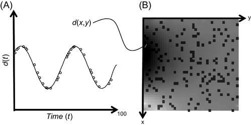
In both cases, the times or positions at which the data have been observed are inconvenient. A solution to this dilemma is to interpolate the data; that is, to use the available data to estimate the data values at a more useful set of times or positions. We encountered the interpolation problem previously, in Chapter 5 (see Figure 10.1). Prior information about how the data behaved between the data points was a key factor in achieving the result.

The generalized least-squares methodology that we developed in Chapter 5 utilized both observations and the prior information to create an estimate of the data at all times or positions. Observations and prior information are both treated probabilistically. The solution is dependent on the observations and prior information, but does not satisfy either, anywhere. This is not seen as a problem, because both observations and prior information are viewed as subject to uncertainty. There is really no need to satisfy either of them exactly; we only need to find a solution for which the level of error is acceptable.

An alternative, deterministic approach is to find a solution that passes exactly through the observations and that exactly satisfies the prior information between them. Superficially, this approach seems superior—both observations and prior information are being satisfied exactly. However, this approach singles out the observation points as special. The solution will inevitably behave somewhat differently at the observation points than between them, which is not a desirable property.

Whether or not this approach is tractable—or even possible—depends on the type of prior information involved. Information about smoothness turns out to be especially easy to implement and leads to a set of techniques that might be called the traditional approach to interpolation. As we will see, these techniques are a straightforward extension of the linear model techniques that we have been developing in this book.

A purist might argue that interpolation of any kind is never the best approach to data analysis, because it will invariably introduce features not present in the original data, leading to wrong conclusions. A better approach is to generalize the analysis technique so that it can handle irregularly spaced data. This argument has merit, because interpolation adds additional—and often unquantifiable—error to the data. Nevertheless, if used sensibly, it is a valid data analysis tool that can simplify many data processing projects.

The basic idea behind interpolation is to construct an interpolant, a function, d(t), that goes through all the data points, d_i, and does something sensible in between them. We can then evaluate the interpolant, d(t), at whatever values of time, t, that we want—evenly spaced times, or times that match those of another dataset, to name two examples. Finding functions that go through a set of data points is easy. Finding functions that do something sensible in between the data points is more difficult as well as more problematical, because our notion of what is sensible will depend on prior knowledge, which varies from dataset to dataset.

Some obvious ideas do not work at all. A polynomial of degree N − 1, for instance, can easily be constructed to go through N data points (Figure 10.2). Unfortunately, the polynomial often takes wilds swings between the points. A high-degree polynomial does not embody the prior information that the function, d(t), does not stray too far above or below the values of nearby data points.

10.2 Linear interpolation

A low-order polynomial is less wiggly than a high-order one and is better able to capture the prior information of smoothness. Unfortunately, a low-order polynomial can pass exactly through only a few data. The solution is to construct the function, d(t), out of a sequence of polynomials, each valid for a short time interval. Such functions are called splines.

The simplest splines are line segments connecting the data points. The second derivative of a line is zero, so it embodies the prior information that the function is very smooth between the data points. The estimated datum at time, t, depends only on the values of the two bracketing observations, the one made immediately before time, t, and the one immediately after time, t. The interpolation formula is as follows:

$\begin{array}{c}\text{estimated datum}=\text{weighted average of bracketing observations}\\ \text{or}\\ d(t)=\frac{(t_{i+1}-t)d_i}{h_i}+\frac{(t-t_i)d_{i+1}}{h_i}\text{with}{h}_i=t_{i+1}-t_i\end{array}$

Here, the time, t, is bracketed by the two observation times, t_i and t_i+1. Note the use of the local quantities, t_i+1 − t and t − t_i; that is, time measured with respect to a nearby sample. In MatLab, linear interpolation is performed as follows:

dp=interp1(t,d,tp);

(MatLab eda10_02)

Here, d is a column vector of the original data, measured at time, t, and dp is the interpolated data at time, tp.

Linear interpolation has the virtue of being simple. The interpolated data always lie between the observed data; they never deviate above or below them (Figure 10.3). Its major defect is that the function, d(t), has kinks (discontinuities in slope) at the data points. The kinks are undesirable because they are an artifact not present in the original data; they arise from the prior information. Kinks will, for instance, add high frequencies to the power spectral density of the time series.

10.3 Cubic interpolation

A relatively simple modification is to use cubic polynomials in each of the intervals between the data points, instead of linear ones. A cubic polynomial has four coefficients and can satisfy four constraints. The requirement that the function must pass through the observed data at the ends of the interval places two constraints on these coefficients, leaving two constraints that can represent prior information. We can require that the first and second derivatives are continuous across intervals, creating a smooth function, d(t), that has no kinks across intervals. (Its first derivative has no kinks either, but its second derivative does).

The trick behind working out simple formula for cubic splines is properly organizing the knowns and the unknowns. We start by defining the i-th interval as the one between time, t_i, and time, t_i+1. Within this interval, the spline function is a cubic polynomial, S_i(t). As the second derivative of a cubic is linear, it can be specified by its values, y_i and y_i+1, at the ends of the interval:

$\begin{array}{c}\text{second derivative}=\text{weighted average of bracketing values}\\ \text{or}\\ \frac{d^2}{d{t}^2}{S}_i(t)=\frac{y_i(t_{i+1}-t)}{h_i}+\frac{y_{i+1}(t-t_i)}{h_i}\text{with}{h}_i=t_{i+1}-t_i\end{array}$

(Compare with Equation 10.1). We can make the second derivative continuous across adjacent intervals if we equate y_i of interval i + 1 with y_i+1 of interval i. Thus, only one second derivative, y_i, is defined for each time, t_i, even though two cubic polynomials touch this point. These ys are the primary unknowns in this problem. The formula for S_i(t) can now be found by integrating Equation 10.2 twice:

$S_i(t)=\frac{y_i{(t_{i+1}-t)}^3}{6h_i}+\frac{y_{i+1}{(t-t_i)}^3}{6h_i}+a_i(t_{i+1}-t)+b_i(t-t_i)$

Here a_i and b_i are integration constants. We now choose these constants so that the cubic goes through the data points, that is S_i(t_i) = d_i and S_i(t_i+1) = d_i+1. This requirement leads to

$\begin{array}{l}{S}_i(t_i)=d_i=\frac{y_i{h_i}^2}{6}+a_i{h}_i\text{or}{a}_i=\frac{d_i}{h_i}-\frac{y_i{h}_i}{6}\hfill \\ S_i(t_{i+1})=d_{i+1}=\frac{y_{i+1}{h_i}^2}{6}+b_i{h}_i\text{or}{b}_i=\frac{d_{i+1}}{h_i}-\frac{y_{i+1}{h}_i}{6}\hfill \end{array}$

The cubic spline is then

$S_i(t)=\frac{y_i{(t_{i+1}-t)}^3}{6h_i}+\frac{y_{i+1}{(t-t_i)}^3}{6h_i}+\left(\frac{d_i}{h_i}-\frac{y_i{h}_i}{6}\right)(t_{i+1}-t)+\left(\frac{d_{i+1}}{h_i}-\frac{y_{i+1}{h}_i}{6}\right)(t-t_i)$

and its first derivative is

$\begin{array}{ll}\frac{d}{dt}{S}_i(t)\hfill & =-\frac{y_i{(t_{i+1}-t)}^2}{2h_i}+\frac{y_{i+1}{(t-t_i)}^2}{2h_i}-\left(\frac{d_i}{h_i}-\frac{y_i{h}_i}{6}\right)+\left(\frac{d_{i+1}}{h_i}-\frac{y_{i+1}{h}_i}{6}\right)\hfill \\ \hfill & =-\frac{y_i{(t_{i+1}-t)}^2}{2h_i}+\frac{y_{i+1}{(t-t_i)}^2}{2h_i}+\frac{(d_{i+1}-d_i)}{h_i}-\frac{(y_{i+1}-y_i)h_i}{6}\hfill \end{array}$

Finally, we determine the ys by requiring that two neighboring splines have first derivatives that are continuous across the interval:

$\begin{array}{c}\frac{d}{dt}{S}_{i-1}(t_i)=\frac{d}{dt}{S}_i(t_i)\\ \text{or}\\ \frac{y_i{h}_{i-1}}{2}+\frac{(d_i-d_{i-1})}{h_{i-1}}-\frac{(y_i-y_{i-1})h_{i-1}}{6}=-\frac{y_i{h}_i}{2}+\frac{(d_{i+1}-d_i)}{h_i}-\frac{(y_{i+1}-y_i)h_i}{6}\\ \text{or}\\ h_{i-1}{y}_{i-1}+2(h_{i-1}+h_i)y_i+h_i{y}_{i+1}=\frac{6(d_{i+1}-d_i)}{h_i}-\frac{6(d_i-d_{i-1})}{h_{i-1}}\end{array}$

The y's satisfy a linear equation that can be solved by standard matrix methods, which we have discussed in Chapter 1. Note that the i = 1 and i = N equations involve the quantities, y₀ and y_N+1, which represent the second derivatives at two undefined points, one to the left of the first data point and the other to the right of the last data point. They can be set to any value and moved to the right hand side of the equation. The choice y₀ = y_N+1 = 0 leads to a solution called natural cubic splines.

Because of its smoothness (Figure 10.4), cubic spline interpolation is usually preferable to linear interpolation.

In MatLab, cubic spline interpolation is performed as follows:

dp=spline(t,d,tp);

(MatLab eda10_03)

Here, d is a column vector of the original data, measured at time, t, and dp is the interpolated data at time, tp.

10.4 Kriging

The generalized least-squared methodology that we developed in Chapter 5 to fill in data gaps was based on prior information, represented by the linear equation, $\mathbf{Hm}=\overline{\mathbf{h}}$. We quantified roughness, say R, of a vector, m, by choosing H to be a matrix of second derivatives and by setting $\overline{\mathbf{h}}$ to zero. The minimization of the total roughness,

$R={(\mathbf{Hm})}^{\text{T}}(\mathbf{Hm})$

in Equation (5.8) leads to a solution that is smooth. Note that we can rewrite Equation (10.8) as

$R={(\mathbf{Hm})}^{\text{T}}(\mathbf{Hm})={\mathbf{m}}^{\text{T}}{\mathbf{H}}^{\text{T}}\mathbf{H}\mathbf{m}={\mathbf{m}}^{\text{T}}{[{\mathbf{C}}_m]}^{-1}\mathbf{m}\text{with}{\mathbf{C}}_m={[{\mathbf{H}}^{\mathbf{T}}\mathbf{H}]}^{-1}$

We have encountered the quantity, ${\mathbf{m}}^{\text{T}}{[{\mathbf{C}}_m]}^{-1}\mathbf{m}$, before in Equation (5.1), where we interpreted it as the error, E_p(m), in the prior information. The quantity, ${\mathbf{C}}_{\mathbf{m}}={[{\mathbf{H}}^{\text{T}}\mathbf{H}]}^{-1}$, can be interpreted as the covariance, C_m, of the prior information. In the case of smoothness, the prior covariance matrix, C_m, has nonzero off-diagonal elements. Neighboring model parameters are highly correlated, as a smooth curve is one for which neighboring points have similar values. Thus, the prior covariance, C_m, of the model is intrinsically linked to the measure of smoothness. Actually we have already encountered this link in the context of time series. The autocorrelation function of a time series is closely related to both its covariance and its smoothness (see Section 9.1). This analysis suggests that prior information about a function's autocorrelation function can be usefully applied to the interpolation problem.

Kriging (named after its inventor, Danie G. Krige) is an interpolation method based on this idea. It provides an estimate of a datum, $d_0^{\text{est}}$, at an arbitrary time, $t_0^{\text{est}}$, based on a set of N observations, say $(t_i^{\text{obs}},d_i^{\text{obs}})$, when prior information about its autocorrelation function, a(t), is available. The method assumes a linear model in which $d_0^{\text{est}}$ is a weighted average of all the observed data (as contrasted to just the two bracketing data) (Krige, 1951):

$\begin{array}{ll}\text{estimated datum}\hfill & =\text{weighted average of all observations}\hfill \\ d_0^{\text{est}}={\sum }_{i=1}^N{w}_i{d}_i^{\text{obs}}\hfill & ={({\mathbf{d}}^{\text{obs}})}^{\text{T}}\mathbf{w}\hfill \end{array}$

Here, d^obs is a column vector of the observed data and w is an unknown column-vector of weights. As we shall see, the weights can be determined using prior knowledge of the autocorrelation function. The approach is to minimize the variance of $d_0^{\text{est}}-d_0^{\text{true}}$, the difference between the estimated and true value of the time series. As we will see, we will not actually need to know the true value of the time series, but only its true autocorrelation function. The formula for variance is

$\begin{array}{ll}{\sigma }_{\mathrm{\Delta }d}^2\hfill & =\int {[(d_0^{\text{est}}-d_0^{\text{true}})-({\overline{d}}_0^{\text{est}}-{\overline{d}}_0^{\text{true}})]}^{2}p(\mathbf{d}){\text{d}}^{N}d=\int {(d_0^{\text{est}}-d_0^{\text{true}})}^{2}p(\mathbf{d}){\text{d}}^{N}d\hfill \\ \hfill & =\int {(d_0^{\text{est}})}^{2}p(\mathbf{d}){\text{d}}^{N}d+\int {(d_0^{\text{true}})}^{2}p(\mathbf{d}){\text{d}}^{N}d-2\int d_0^{\text{est}}{d}_0^{\text{true}}p(\mathbf{d}){\text{d}}^{N}d\hfill \\ \hfill & =\sum _{i=1}^N\sum _{j=1}^N{w}_i{w}_j\int d_i^{\text{obs}}{d}_i^{\text{obs}}p(\mathbf{d}){\text{d}}^{N}d+\int {(d_0^{\text{true}})}^{2}p(\mathbf{d}){\text{d}}^{N}d-2\sum _{i=1}^N{w}_i\int d_0^{\text{est}}{d}_j^{\text{true}}p(\mathbf{d}){\text{d}}^{N}d\hfill \end{array}$

Here, p(d) is the probability density function of the data. We have assumed that the estimated and true data have the same mean, that is, ${\overline{d}}_0^{\text{est}}={\overline{d}}_0^{\text{true}}$. We now set $d_i^{\text{obs}}\approx d_i^{\text{true}}$ so that

${\sigma }_{\mathrm{\Delta }d}^2\propto \sum _{i=1}^N\sum _{j=1}^N{w}_i{w}_{j}a(|t_j^{\text{obs}}-t_i^{\text{obs}}|)+a(0)-2\sum _{i=1}^N{w}_{i}a(|t_i^{\text{obs}}-t_0|)$

Note that we have used the definition of the autocorrelation function, a(t) (see Equation 9.6) and that we have ignored a normalization factor (hence the ∝ sign), which appears in all three terms of the equation. Finally, we differentiate the variance with respect to w_k and set the result to zero:

$\frac{d{\sigma }_{\mathrm{\Delta }d}^2}{d{w}_k}=0\propto 2\sum _{j=1}^N{w}_{i}a(|t_k^{\text{obs}}-t_i^{\text{obs}}|)-2a(|t_k^{\text{obs}}-t_0|)$

which yields the matrix equation

$\mathbf{Mw}=\mathbf{v}\text{where}{M}_{\mathit{ij}}=a(|t_i^{\text{obs}}-t_j^{\text{obs}}|)\text{and}{v}_i=a(|t_i^{\text{obs}}-t_0^{\text{est}}|)$

Thus,

$\mathbf{w}={\mathbf{M}}^{-1}\mathbf{v}\text{and}{d}_0^{\text{est}}={({\mathbf{d}}^{\text{obs}})}^{\text{T}}\mathbf{w}={({\mathbf{d}}^{\text{obs}})}^{\text{T}}{\mathbf{M}}^{-1}\mathbf{v}$

Note that the matrix, M, and the column-vector, v, depend only on the autocorrelation of the data. Normally, data needs to be interpolated at many different times, not just one as in the equation above. In such case, we define a column vector, t₀^est, of all the times at which it needs to be evaluated, along with a corresponding vector of interpolated data, d₀^est. The solution becomes

${\mathbf{d}}_0^{\text{est}}={({\mathbf{d}}^{\text{obs}})}^{\text{T}}{\mathbf{M}}^{-1}\mathbf{V}\text{with}{[\mathbf{V}]}_{\mathit{ij}}=a(|t_i^{\text{obs}}-{[{\mathbf{t}}_0^{\text{est}}]}_j|)$

Note that the results are insensitive to the overall amplitude of the autocorrelation function, which cancels from the equation; only its shape matters. Prior notions of smoothness are implemented by specifying a particular autocorrelation function. A wide autocorrelation function will lead to a smooth estimate of d(t) and a narrow function to a rough one. For instance, if we use a Normal function,

$a\left(|t_i-t_j|\right)=\text{exp}\left\{-\frac{{(t_i-t_j)}^2}{2L^2}\right\}$

then its variance, L, will control the degree of smoothness of the estimate.

In MatLab, this approach is very simply implemented:

A = exp(−abs(tobs*ones(N,1)’−ones(N,1)*tobs’).^2/(2*L2));
V = exp(−abs(tobs*ones(M,1)’−ones(N,1)*test’).^2/(2*L2));
dest=dobs′*((A+1e−6*eye(N))V);

(MatLab eda10_04)

Note that we have damped the matrix, A, by addition of a small amount of the identity matrix. This modification guards against the possibility that the matrix, A, is near-singular. It has little effect on the solution when it is not near-singular, but drives the solution towards zero when it is. An example is shown in Figure 10.5.

Finally, we note that the power spectral density of a time series is uniquely determined by its autocorrelation function, as the former is the Fourier transform of the latter (see Section 9.3). Thus, while we have focused here on prior information in the form of the autocorrelation function of the time series, we could alternatively have used prior information about its power spectral density.

10.5 Interpolation in two-dimensions

Interpolation is not limited to one dimension. Equally common is the case where data are collected on an irregular two-dimensional grid but need to be interpolated onto a regular, two-dimensional grid. The basic idea behind two-dimensional interpolation is the same as in one dimension: construct a function, d(x₁, x₂), that goes through all the data points and does something sensible in between them, and use it to estimate the data at whatever points, (x₁, x₂), are of interest.

A key part of spline interpolation is defining intervals over which the spline functions are valid. In one-dimensional interpolation, the intervals are both conceptually and computationally simple. They are just the segments of the time axis bracketed by neighboring observations. As long as the data are in the order of increasing time, each interval is between a data point and its successor. In two dimensions, intervals become two-dimensional patches (or tiles) in (x₁, x₂). Creating and manipulating these tiles is complicated.

One commonly used tiling is based on connecting the observation points together with straight lines, to form a mesh of triangles. The idea is to ensure that the vertices of every triangle coincide with the data points and that the (x₁, x₂) plane is completely covered by triangles with no holes or overlap. A spline function is then defined within each triangle. Such triangular meshes are nonunique as the data points can be connected in many alternative ways. Delaunay triangulation is a method for constructing a mesh that favors equilateral triangles over elongated ones. This is a desirable property as then the maximum distance over which a spline function acts is small. MatLab provides two-dimensional spline functions that rely on Delaunay triangulation, but perform it behind-the-scenes, so that normally you do not need to be concerned with it. Linear interpolation is performed using

dp=griddata(xobs,yobs,dobs,xp,yp,’linear’);

(MatLab eda09_05)

and cubic spline interpolation by

dp=griddata(xobs,yobs,dobs,xp,yp,’cubic’);

(MatLab eda10_05)

In both cases, xobs and yobs are column vectors of the (x₁, x₂) coordinates of the data, dobs is a column vector of the data, xp and yp are column vectors of the (x₁, x₂) coordinates at which interpolated data are desired, and dp is a column vector of the corresponding interpolated data. An example is given in Figure 10.6.

The MatLab documentation indicates that the griddata() function is being depreciated in favor of another, similar function, TriScatteredInterp(), meaning that it may not be supported in future releases of the software. The use of this new function is illustrated in MatLab script eda10_06. As of the time of publication, TriScatteredInterp() does not perform cubic interpolation.

Occasionally, the need arises to examine the triangular mesh that underpins the interpolation (Figure 10.6B). Furthermore, triangular meshes have many useful applications in addition to interpolation. In MatLab, a triangular grid is created as follows:

mytri = DelaunayTri(xobs,yobs);
XY=mytri.X;
[NXY, i] = size(XY);
TRI = mytri.Triangulation;
[NTRI, i] = size(TRI);

(MatLab eda10_05)

The DelaunayTri() function takes column-vectors of the (x₁, x₂) coordinates of the data (called xobs and yobs in the script) and returns information about the triangles in the object, mytri. Until now, we have not encountered MatLab objects. They are a type of variable that shares some similarity with a vector, as can be understood by the following comparison:

A vector, v, contains elements, that are referred to using a numerical index, for example, v(1), v(2), and so forth. The parentheses are used to separate the index from the name of the vector, so that there is no confusion between the two. Each element is a variable that can hold a scalar value. Thus, for example, v(1)=10.5.

An object, o, contains properties, that are referred to using symbolic names, for example, o.a, o.b, and so forth. The period is used to separate the name of the property from the name of the object so that there is no confusion between the two. Each property is a variable that can hold anything. Thus, for instance, the o.a property could hold a scalar value, o.a=10.5, but the o.b property could hold a 3000 × 100 matrix, o.b=zeros(3000,100).

The DelaunayTri() function returns an object, mytri, with two properties, mytri.X and mytri.Triangulation. The property, mytri.X, is a two-column wide array of the (x₁, x₂) coordinates of the vertices of the triangles. The property, mytri.Triangulation, is a three-column wide array of the indices, (t1, t2, t3), in the mytri.X vertex array, of the three vertices of each triangle.

In the script above, the mytri.X property is copied to a normal array, XY, of size NXY×2, and the mytri.Triangulation property is copied to a normal array, TRI, of size NTRI×3. Thus, the i-th triangle has one vertex at XY(v1,1), XY(v1,2), another at XY(v2,1), XY(v2,2), and a third at XY(v3,1), XY(v3,2), where

v1=TRI(i,1); v2=TRI(i,2); v3=TRI(i,3);

(MatLab eda10_05)

A commonly encountered problem is to determine within which triangle a given point, x₀, is. MatLab provides a function that performs this calculation (see Figure 10.7 for a description of the theory behind this calculation):

tri0 = pointLocation(mytri, x0);

(MatLab eda10_05)

Here, x0 is a two-column wide array of (x₁, x₂) coordinates and tri0 is a column vector of indices to triangles enclosing these points (i.e., indices into the TRI array).

10.6 Fourier transforms in two dimensions

Periodicities can occur in two dimensions, as for instance in an aerial photograph of storm waves on the surface of the ocean. In order to analyze for these periodicities, we must Fourier transform over both spatial dimensions. A function, f(x, y), of two spatial variables, x and y, becomes a function of two spatial frequencies, or wavenumbers, k_x and k_y. The integral transform and its inverse are

$\begin{array}{c}\stackrel{\approx }{f}(k_x,k_y)={\int }_{-\infty }^{+\infty }{\int }_{-\infty }^{+\infty }f(x,y)\text{exp}(-i{k}_{x}x-i{k}_{y}y)\text{d}y\text{d}x\\ \text{and}\\ f(x,y)=\frac{1}{{(2\pi )}^2}{\int }_{-\infty }^{+\infty }{\int }_{-\infty }^{+\infty }\stackrel{\approx }{f}(k_x,k_y)\text{exp}(+i{k}_{x}x+i{k}_{y}y)\text{d}{k}_y\text{d}{k}_x\end{array}$

The two-dimensional transform can be thought of as two transforms applied successively. The first one transforms f(x, y) to $\tilde{f}(x,k_y)$ and the second transforms $\tilde{f}(x,k_y)$ to $\stackrel{\approx }{f}(k_x,k_y)$. MatLab provides a function, fft2(), that compute the two-dimensional discrete Fourier transform.

In analyzing the discrete case, we will assume that x increases with row number and y increases with column number, so that the data are in a matrix, F, with F_ij = f(x_i, y_j). The transforms are first performed on each row of, F, producing a new matrix, $\tilde{\mathbf{F}}$. As with the one-dimensional transform, the positive k_ys are in the left-hand side of $\tilde{\mathbf{F}}$ and the negative k_ys are in its right-hand side. The transform is then performed on each column of $\tilde{\mathbf{F}}$ to produce $\stackrel{\approx }{\mathbf{F}}$. The positive k_xs are in the top of $\stackrel{\approx }{\mathbf{F}}$ and the negative k_xs are in the bottom of $\stackrel{\approx }{\mathbf{F}}$. The output of the MatLab function, Ftt=fft2(F), in the N_x × N_y = 8 × 8 case, looks like

$\stackrel{\approx }{\mathbf{F}}=\left[\begin{array}{ccccccccc}\hfill \stackrel{\approx }{f}(0,0)\hfill & \stackrel{\approx }{f}(0,1)& \stackrel{\approx }{f}(0,2)& \stackrel{\approx }{f}(0,3)& \stackrel{\approx }{f}(0,4)& \stackrel{\approx }{f}(0,5)& \stackrel{\approx }{f}(0,-3)& \stackrel{\approx }{f}(0,-2)& \stackrel{\approx }{f}(0,-1)\\ \hfill \stackrel{\approx }{f}(1,0)\hfill & \stackrel{\approx }{f}(1,1)& \stackrel{\approx }{f}(1,2)& \stackrel{\approx }{f}(1,3)& \stackrel{\approx }{f}(1,4)& \stackrel{\approx }{f}(1,5)& \stackrel{\approx }{f}(1,-3)& \stackrel{\approx }{f}(1,-2)& \stackrel{\approx }{f}(1,-1)\\ \hfill \stackrel{\approx }{f}(2,0)\hfill & \stackrel{\approx }{f}(2,1)& \stackrel{\approx }{f}(2,2)& \stackrel{\approx }{f}(2,3)& \stackrel{\approx }{f}(2,4)& \stackrel{\approx }{f}(2,5)& \stackrel{\approx }{f}(2,-3)& \stackrel{\approx }{f}(2,-2)& \stackrel{\approx }{f}(2,-1)\\ \hfill \stackrel{\approx }{f}(3,0)\hfill & \stackrel{\approx }{f}(3,1)& \stackrel{\approx }{f}(3,2)& \stackrel{\approx }{f}(3,3)& \stackrel{\approx }{f}(3,4)& \stackrel{\approx }{f}(3,5)& \stackrel{\approx }{f}(3,-3)& \stackrel{\approx }{f}(3,-2)& \stackrel{\approx }{f}(3,-1)\\ \hfill \stackrel{\approx }{f}(4,0)\hfill & \stackrel{\approx }{f}(4,1)& \stackrel{\approx }{f}(4,2)& \stackrel{\approx }{f}(4,3)& \stackrel{\approx }{f}(4,4)& \stackrel{\approx }{f}(4,5)& \stackrel{\approx }{f}(4,-3)& \stackrel{\approx }{f}(4,-2)& \stackrel{\approx }{f}(4,-1)\\ \hfill \stackrel{\approx }{f}(5,0)\hfill & \stackrel{\approx }{f}(5,1)& \stackrel{\approx }{f}(5,2)& \stackrel{\approx }{f}(5,3)& \stackrel{\approx }{f}(5,4)& \stackrel{\approx }{f}(5,5)& \stackrel{\approx }{f}(5,-3)& \stackrel{\approx }{f}(5,-2)& \stackrel{\approx }{f}(5,-1)\\ \stackrel{\approx }{f}(-3,0)& \stackrel{\approx }{f}(-3,1)& \stackrel{\approx }{f}(-3,2)& \stackrel{\approx }{f}(-3,3)& \stackrel{\approx }{f}(-3,4)& \stackrel{\approx }{f}(-3,5)& \stackrel{\approx }{f}(-3,-3)& \stackrel{\approx }{f}(-3,-2)& \stackrel{\approx }{f}(-3,-1)\\ \stackrel{\approx }{f}(-2,0)& \stackrel{\approx }{f}(-2,1)& \stackrel{\approx }{f}(-2,2)& \stackrel{\approx }{f}(-2,3)& \stackrel{\approx }{f}(-2,4)& \stackrel{\approx }{f}(-2,5)& \stackrel{\approx }{f}(-2,-3)& \stackrel{\approx }{f}(-2,-2)& \stackrel{\approx }{f}(-2,-1)\\ \stackrel{\approx }{f}(-1,0)& \stackrel{\approx }{f}(-1,1)& \stackrel{\approx }{f}(-1,2)& \stackrel{\approx }{f}(-1,3)& \stackrel{\approx }{f}(-1,4)& \stackrel{\approx }{f}(-1,5)& \stackrel{\approx }{f}(-1,-3)& \stackrel{\approx }{f}(-1,-2)& \stackrel{\approx }{f}(-1,-1)\end{array}\right]$

For real data, $\stackrel{\approx }{f}(k_x,k_y)={\stackrel{\approx }{f}}^{*}(-k_x,-k_y)$, so that only the left-most N_y/2 + 1 columns are independent. Note, however, that reconstructing a right-hand column from the corresponding left-hand column requires reordering its elements, in addition to complex conjugation:

for m = [2:Ny/2]
 mp=Ny−m+2;
 Ftt2(1,mp) = conj(Ftt(1,m));
 Ftt2(2:Nx,mp) = flipud(conj(Ftt(2:Nx,m)));
end

(MatLab eda10_07)

Here, Ftt2 is reconstructed from the left-size of Ftt, the two-dimensional Fourier transform of the Nx by Ny matrix, F (calculated, for example, as Ftt=fft2(F)).

We illustrate the two-dimensional Fourier transform with a cosine wave with wavenumber, k_r, oriented so that a line perpendicular to its wavefronts makes an angle, θ, with the x-axis (Figure 10.8):

$f(x,y)=cos(n_x{k}_{r}x+n_y{k}_{r}y)\text{with}{[n_x,n_y]}^{\text{T}}={[sin(\theta ),\mathit{cos}(\theta )]}^{\text{T}}$

The Fourier transform, $\stackrel{\approx }{f}(k_x,k_y)$, has two spectral peaks, one at (k_x, k_y) = (k_rcosθ, k_rsinθ) and the other at (k_x, k_y) = (−k_rcosθ, −k_rsinθ). Sidelobes, which appear as vertical and horizontal streaks extending from the spectral peaks in Figure 10.8, are as much of a problem in two dimensions are they are in one.

Problems

10.1 What is the covariance matrix of the estimated data in linear interpolation? Assume that the observed data have uniform variance, σ_d². Do the interpolated data have constant variance? Are they uncorrelated?

10.2 Modify the interpolate_reynolds script of Chapter 9 to interpolate the Reynolds Water Quality dataset with cubic splines. Compare your results to the original linear interpolation.

10.3 Modify the eda10_04 script to computing the kriging estimate for a variety of different widths, L², of the autocorrelation function. Comment on the results.

10.4 Modify the eda10_07 script to taper the data in both the x and y directions before computing the Fourier transform. Use a two-dimensional taper that is the product of a Hamming window function in x and a Hamming window function in y.

10.5 Estimate the power spectral density in selected monthly images of the CAC Sea Surface Temperature dataset (Chapter 8). Which direction has the longer-wavelength features, latitude or longitude? Explain your results.