8.1 Samples as mixtures

We previously examined an Atlantic Rock data set that consisted of chemical analyses of rock samples. The data are organized in an N × M matrix, S, of the form given below:

$\mathbf{S}=\left[\begin{array}{cccc}\hfill \text{element}1\text{in sample}1\hfill & \hfill \text{element}2\text{in sample}1\hfill & \hfill \cdots \hfill & \hfill \text{element}M\text{in sample}1\hfill \\ \hfill \cdots \hfill & \hfill \cdots \hfill & \hfill \cdots \hfill & \hfill \cdots \hfill \\ \hfill \text{element}1\text{in sample}N\hfill & \hfill \text{element}2\text{in sample}N\hfill & \hfill \cdots \hfill & \hfill \text{element}M\text{in sample}N\hfill \end{array}\right]$

In the Atlantic Rock dataset case, N > M; that is, the number of rock samples is larger than the number of chemical elements that were measured in each. In other cases, the situation might be reversed.

Rocks are composed of minerals, crystalline substances with distinct chemical compositions. Some advantage might be gained in viewing a rock as a mixture of minerals and then associating a chemical composition with each of the minerals, especially if the number, say P, of minerals is less than the number, M, of chemical elements in the analysis.

In the special case of M = 3 chemical elements, we can plot the compositions on a ternary diagram (Figure 8.1). For rocks containing just P = 2, the samples lie on a line connecting the two minerals. In this case, viewing the samples as a mixture of minerals provides a significant simplification, as two minerals are simpler than three elements. The condition, P < M, can be recognized by graphing the data in this low-dimensional case. In higher dimensional cases, more analysis is required.

In the generic case, we will continue to use the term elements to refer to parameters that are measured for each sample, with the understanding that this word is used abstractly and may not refer to chemical elements. However, we will use the term factors in place of the term minerals. The notion that samples contain factors and factors contain elements is equivalent to the following equation:

$\begin{array}{c}\hfill \text{samples}=\text{a linear mixture of factors}\hfill \\ \hfill \text{or}\hfill \\ \hfill \mathbf{S}=\mathbf{CF}\hfill \end{array}$

The N × P matrix, C, called the factor loadings, quantifies the amount of factors in each sample:

$\mathbf{C}=\left[\begin{array}{cccc}\hfill \text{factor}1\text{in sample}1\hfill & \hfill \text{factor}2\text{in sample}1\hfill & \hfill \cdots \hfill & \hfill \text{factor}P\text{in sample}1\hfill \\ \hfill \cdots \hfill & \hfill \cdots \hfill & \hfill \cdots \hfill & \hfill \cdots \hfill \\ \hfill \text{factor}1\text{in sample}N\hfill & \hfill \text{factor}2\text{in sample}N\hfill & \hfill \cdots \hfill & \hfill \text{factor}P\text{in sample}N\hfill \end{array}\right]$

The P × M matrix, F, quantifies the amount of elements in each factor:

$\mathbf{F}=\left[\begin{array}{cccc}\hfill \text{element}1\text{in factor}1\hfill & \hfill \text{element}2\text{in factor}1\hfill & \hfill \cdots \hfill & \hfill \text{element}M\text{in factor}1\hfill \\ \hfill \cdots \hfill & \hfill \cdots \hfill & \hfill \cdots \hfill & \hfill \cdots \hfill \\ \hfill \text{element}1\text{in factor}P\hfill & \hfill \text{element}2\text{in factor}P\hfill & \hfill \cdots \hfill & \hfill \text{element}M\text{in factor}P\hfill \end{array}\right]$

Note that individual samples are rows of the sample matrix, S, and individual factors are rows of the factor matrix, F. This arrangement, while commonplace in the literature, departs from the convention of this book of exclusively using column vectors (compare with Equation 4.13). We will handle this notational inconsistency by continuing to use column vector notation for individual samples and factors, s⁽ⁱ⁾ and f⁽ⁱ⁾, respectively, and then viewing S and F as being composed of rows of s^(i)T and f^(i)T, respectively.

Note that we have turned a problem with N × M quantities into a problem with N × P + P × M quantities. Whether or not this change constitutes a simplification will depend on P (that is, whether N × P + P × M is larger or smaller than N × M) and on the physical interpretation of the factors. In cases where they have an especially meaningful interpretation, as in the case of minerals, we might be willing to tolerate an increase in the number of parameters.

When the matrix of factor, F, is known, least squares can be used to determine the coefficients, C. Equation (8.2) can be put into standard form, Gm = d, by first transposing it, F^TC^T = S^T, and then recognizing that each column of C^T can be computed independently of the others; that is, with d a given column of S^T, and with m the corresponding column of C^T, and G = F^T. However, in many instances both the number, P, of factors and the factors, F, themselves, are unknown.

The number of factors, P, has no upper bound. However, in general, at most P = M factors are needed to exactly represent any set of samples (that is, one factor per element). Furthermore, as we shall describe below, methods are available for detecting the case where the data can be represented with fewer than M factors. However, in practice, the determination of this minimum value of P is always somewhat fuzzy because of measurement noise. Furthermore, we might choose to use a value of P less than the minimum value required to represent the data exactly, if the approximation, S ≈ CF, is an adequate one.

Even after specifying P, the process of determining C and F is still nonunique. Given one solution, S = C₁F₁, another solution, S = C₂F₂, can always be constructed with C₂ = C₁M and F₂ = M⁻¹F₁, where M is any P × P matrix that possesses an inverse. Prior information must be introduced to select the most desirable solution.

Two possible choices of factors in the two-factor example are illustrated in Figure 8.2. Factors f₁ and f₂ bound the group of samples, so that all samples can be represented by mixtures of positive amounts of each factor (Figure 8.2A). This choice is appropriate when the factors represent actual minerals, because minerals occur only in positive amounts. More abstract choices are also possible (Figure 8.2B), such as factor f₁ representing the composition of the typical sample and factor f₂ representing deviation of samples from the typical value. In this case, some samples will contain a negative amount of factor, f₂.

8.2 Determining the minimum number of factors

A surprising amount of information on the structure of a matrix can be gained by studying how it affects a column vector that it multiplies. Suppose that M is an N × N square matrix and that it multiplies an input column vector, v, producing an output column vector, w = Mv. We can examine how the output, w, compares to the input, v, as v is varied. The following is one question of particular importance:

$\mathit{When}\mathit{is}\mathit{the}\mathit{output}\mathit{parallel}\mathit{to}\mathit{the}\mathit{input}?$

If w is parallel to v, then w = λv, where λ is a scalar proportionality factor. The parallel vectors satisfy the equation:

$\mathbf{Mv}=\lambda \mathbf{v}\text{or}(\mathbf{M}-\lambda \mathbf{I})\mathbf{v}=0$

Notice that only the direction of v, and not its length, is meaningful, because if v solves the equation, so does cv, where c is an arbitrary scalar constant. We will find it convenient to use vs that are unit vectors satisfying v^Tv = 1 (or if v is complex, then v^T*v = 1, where * means complex conjugation).

The obvious solution to Equation (8.6), $\mathbf{v}={(\mathbf{M}-\lambda \mathbf{I})}^{-1}0=0$, is not very interesting. A nontrivial solution is possible only when the matrix inverse, ${(\mathbf{M}-\lambda \mathbf{I})}^{-1}$, does not exist. This is the case where the parameter λ is specifically chosen to make the determinant, $\text{det}(\mathbf{M}-\lambda \mathbf{I})$, vanish (as a matrix with zero determinant has no inverse). Every determinant is calculated by adding together terms, each of which contains the product of N elements of the matrix. As each element of the matrix contains, at most, one instance of λ, the product will contain powers of λ up to λ^N. Thus, the equation, $\text{det}(\mathbf{M}-\lambda \mathbf{I})=0$, is an N-th order polynomial equation for λ. An N-th order polynomial equation has N roots, so we conclude that there must be N different proportionality factors, say λ_i, and N corresponding column vectors, say v⁽ⁱ⁾, that solve Mv⁽ⁱ⁾ = λ_iv⁽ⁱ⁾. The column vectors, v⁽ⁱ⁾, are called the characteristic vectors (or eigenvectors) of the matrix, M, and the proportionality factors, λ_i, are called the characteristic values (or eigenvalues). Equation (8.6) is called the algebraic eigenvalue problem. As we will show below, a matrix is completely specified by its eigenvectors and eigenvalues.

In the special case where M is symmetric, the eigenvalues, λ_i, are real, as can be seen by calculating the imaginary part of λ_i and showing that it is zero. The imaginary part is found using the rule that, given a complex number, z, its imaginary part satisfies 2iz^imag = z − z*, where z* is the complex conjugate of z. We first premultiply Equation (8.6) by v^(i)T*:

${\mathbf{v}}^{\left(i\right)\text{T}*}\mathbf{M}{\mathbf{v}}^{\left(i\right)}={\lambda }_i{\mathbf{v}}^{\left(i\right)\text{T}*}{\mathbf{v}}^{\left(i\right)}={\lambda }_i$

We then take its complex conjugate

${\mathbf{v}}^{\left(i\right)\text{T}}\mathbf{M}{\mathbf{v}}^{\left(i\right)*}={\lambda }_i^{*}$

using the rule, (ab)* = a*b*, and subtract

$2i{\lambda }_i^{\text{imag}}={\lambda }_i-{\lambda }_i^{*}={\mathbf{v}}^{\left(i\right)\text{T}*}\mathbf{M}{\mathbf{v}}^{\left(i\right)}-{\mathbf{v}}^{\left(i\right)\text{T}}\mathbf{M}{\mathbf{v}}^{\left(i\right)*}=0$

Here, we rely on the rule that for any two vectors, a and b, the quantities, a^TMb and b^TMa are equal when M is symmetric. Equation (8.6) will yield real eigenvectors when the eigenvalues are real.

In the special case where M is symmetric, the eigenvectors are mutually perpendicular, v^(i)Tv^(j) = 0 for i ≠ j (this rule is subject to a caveat, discussed below). This orthogonality can be seen by premultiplying the equation, Mv⁽ⁱ⁾ = λ_iv⁽ⁱ⁾, by v^(j)T, and the equation, M^(j) = λ_jv^(j), by v^(i)T and subtracting:

${\mathbf{v}}^{\left(j\right)\text{T}}\mathbf{M}{\mathbf{v}}^{\left(i\right)}-{\mathbf{v}}^{\left(i\right)\text{T}}\mathbf{M}{\mathbf{v}}^{\left(j\right)}=0=({\lambda }_i-{\lambda }_j){\mathbf{v}}^{\left(i\right)\text{T}}{\mathbf{v}}^{\left(j\right)}$

Thus, the eigenvectors are orthogonal, v^(i)Tv^(j) = 0, as long as the eigenvalues are distinct (numerically different, λ_i ≠ λ_j). This exception is the caveat alluded to above. We do not discuss it further here, except to mention that while such pairs of eigenvectors are not required to be mutually perpendicular, they can be chosen to be so. Thus, the rule v^(i)Tv^(j) = 0 for i ≠ j can be extended to all the eigenvectors of M. We can also choose them to be of unit length so that v^(i)Tv^(j) = 1 for i = j. Thus, v^(i)Tv^(j) = δ_ij, where δ_ij is the Kronecker delta symbol (see Section 4.7).

Customarily, the N eigenvalues are sorted into descending order. They can be arranged into a diagonal matrix, Λ, whose elements are [Λ]_ij = λ_iδ_ij, where δ_ij is the Kronecker Delta. The corresponding N eigenvectors, v⁽ⁱ⁾, can be arranged as the columns of an N × N matrix, V, which satisfies V^TV = I. Equation (8.6) can then be succinctly written:

$\mathbf{MV}=\mathbf{V}\mathbf{\Lambda }\text{or}\mathbf{M}=\mathbf{V}\mathbf{\Lambda }{\mathbf{V}}^{\text{T}}$

Thus, the matrix, M, can be reconstructed from its eigenvalues and eigenvectors. Furthermore, if any of the eigenvalues are zero, the corresponding vs can be thrown out of the representation of M:

$\mathbf{M}=\mathbf{V}\mathbf{\Lambda }{\mathbf{V}}^{\text{T}}=\left[\begin{array}{ccccccc}\hfill {\mathbf{v}}_1\hfill & \hfill {\mathbf{v}}_1\hfill & \hfill \dots \hfill & \hfill {\mathbf{v}}_P\hfill & \hfill {\mathbf{v}}_{P+1}\hfill & \hfill \dots \hfill & \hfill {\mathbf{v}}_N\hfill \end{array}\right]\left[\begin{array}{ccccccc}\hfill {\lambda }_1\hfill & \hfill \hfill & \hfill \hfill & \hfill \hfill & \hfill \hfill & \hfill \hfill & \hfill \hfill \\ \hfill \hfill & \hfill {\lambda }_2\hfill & \hfill \hfill & \hfill \hfill & \hfill \hfill & \hfill \hfill & \hfill \hfill \\ \hfill \hfill & \hfill \hfill & \hfill \cdots \hfill & \hfill \hfill & \hfill \hfill & \hfill \hfill & \hfill \hfill \\ \hfill \hfill & \hfill \hfill & \hfill \hfill & \hfill {\lambda }_P\hfill & \hfill \hfill & \hfill \hfill & \hfill \hfill \\ \hfill \hfill & \hfill \hfill & \hfill \hfill & \hfill \hfill & \hfill 0\hfill & \hfill \hfill & \hfill \hfill \\ \hfill \hfill & \hfill \hfill & \hfill \hfill & \hfill \hfill & \hfill \hfill & \hfill \cdots \hfill & \hfill \hfill \\ \hfill \hfill & \hfill \hfill & \hfill \hfill & \hfill \hfill & \hfill \hfill & \hfill \hfill & \hfill 0\hfill \end{array}\right]\left[\begin{array}{c}\hfill {\mathbf{v}}_1^{\text{T}}\hfill \\ \hfill {\mathbf{v}}_2^{\text{T}}\hfill \\ \hfill \dots \hfill \\ \hfill {\mathbf{v}}_P^{\text{T}}\hfill \\ \hfill {\mathbf{v}}_{P+1}^{\text{T}}\hfill \\ \hfill \dots \hfill \\ \hfill {\mathbf{v}}_N^{\text{T}}\hfill \end{array}\right]=\left[\begin{array}{cccc}\hfill {\mathbf{v}}_1\hfill & \hfill {\mathbf{v}}_2\hfill & \hfill \dots \hfill & \hfill {\mathbf{v}}_P\hfill \end{array}\right]\left[\begin{array}{cccc}\hfill {\lambda }_1\hfill & \hfill \hfill & \hfill \hfill & \hfill \hfill \\ \hfill \hfill & \hfill {\lambda }_2\hfill & \hfill \hfill & \hfill \hfill \\ \hfill \hfill & \hfill \hfill & \hfill \cdots \hfill & \hfill \hfill \\ \hfill \hfill & \hfill \hfill & \hfill \hfill & \hfill {\lambda }_P\hfill \end{array}\right]\left[\begin{array}{c}\hfill {\mathbf{v}}_1^{\text{T}}\hfill \\ \hfill {\mathbf{v}}_2^{\text{T}}\hfill \\ \hfill \dots \hfill \\ \hfill {\mathbf{v}}_P^{\text{T}}\hfill \end{array}\right]={\mathbf{V}}_P{\mathbf{\Lambda }}_P{\mathbf{V}}_P^{\text{T}}$

Returning now to the sample factorization problem, S = CF, we find that it could be solved if S were a square, symmetric matrix. In this special case, after computing its eigenvalues, Λ, and eigenvectors, V, we could write

$\mathbf{S}=\left({\mathbf{V}}_P{\mathbf{\Lambda }}_P\right)\left({\mathbf{V}}_P^{\text{T}}\right)=\mathbf{CF}\text{with}\mathbf{C}={\mathbf{V}}_P{\mathbf{\Lambda }}_P\text{and}\mathbf{F}={\mathbf{V}}_P^{\text{T}}$

Thus, we would have both determined the minimum number, P, of factors and divided S into two parts, C and F. The factors, f⁽ⁱ⁾ = v⁽ⁱ⁾ (the rows of F^T), are all mutually perpendicular. Unfortunately, S is usually neither a square nor symmetric matrix.

The solution is to first consider the matrix S^TS, which is a square, M × M symmetric matrix. Calling its eigenvalue and eigenvector matrices, Λ and V, respectively, we can write

${\mathbf{S}}^{\text{T}}\mathbf{S}={\mathbf{V}}_P{\mathbf{\Lambda }}_P{\mathbf{V}}_P^{\text{T}}={\mathbf{V}}_P{\mathbf{\Lambda }}_P^{\raisebox{1ex}{$1$}\!\left/ \!\raisebox{-1ex}{$2$}\right.}{\mathbf{\Lambda }}_P^{\raisebox{1ex}{$1$}\!\left/ \!\raisebox{-1ex}{$2$}\right.}{\mathbf{V}}_P^{\text{T}}={\mathbf{V}}_P{\mathbf{\Lambda }}_P^{\raisebox{1ex}{$1$}\!\left/ \!\raisebox{-1ex}{$2$}\right.}\mathbf{I}{\mathbf{\Lambda }}_P^{\raisebox{1ex}{$1$}\!\left/ \!\raisebox{-1ex}{$2$}\right.}{\mathbf{V}}_P^{\text{T}}={\mathbf{V}}_P{\mathbf{\Lambda }}_P^{\raisebox{1ex}{$1$}\!\left/ \!\raisebox{-1ex}{$2$}\right.}{\mathbf{U}}_P^{\text{T}}{\mathbf{U}}_P{\mathbf{\Lambda }}_P^{\raisebox{1ex}{$1$}\!\left/ \!\raisebox{-1ex}{$2$}\right.}{\mathbf{V}}_P^{\text{T}}={\left({\mathbf{U}}_P{\mathbf{\Lambda }}_P^{\raisebox{1ex}{$1$}\!\left/ \!\raisebox{-1ex}{$2$}\right.}{\mathbf{V}}_P^{\text{T}}\right)}^{\text{T}}\left({\mathbf{U}}_P{\mathbf{\Lambda }}_P^{\raisebox{1ex}{$1$}\!\left/ \!\raisebox{-1ex}{$2$}\right.}{\mathbf{V}}_P^{\text{T}}\right)$

Here, ${\mathbf{\Lambda }}_P^{\raisebox{1ex}{$1$}\!\left/ \!\raisebox{-1ex}{$2$}\right.}$ is a diagonal matrix whose elements are the square root of the elements of the eigenvalue matrix, Λ_P (see Note 8.1). Note that we have replaced the identity matrix, I, with U_P^TU_P, where U_P is an as yet to be determined N × P matrix which must satisfy U_P^TU_P = I. Comparing the first and last terms, we find that

$\mathbf{S}={\mathbf{U}}_P{\mathbf{\Sigma }}_P{\mathbf{V}}_P^{\text{T}}\text{with}{\mathbf{\Sigma }}_P={\mathbf{\Lambda }}_P^{\raisebox{1ex}{$1$}\!\left/ \!\raisebox{-1ex}{$2$}\right.}\text{and}{\mathbf{U}}_P=\mathbf{S}{\mathbf{V}}_P{\mathbf{\Lambda }}_P^{-\raisebox{1ex}{$1$}\!\left/ \!\raisebox{-1ex}{$2$}\right.}$

Note that the N × P matrix, U_P, satisfies U_P^TU_P = I and the P × M matrix, V_P, satisfies V_P^TV_P = I. The P × P diagonal matrix, Σ_P, is called the matrix of singular values and Equation (8.15) is called the singular value decomposition of the matrix, S. The sample factorization is then

$\mathbf{S}=\mathbf{CF}=\left({\mathbf{U}}_P{\mathbf{\Sigma }}_P\right)\left({\mathbf{V}}_P^{\text{T}}\right)\text{with}\mathbf{C}={\mathbf{U}}_P{\mathbf{\Sigma }}_P\text{and}\mathbf{F}={\mathbf{V}}_P^{\text{T}}$

Note that the factors are mutually perpendicular unit vectors. The singular values (and corresponding columns of U_P and V_P) are usually sorted according to size, with the largest first. As the singular values appear in the expression for the factor loading matrix, C, the factors are sorted into the order of contribution to the samples, with those making the largest contribution first. The first factor, f₁, makes the largest contribution of all and usually similar in shape to the average sample.

Because of observational noise, the eigenvalues of S^TS can rarely be divided into two clear-cut groups of P nonzero eigenvalues (the square roots of which are the singular values of S) and M − P exactly zero eigenvalues (which are dropped from the representation of S). Much more common is the case where no eigenvalue is exactly zero, but where many are exceedingly small. In this case, the singular value decomposition has P = M. It is still possible to throw out eigenvectors, v⁽ⁱ⁾, corresponding to small eigenvalues, λ_i, but then the representation is only approximate; that is, S ≈ CF. However, because S is noisy, the distinction between S = CF and S ≈ CF may not be important. Judgment is required in choosing P, for too small a value will lead to an unnecessarily poor representation of the samples, and too large will result in retaining factors whose only purpose is to fit the noise. In the case of the Atlantic Rock dataset, these noise factors correspond to fictitious minerals not actually present in the rocks.

8.3 Application to the Atlantic Rocks dataset

The MatLab code for computing the singular value decomposition is

[U, SIGMA, V] = svd(S,0);
sigma = diag(SIGMA);
Ns = length(sigma);
F = V′;
C = U*SIGMA;

(MatLab eda08_04)

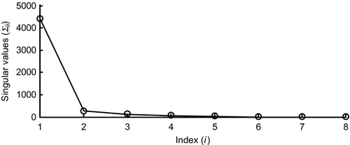
The svd() function does not throw out any of the zero (or near-zero) eigenvalues; this is left to the user. Here, U is an N × M matrix, SIGMA is an M × M diagonal matrix of singular values, and V is an M × M matrix. The diagonal of SIGMA has been copied into the column-vector, sigma, for convenience. A plot of the singular values of the Atlantic Rock data set reveals that the first value is by far the largest, values 2 through 5 are intermediate in size and values 6 through 8 are near-zero. The fact that the first singular value, Σ₁₁, is much larger than all the others reflects the composition of the rock samples having only a small range of variability. Thus, all rock samples contain a large amount of the first factor, f₁—the typical sample. Only five factors, f₁, f₂, f₃, f₄, and f_5, out of a total of eight are needed to describe the samples and their variability about the typical sample requires only four (factors 2 through 5) (Figure 8.3):

The role of each of the factors can be understood by examining its elements. Factor 2, for instance, increases the amount of MgO while decreasing mostly Al₂O₃ and CaO, with respect to the typical sample.

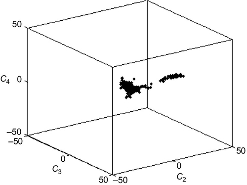
The factor analysis has reduced the dimensions of variability of the rock dataset from 8 elements to 4 factors, improving the effectiveness of scatter plots. MatLab's three-dimensional plotting capabilities are useful in this case, as any three of the four factors can be used as axes and the resulting three-dimensional scatter plot viewed from a variety of perspectives. The following MatLab command plots the coefficients of factors 2 through 4 for each sample:

plot3(C(:,2), C(:,3), C(:,4), ‘k.’);

(MatLab eda08_04)

The plot can then be viewed from different perspectives by using the rotation controls of the figure window (Figure 8.4). Note that the samples appear to form two populations, one in which the variability is due to f₂ and another due to f₃.

8.4 Spiky factors

As mentioned earlier, the factors, F, of a set of samples, S, are nonunique. The equation, S = CF, can always be modified to S = CM⁻¹MF, where M is an arbitrary P × P matrix, defining a new set of factors, F′ = MF. Singular value decomposition is useful because it allows the determination of a set of P ≤ M factors that adequately approximate S. However, it does not always provide the most desirable set of factors. Modifying the set of P factor by using the matrix, M, does not change the value of P or the quality of the fit, but can be used to produce factors with more desirable properties than those produced by singular value decomposition.

One possible guiding principle is the prior information that the factors should be spiky; that is, they should have just a few large elements, with the other elements being near-zero. Minerals, for example, obey this principle. While a rock can contain upward of twenty chemical elements, typically it will be composed of minerals such as fosterite (Mg₂SiO₄), anorthite (CaAl₂Si₂O₈), rutile (TiO₂), etc., each of which contains just a few elements. Spikiness is more or less equivalent to the idea that the elements of the factors should have high variance. The usual formula for the variance, σ_d², of a data set, d, is

${\sigma }_d^2=\frac{1}{N}\left(\sum _{i=1}^N{(d_i-\overline{d})}^2\right)=\frac{1}{N^2}\left(N\sum _{i=1}^N{d}_i^2-{\left(\sum _{i=1}^N{d}_i\right)}^2\right)$

Its generalization to a factor, f_i, is

${\sigma }_f^2=\frac{1}{M^2}\left(M\sum _{i=1}^M{f}_i^4-{\left(\sum _{i=1}^M{f}_i^2\right)}^2\right)$

Note that this is the variance of the squares of the elements of the factors. Thus, a factor, f, has a large variance, σ_f², if the absolute values of its elements have high variation. The signs of the elements are irrelevant.

The varimax procedure is a way of constructing a matrix, M, that increases the variance of the factors while preserving their orthogonality. It is an iterative procedure, with each iteration operating on only one pair of factors, with other pairs being operated upon in subsequent iterations. The idea is to view the factors as vectors, and to rotate them in their plane (Figure 8.5) by an angle, θ, chosen to maximize the sum of their variances. The rotation changes only the two factors, leaving the other P − 2 factors unchanged, as in the following example:

$\left[\begin{array}{c}\hfill {\mathbf{f}}_1^{\text{T}}\hfill \\ \hfill {\mathbf{f}}_2^{\text{T}}\hfill \\ \hfill cos\left(\theta \right){\mathbf{f}}_3^{\text{T}}+sin\left(\theta \right){\mathbf{f}}_5^{\text{T}}\hfill \\ \hfill {\mathbf{f}}_4^{\text{T}}\hfill \\ \hfill -sin\left(\theta \right){\mathbf{f}}_3^{\text{T}}+cos\left(\theta \right){\mathbf{f}}_5^{\text{T}}\hfill \\ \hfill {\mathbf{f}}_6^{\text{T}}\hfill \end{array}\right]=\left[\begin{array}{cccccc}\hfill 1\hfill & \hfill 0\hfill & \hfill 0\hfill & \hfill 0\hfill & \hfill 0\hfill & \hfill 0\hfill \\ \hfill 0\hfill & \hfill 1\hfill & \hfill 0\hfill & \hfill 0\hfill & \hfill 0\hfill & \hfill 0\hfill \\ \hfill 0\hfill & \hfill 0\hfill & \hfill cos\left(\theta \right)\hfill & \hfill 0\hfill & \hfill sin\left(\theta \right)\hfill & \hfill 0\hfill \\ \hfill 0\hfill & \hfill 0\hfill & \hfill 0\hfill & \hfill 1\hfill & \hfill 0\hfill & \hfill 0\hfill \\ \hfill 0\hfill & \hfill 0\hfill & \hfill -sin\left(\theta \right)\hfill & \hfill 0\hfill & \hfill cos\left(\theta \right)\hfill & \hfill 0\hfill \\ \hfill 0\hfill & \hfill 0\hfill & \hfill 0\hfill & \hfill 0\hfill & \hfill 0\hfill & \hfill 1\hfill \end{array}\right]\left[\begin{array}{c}\hfill {\mathbf{f}}_1^{\text{T}}\hfill \\ \hfill {\mathbf{f}}_2^{\text{T}}\hfill \\ \hfill {\mathbf{f}}_3^{\text{T}}\hfill \\ \hfill {\mathbf{f}}_4^{\text{T}}\hfill \\ \hfill {\mathbf{f}}_5^{\text{T}}\hfill \\ \hfill {\mathbf{f}}_6^{\text{T}}\hfill \end{array}\right]\text{or}\mathbf{F}\mathbf{\prime }=\mathbf{MF}$

Here, only the pair, f₃ and f₅, are changed.

In Equation (8.19), the matrix, M, represents a rotation of one pair of vectors. The rotation matrix for many such rotations is just the product of a series of pair-wise rotations. Note that the matrix, M, obeys the rule, M⁻¹ = M^T (that is, M is a unary matrix). For a given pair of factors, f^A and f^B, the rotation angle, θ, is determined by minimizing Φ(θ) = M²(σ_fA² + σ_fB²) with respect to θ (i.e., by solving dΦ/dθ = 0).

The minimization requires a substantial amount of algebraic and trigonometric manipulation, so we omit it here. The result is (Kaiser, 1958) as follows:

$\begin{array}{c}\hfill \theta =\raisebox{1ex}{$1$}\!\left/ \!\raisebox{-1ex}{$4$}\right.{tan}^{-1}\frac{2M\sum _i{u}_i{v}_i-\sum _i{u}_i\sum _i{v}_i}{M\sum _i(u_i^2-v_i^2)-\left({\left(\sum _i{u}_i\right)}^2-{\left(\sum _i{v}_i\right)}^2\right)}\hfill \\ \hfill \text{with}\hfill \\ \hfill u_i={\left(f_i^A\right)}^2-{\left(f_i^B\right)}^2\text{and}{v}_i=2f_i^A{f}_i^B\hfill \end{array}$

By way of example, we note that the two vectors ${\mathbf{f}}^A=\raisebox{1ex}{$1$}\!\left/ \!\raisebox{-1ex}{$2$}\right.{[1,1,1,1]}^{\text{T}}$ and ${\mathbf{f}}^B=\raisebox{1ex}{$1$}\!\left/ \!\raisebox{-1ex}{$2$}\right.{[1,-1,1,-1]}^{\text{T}}$ are extreme examples of two nonspiky orthogonal vectors, because all their elements have the same absolute value. When applied to them, the varimax procedure returns f^A′ = (1/√2)[1, 0, 1, 0]^T and f^B′ = (1/√2) [0, −1, 0, −1]^T, which are significantly spikier than the originals (see MatLab script eda08_05). The MatLab code is as follows:

u = fA.^2 − fB.^2;
v = 2* fA.* fB;
A = 2*M*u'*v;
B = sum(u)*sum(v);
top = A − B;
C = M*(u‘*u−v’*v);
D = (sum(u)^2) − (sum(v)^2);
bot = C − D;
q = 0.25 * atan2(top,bot);
cq = cos(q);
sq = sin(q);
fAp = cq*fA + sq*fB;
fBp = − sq*fA + cq*fB;

(MatLab eda08_05)

See Note 6.1 for a discussion of the atan2() function. Here, the original pair of factors fA and fB, and the rotated pair are fAp and fBp.

We apply this procedure to factors f₂ through f₅ of the Atlantic Rock dataset (that is, the factors related to deviations about the typical rock). The varimax procedure is applied to all pairs of these factors and achieves convergence after several such iterations. The MatLab code for the loops is as follows:

FP = F;
% spike these factors using the varimax procedure
k = [2, 3, 4, 5]′;
Nk = length(k);
for iter = [1:3]
for ii = [1:Nk]
for jj = [ii+1:Nk]
% spike factors i and j
i=k(ii);
j=k(jj);
% copy factors from matrix to vectors
fA = FP(i,:)′;
fB = FP(j,:)′;
% standard varimax procedure to determine rotation angle q
–––
% copy rotated factors back to matrix
FP(i,:) = fAp′;
FP(j,:) = fBp′;
end
end
end

(MatLab eda08_06)

Here the rotated matrix of factors, FP, is initialized to the original matrix of factors, F, and then modified by the varimax procedure (omitted and replaced with a “–––”), with each pass through the inner loop rotating one pair of factors. The procedure converges very rapidly, with three iterations of the outside loop being sufficient.

The resulting factors (Figure 8.6) are much spikier than the original ones. Each now involves mainly variations in one chemical element. For example, f′₂ mostly represents variations in MgO and f′₅ mostly represents variations in Al₂O₃.

8.5 Weighting of elements

An element can be important even though its concentration is extremely low. Gold, for instance, is economic in ore at 5 parts per million and arsenic is unhealthy in drinking water at 10 parts per billion. When a data set contains both high- and low-concentration elements, the procedure described in Section 8.3 for choosing a set of P important factors will lead to an approximation ${\mathbf{S}}_P\approx {\mathbf{S}}^{obs}$ that only poorly describes patterns in the low-concentration elements, because the overall quality of the fit is dominated by the much larger errors of the high-concentration elements.

This problem can be avoided by weighting each element by an amount, say w_i, that reflects its importance. The singular value decomposition is performed on the matrix S^obsW, where W is a diagonal matrix with elements $W_{ii}=w_i$:

${\mathbf{S}}^{obs}\mathbf{W}=\mathbf{U}\mathbf{\Sigma }{\mathbf{V}}^{\mathrm{T}}\mathrm{so}\mathbf{C}={\mathbf{U}}_{\mathrm{P}}{\mathbf{\Sigma }}_{\mathrm{P}}\mathrm{and}\mathbf{F}={{\mathbf{V}}_{\mathrm{P}}}^{\mathrm{T}}{\mathbf{W}}^{-1}$

The weights can be chosen in any of several ways. One possibility is to set them intuitively, to reflect the qualitative importance of each element. Another possibility is to scale them according to the certainty of the measurements; that is, to set $w_i=1/{\sigma }_i$, where σ_i² is the prior variance of the i-th element. This choice leads to each element being fit to similar relative error (Figure 8.7).

8.6 Q-mode factor analysis and spatial clustering

The eigenvectors U and V play completely symmetric roles in the singular value decomposition of the sample matrix S = UΣV^T. We introduced an asymmetry when we grouped them as S = (UΣ)(V^T) = CF, to define the loadings C and factors F.

This grouping is associated with the term R-mode factor analysis. The R-mode factors F = V^T express patterns of variability among elements. Thus, for example, the table in Section 8.3 indicates that the elements in the Atlantic rock dataset contains a pattern, quantified by factor f⁽²⁾, in which Al₂O₃ and MgO are strongly and negatively correlated and another pattern, quantified by factor f⁽³⁾, in which Al₂O₃ and FeO_total are strongly and negatively correlated. These correlations reduce the effective number of elements; that is, they to allow us to substitute a small number of factors for a large number of elements.

Alternately, we could have grouped the singular value decomposition as S = (U)(ΣV^T), an approach associated with the term Q-mode factor analysis. The equivalent transposed form S^T = (VΣ)(U^T) is more frequently encountered in the literature, and is also more easily understood, since it can be interpreted as ‘normal factor analysis’ applied to the matrix S^T. The transposition has reversed the sense of samples and elements, so the Q-mode factors F = U^T quantify patterns of variability among samples, in the same way that the R-mode V^T quantifies patterns of variability among elements.

The sampling in the Atlantic rock dataset is geographical, so the Q-mode factors express patterns of spatial variability and can be used to detect geographical clustering. These spatial patterns can be brought out by plotting the components of each factor on a map, with the i-th component plotted at the location of sample i and with its numberial value depicted by the color (or grey shade) or the symbo. When applied to the Atlantic rock datset, this technique demonstrated that that the chemistry of the mid-Atlantic ridge (north-south bands of symbols in Figure 8.8) is strongly segmented, with $~10$ degree long sections of failry uniform chemistry punctuated by spatially-sharp jumps.

8.7 Time-Variable functions

The samples in the Atlantic Rock dataset do not appear to have an intrinsically-meaningful order. As far as we know, their order in the file could merely reflect the order that the samples were entered into the database by the personnel who compiled the data set. However, one might imagine a similar dataset in which sample order is significant. One example would be a set of chemical analyses made in the same place as a sequence of times. The time sequence could be used to characterize the chemical evolution of the system. Sample, s⁽ⁱ⁾, quantifies the chemical composition at time, t_i.

The ordering of the elements in the Atlantic Rock dataset does not appear to have any special significance either. It does not reflect their abundance in a typical rock. It is not even alphabetical. However, one might imagine a similar dataset in which the order of chemical constituents is significant. One example would be a set of analyses of the concentration of alkanes (methane (CH₄), ethane (C₂H₈), propane (C₃H₈), etc.) in a hydrocarbon mixture, as the chemical properties of these carbon-chain molecules are critically dependent on the number of carbon atoms in the chain. In this case, ordering the elements by the increasing length, x, of the carbon chain would be appropriate. The standard equation for factors (Equation 8.2) could then be interpreted in terms of variation in x and t:

${\mathbf{s}}^{\left(i\right)}=\sum _{k=1}^P{C}_{\mathrm{ki}}{\mathbf{f}}^{\left(k\right)}\text{or}s(x_j,t_i)=\sum _{k=1}^P{C}_k\left(t_i\right)f_k\left(x_j\right)$

Note that the analysis has broken out the (x, t) dependence into dependence on, x and t, separately. The factors, f_k(x_j), each describe a pattern in x and the factor loadings, C_k(t_i), describe the temporal, t, variation of those patterns. When used in this context, the factors are called empirical orthogonal functions, or EOFs. In the hydrocarbon example, above, a plot of the elements of a factor, f_k(x), against x would display the distribution of alkane chain length within the k-th factor. A plot of C_k(t) against time, t, would display the time-dependent amplitude the k-th factor. One might imagine a chemical evolution process in which chain length of alkanes decreased systematically with time. This behavior would be manifested in a temporal evolution of the factor loadings, with the mix becoming increasingly rich in those factors that contained larger fractions of short-length alkanes.

A sample is just a collection of numbers arranged in column vector format. While the alkane data set has a one-dimensional organization that makes the use of vectors natural, a one-dimensional organization is not required by the factor analysis method. Samples could, for instance, have the natural organization of a two-dimensional or three-dimensional grid. The grid merely would need to be rearranged into a vector for the method to be applied (see Section 5.9).

The Climate Analysis Center (CAC) Equatorial Pacific Ocean Sea Surface Temperature data set is one such example. It is a time sequence of two-dimensional grids of the surface temperature of a patch of the equatorial Pacific Ocean, a part of the world important to the study of the El Niño/La Niña climate oscillation. Bill Menke, who retrieved the data, provides the following report:

A 6-year portion of the CAC dataset is shown (Figure 8.9). Many of the monthly images show an east-west band of cold (white) temperatures that is characteristic of the La Niña phase of the oscillation. A few (e.g., late 1972) show a warm (black) band, most prominent in the eastern Pacific that is characteristic of the El Niño phase.

The CAC data set comprises N = 399 monthly images, each with M = 2520 grid points (30 in latitude, 84 in longitude). Each factor (or empirical orthogonal function, EOF) is a 2520-length vector that folds into a 30 × 84 spatial grid of temperature values. The total number of EOFs is M = 399, but as is shown in Figure 8.10, many have exceedingly small singular values and can be discarded. As the data represent a temperature anomaly (that is, temperature minus its mean value), the first EOF will not resemble the mean temperature, but rather will characterize the maximum amplitude spatial variation. A visual inspection (Figure 8.11) reveals that it consists of an east-west cold (white) band crossing the equatorial region and is thus a La Niña pattern.

Plots of the factor loadings, the time-dependent amplitude of the EOFs, indicate that the first five factors have time-variation with significant power at periods greater than 1 year (Figure 8.12). The coefficient of the first EOF is essentially a La Niña index, as the shape of the first EOF is diagnostic of La Niña conditions. Peaks in it indicate times when the La Niña pattern is particularly strong, and troughs indicate when it is particularly weak. The El Niño years of 1972, 1983, and 1997 show up as prominent troughs in this time series.

The EOFs can be used as a method of smoothing the temperature data in a way that preserves the most important spatial and temporal variations. A reconstruction using just the first five EOFs is shown in Figure 8.13.

Problems

8.1. Write the matrix, SS^T, in terms of U, V, and Σ and show that the columns of U are eigenvectors of SS^T.

8.2. The varimax procedure uses one type of prior information, spikiness, to build a set of P “improved” factors, f′_i, out of the set of P significant factors, f_i, computed using singular value decomposition. Another, different type of prior information is that the factors, f′_i, are close in shape to some other set of P factors, f_i^s, that are specified. Find linear mixtures of the factors, f_i, computed using singular value decomposition that comes as close as possible to f_i^s, in the sense of minimizing, Σ_i (f′_i − f_i^s) (f′_i − f_i^s)^T.

8.3. Compute the power spectra of each of the EOF amplitude (factor loading) time series for the CAC dataset. Which one has the most power at a period of exactly 1 year? Describe and interpret the spatial pattern of the corresponding EOF.

8.4. Cut the Black Rock Forest temperature dataset up into a series of one-day segments.
Discard any segments that contain hot or cold spikes or data dropouts. Subtract out the mean of each segment so that they reflect only the temperature changes through the course of the day, and not the seasonal cycle of temperatures. Consider each segment a sample and analyze the dataset with empirical orthogonal function analysis, making and interpreting plots that are analogous to Figure 8.9-8.13.

8.5. Invent a scenario in which the factor loadings (amplitudes of EOF's) are a function of two spatial coordinates, (x, y) instead of time, t, and in which they could be used to solve a nontrivial problem.