9.1 Correlation is covariance

When we create a scatter plot of observations, we are treating the data as random variables. The underlying idea is that two data types (or elements), say d_i and d_j, are scattering about their typical values. Sometimes the scatter is due to measurement noise. Sometimes it is due to an unmodeled natural process that we can only treat probabilistically. But in either case, we are viewing the cloud of data points as being drawn from a joint probability density function, p(d_i, d_j). The data are correlated if the covariance of this function is nonzero. Thus, the covariance matrix, C, is extremely useful in quantifying the degree to which different elements correlate. Recall that the covariance matrix associated with p(d_i, d_j) are defined as:

$C_{ij}={\displaystyle {\int }_{-\infty }^{+\infty }{\displaystyle {\int }_{-\infty }^{+\infty }(d_i-{\overline{d}}_i)(d_j-{\overline{d}}_j)p(d_i,d_j)\text{d}{d}_i\text{d}{d}_j}}$

Here ${\overline{d}}_i$ and ${\overline{d}}_j$ are the means of d_i and d_j, respectively. We can estimate C_ij from a data set by approximating the probability density function with a histogram constructed from the observed data. We first divide the (d_i, d_j) plane into many small bins, numbered by the index s. Each bin has area Δd_iΔd_j and is centered at (d_i^(s), d_j^(s)) (Figure 9.1). We now denote the number of data pairs in bin s by N_s. The probability, p(d_i, d_j) Δd_iΔd_j ≈ N_s/N, where N is the total number of data pairs, so

$C_{ij}\approx \frac{1}{N}{\displaystyle \sum _s[d_i^{(s)}-{\overline{d}}_i][d_j^{\left(s\right)}-{\overline{d}}_j]N_s}$

We now shrink the size of the patches so that at most one data pair is in each bin. Then, N_s equals either zero or unity. Summation over the patches is equal to summation over the (d_i, d_j) pairs themselves:

$C_{ij}\approx \frac{1}{N}{\displaystyle \sum _{k=1}^N[d_i^{(k)}-{\overline{d}}_i^{}][d_j^{\left(k\right)}-{\overline{d}}_j^{}]}$

The covariance is nonzero when the data exhibit some degree of correlation, but its actual numerical value depends on the overall range of the data. The range can be normalized to ±1 by scaling by the square root of the product of variances:

$R_{ij}=\frac{C_{ij}}{\sqrt{C_{ii}{C}_{jj}}}$

The quantity R is called the matrix of correlation coefficients, and its elements are called correlation coefficients and are denoted by the lower-case letter, r. When, as above, they are estimated from the data (as contrasted to being computed from the probability density function), they are referred to as sample correlation coefficients. See Table 9.1 for a list of important quantities, such as R, that are introduced in this chapter. The covariance, C, and correlation coefficient matrix, R, can be estimated from a set of data, D, as follows:

Table 9.1

Important Quantities Used in Chapter 9.

Symbol	Name	Created from	Significance
Cd	Covariance matrix of the data, d	Probability density function of the data, p(d)	Diagonal elements, [Cd]ij with i = j: variance of the data, di; squared width of the univariate probability density function, p(di) off-diagonal elements, [Cd]ij with i ≠ j: degree of correlation between the pair of observations, di and dj
R	Matrix of correlation coefficients	Probability density function of the data, p(d)	Normalized version of Cd with elements that vary between ±1 elements of R given the symbol, r
$\mathbf{a}=\mathbf{d}\star \mathbf{d}$	Autocorrelaton function	Time series, d	Element ak: degree of correlation between two elements of d separated by a time lag, τ = (k − 1)Δt
$\mathbf{c}={\mathbf{d}}^{\left(1\right)}\star {\mathbf{d}}^{\left(2\right)}$	Cross-correlation function	Two time series, d(1) and d(2)	Element ck: degree of correlation between an element of d(1) and an element of d(2) separated by a time lag, τ = (k − 1)Δt
$\mathbf{f}*\mathbf{d}$	Convolution	Filter, f, and time series, d	Filters the times series, d, with the filter, f
$\tilde{d}(\omega )$	Fourier transform	Time series, d(t)	Amplitude of sines and cosines of frequency, ω, in the time series
C2(ω0, Δω)	Coherence	Two time series, d(1) and d(2)	Similarity between d(1) and d(2) at frequencies in the range, ω0 ± Δω varies between 0 and 1

C = cov(D); % covariance
R = corrcoef(D); % correlation coefficient

(MatLab eda09_01)

Here, D, is an N × M matrix organized so that D_ij is the amount of element, j, in sample i (the same arrangement as in Equation 8.1). The matrix, R, is M × M, so that R_ij expresses the degree of correlation of elements i and j. Figure 9.2A depicts the matrix of correlation coefficients for the Atlantic rock dataset, in which the elements are literal chemical elements. The diagonal elements are all unity, as a data type correlates perfectly with itself. Some pairs of chemical components, such as TiO₂ and NaO₂, strongly correlate with each other (Figure 9.2B). Other pairs, such as TiO₂ and Al₂O₃, are nearly uncorrelated.

The idea of correlation can also be applied to the elements of a time series. Neighboring samples in a time series are often highly correlated (and hence predictable), even though the time series as a whole may be random. Consider, for example, the stream flow of the Neuse River. On the one hand, a hydrologist, working a year ago, would not have been able to predict whether today’s discharge is unusually high or low. It is just not possible to predict individual storms—the source of the river’s water—a year in advance; they are best considered random phenomena. On the other hand, if today’s discharge is high, the chances are excellent that tomorrow’s discharge will be high as well. Stream flow persists for a few days, because the rain water takes time to drain away.

The notion of short term correlation within the stream flow time series can also be described by a joint probability density function. If we denote the river’s discharge at time t_i as d_i, and discharge at time t_j as d_j, then we can speak of the joint probability density function p(d_i, d_j). In the case of stream flow, we expect that d_i and d_j will have a strong positive correlation when the time difference or lag, τ = t_i − t_j, is small (Figure 9.3A). When the measurements are more widely separated in time, then we expect the correlation to be weaker (Figure 9.3B). We expect discharge to be uncorrelated at separations of, say, a month or so (Figure 9.3C). On the other hand, discharge will again be positively correlated, although maybe only weakly so, at separations of about a year, because patterns of stream flow have an annual cycle. Note that we must assume that the time series is stationary, meaning that its statistical properties do not change with time, or else the degree of correlation would depend on the measurement times, as well as the time difference between them.

We already have the methodology to quantify the degree of correlation of a joint probability density function: its covariance matrix, C_ij. In this case, we manipulate the formula to bring out the means, because in many cases we will be dealing with time series that fluctuate around zero:

$\begin{array}{l}{C}_{ij}={\displaystyle {\int }_{-\infty }^{+\infty }{\displaystyle {\int }_{-\infty }^{+\infty }(d_i-\overline{d})(d_j-\overline{d})p(d_i,d_j)\text{d}{d}_i\text{d}{d}_j}}\hfill \\ ={\displaystyle {\int }_{-\infty }^{+\infty }{\displaystyle {\int }_{-\infty }^{+\infty }{d}_i{d}_{j}p(d_i,d_j)\text{d}{d}_i\text{d}{d}_j}-2{\overline{d}}^2+{\overline{d}}^2=A_{ij}-{\overline{d}}^2}\hfill \\ \text{with}{A}_{ij}={\displaystyle {\int }_{-\infty }^{+\infty }{\displaystyle {\int }_{-\infty }^{+\infty }{d}_i{d}_{j}p(d_i,d_j)\text{d}{d}_i\text{d}{d}_j}}\hfill \end{array}$

Here, the mean, $\overline{d}$, of the time series is assumed to be independent of time (so it has no index). The matrix, A, is called the autocorrelation matrix of the time series. It is equal to the covariance matrix when the mean of the time series is zero.

Just as in the case of the covariance, the autocorrelation can be estimated from observations. The data are pairs of samples drawn from the time series, where one member of the pair is lagged by a fixed time interval, τ = (k − 1)Δt, with respect to the other (with k an integer; note that k = 1 corresponds to τ = 0). A time series of length N has N − |k − 1| such pairs. We then form a histogram of the pairs, as we did in the case of covariance, so that the integral in Equation (9.5) can be approximated by a summation:

$A_{i,j}={\int }_{-\infty }^{+\infty }{\int }_{-\infty }^{+\infty }{d}_i{d}_{j}p(d_i,d_j)\text{d}{d}_i\text{d}{d}_j\approx \frac{1}{N-\left|k-1\right|}\sum _s{d}_i^{(s)}{d}_j^{(s)}{N}_s.$

Once again, we shrink the size of the bins so that at most one pair is in each bin and N_s equals either zero or unity, so summation over the bin is equal to summation over the data pairs themselves. For the k > 0 case, we have

$\begin{array}{l}\hfill A_{i,k+i-1}\approx \frac{1}{N-\left|k-1\right|}{\displaystyle \sum _s{d}_i^{\left(s\right)}{d}_{k+i-1}^{\left(s\right)}{N}_s}=\frac{1}{N-\left|k-1\right|}{\displaystyle \sum _{i=1}^{N-k+1}{d}_i{d}_{k+i-1}}=\frac{a_k}{N-\left|k-1\right|}\hfill \\ \hfill \text{with}{a}_k={\displaystyle \sum _{i=1}^{N-k+1}{d}_i{d}_{k+i-1}}\text{and}k>0\hfill \end{array}$

The column vector, a, is called the autocorrelation of the time series. An element, a_k, is called the autocorrelation at time lag, τ = k − 1. The autocorrelation at negative lags equals the autocorrelation at positive lags, as A is a symmetric matrix, that is, A_ij = a_k, with k = |i − j| + 1. As we have defined it above, a_k is unnormalized, in the sense that it omits the factor of 1/(N − |k − 1|).

In MatLab, the autocorrelation is calculated as follows:

a = xcorr(d);

(MatLab Script eda09_03)

Here, d is a time series of length N. The xcorr() function returns a vector of length 2N − 1 that includes both negative and positive lags so that the zero lag element is a(N).

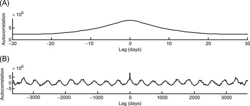
The autocorrelation of the Neuse River hydrograph is shown in Figure 9.4. For small lags, say of less than a month, the autocorrelation falls off rapidly with lag, with a time scale that reflects the time that rain water needs to drain away after a storm. For larger lags, say of a few years, the autocorrelation oscillates around zero with a period of one year. This behavior reflects the seasonal cycle. Summer and winter discharges are negatively correlated, as one tends to be high when the other is low.

9.2 Computing autocorrelation by hand

The autocorrelation at zero lag (k = 1) can be calculated by hand by writing down two copies of the time series, one above the other, multiplying adjacent terms, and adding:

$\begin{array}{c}\hfill \begin{array}{ccccc}\hfill d_1\hfill & \hfill d_2\hfill & \hfill d_3\hfill & \hfill \cdots \hfill & \hfill d_N\hfill \\ \hfill d_1\hfill & \hfill d_2\hfill & \hfill d_3\hfill & \hfill \cdots \hfill & \hfill d_N\hfill \\ \hfill \times \hfill & \hfill \hfill & \hfill \hfill & \hfill \hfill & \hfill \hfill \\ \hfill d_1^2\hfill & \hfill d_2^2\hfill & \hfill d_3^2\hfill & \hfill d_N^2\hfill & \hfill d_N^2\hfill \end{array}\hfill \end{array}\stackrel{\text{yields}}{\to }{a}_1=d_1^2+d_2^2+d_3^2+\cdots +d_N^2$

Note that a₁ is proportional to the power in the time series. Subsequent elements of a_k are calculated by progressively offsetting one copy of the time series with respect to the other, prior to multiplying and adding (and ignoring the elements with no overlap). The lag Δt (k = 2) element is as follows:

$\begin{array}{c}\hfill \begin{array}{cccccc}\hfill d_1\hfill & \hfill d_2\hfill & \hfill d_3\hfill & \hfill \cdots \hfill & \hfill d_N\hfill & \hfill \hfill \\ \hfill \hfill & \hfill d_1\hfill & \hfill d_2\hfill & \hfill \cdots \hfill & \hfill d_{N-1}\hfill & \hfill d_N\hfill \\ \hfill \times \hfill & \hfill \hfill & \hfill \hfill & \hfill \hfill & \hfill \hfill & \hfill \hfill \\ \hfill \hfill & \hfill d_2{d}_1\hfill & \hfill d_3{d}_2\hfill & \hfill \cdots \hfill & \hfill d_N{d}_{N-1}\hfill & \hfill \hfill & \hfill \hfill \end{array}\hfill \end{array}\stackrel{\text{yields}}{\to }{a}_2=d_2{d}_1+d_3{d}_2+d_4{d}_3+\cdots +d_N{d}_{N-1}$

and the lag 2Δt (k = 3) element is as follows:

$\begin{array}{c}\hfill \begin{array}{cccccccc}\hfill d_1\hfill & \hfill d_2\hfill & \hfill d_3\hfill & \hfill d_4\hfill & \hfill \cdots \hfill & \hfill d_N\hfill & \hfill \hfill & \hfill \hfill \\ \hfill \hfill & \hfill \hfill & \hfill d_1\hfill & \hfill d_2\hfill & \hfill \cdots \hfill & \hfill d_{N-2}\hfill & \hfill d_{N-1}\hfill & \hfill d_N\hfill \\ \hfill \times \hfill & \hfill \hfill & \hfill \hfill & \hfill \hfill & \hfill \hfill & \hfill \hfill & \hfill \hfill & \hfill \hfill \\ \hfill \hfill & \hfill \hfill & \hfill d_1{d}_3\hfill & \hfill d_2{d}_4\hfill & \hfill \cdots \hfill & \hfill d_{N-2}{d}_N\hfill & \hfill \hfill & \hfill \hfill & \hfill \hfill \end{array}\hfill \end{array}\stackrel{\text{yields}}{\to }{a}_3=d_1{d}_3+d_2{d}_4+\cdots +d_{N-2}{d}_N$

9.3 Relationship to convolution and power spectral density

The formula for the autocorrelation is very similar to the formula for the convolution (Equation 7.1):

$\begin{array}{cccc}\hfill \text{autocorrelation}\hfill & \hfill \hfill & \hfill \hfill & \hfill \text{convolution}\hfill \\ \hfill a_k={\displaystyle \sum _i{d}_i{d}_{k+i-1}}\hfill & \hfill \hfill & \hfill \hfill & \hfill {\theta }_k={\displaystyle \sum _i{g}_i{h}_{k-i+1}}\hfill \\ \hfill \hfill & \hfill \hfill \\ \hfill \hfill & \hfill \hfill \\ \hfill a\left(t\right)={\displaystyle {\int }_{-\infty }^{+\infty }d\left(\tau \right)d(t+\tau )\text{d}\tau }\hfill & \hfill \hfill & \hfill \hfill & \hfill \theta \left(t\right)={\displaystyle {\int }_{-\infty }^{+\infty }g\left(\tau \right)h(t-\tau )\text{d}\tau }\hfill \\ \hfill a=d\star d\hfill & \hfill \hfill & \hfill \hfill & \hfill \theta =g*h\hfill \end{array}$

Note that a five pointed star, , is used to indicate autocorrelation, in the same sense that an asterisk, *, is used to indicate convolution. The two formulas are very similar, except that in the case of the convolution, one of the two time series is backward in time, in contrast to the autocorrelation, where both are forward in time. The relationship between the two can be found by transforming the autocorrelation integral to a new variable, τ′ = −τ,

$a\left(t\right)=d\left(t\right)\star d\left(t\right)={\int }_{-\infty }^{+\infty }d\left(\tau \right)d(t+\tau )\text{d}\tau ={\int }_{-\infty }^{+\infty }d(-\tau \prime )d(t-\tau )\text{d}\tau \prime =d(-t)*d\left(t\right)$

Thus, the autocorrelation is the convolution of a time-reversed time series with the original time series.

Two neighboring points on a time series will correlate strongly with each other if the time series varies slowly between them. A time series with an autocorrelation that declines slowly with lag is necessarily richer in low frequency energy than one that declines quickly with lag. This relationship can be explored by computing the Fourier transform of the autocorrelation. The calculation is simplified by recalling that the Fourier transform of a convolution is the product of the transforms. Thus,

$\tilde{a}\left(\omega \right)=ℱ\left\{d(-t)\right\}\tilde{d}\left(\omega \right)$

where $ℱ${−d(t)} stands for the Fourier transform of d(−t). We compute it as follows:

$ℱ\left\{d(-t)\right\}={\displaystyle {\int }_{-\infty }^{+\infty }d(-t)exp\left(\text{i}\omega t\right)\text{d}t}{\displaystyle {\int }_{-\infty }^{+\infty }d(t\prime )exp\left(\text{i}\right(-\omega )t\prime )\text{d}t\prime }=\tilde{d}(-\omega )={\tilde{d}}^{*}(\omega )$

Here, we have used the transformation of variables, t′ = −t, together with the fact that, for real time series, $\tilde{d}(\omega )$ and $\tilde{d}(-\omega )$ are complex conjugates of each other. Thus,

$\tilde{a}(\omega )={\tilde{d}}^{*}(\omega )\tilde{d}(\omega )={\left|\tilde{d}(\omega )\right|}^2$

The Fourier transform of the autocorrelation is proportional to the power spectral density of the time series. As we have seen in Section 6.5, functions that are broad in time have Fourier transforms that are narrow in frequency. Hence, a time series with a broad autocorrelation function has most of its power at low frequencies.

9.4 Cross-correlation

The underlying idea behind the autocorrelation is that pairs of samples drawn from the same time series, and separated by a fixed time lag, τ, are correlated. This idea can be generalized to pairs of samples drawn from two different time series. As an example, consider time series of precipitation, u, and stream flow, v. At times when precipitation is high, we expect stream flow to be high, too. However, the time of peak stream flow will be delayed with respect to the time of maximum precipitation, as water takes time to drain from the land. Thus, the precipitation and stream flow time series will be most correlated when the former is lagged by a specific amount of time with respect to the latter.

We quantify this idea by defining the probability density function, p(u_i, v_j), the joint probability for the i-th sample of time series, u, and the j-th sample of time series, v. The autocorrelation then generalizes to the cross-correlation, c_k (written side-by-size with the convolution, for comparison):

$\begin{array}{cc}\hfill \text{cross}-\text{correlation}\hfill & \hfill \text{convolution}\hfill \\ \hfill c_k={\displaystyle \sum _i{u}_i{v}_{k+i-1}}\hfill & \hfill {\theta }_k={\displaystyle \sum _i{g}_i{h}_{k-i+1}}\hfill \\ \hfill \hfill & \hfill \hfill \\ \hfill \hfill & \hfill \hfill \\ \hfill c\left(t\right)={\displaystyle {\int }_{-\infty }^{+\infty }u\left(\tau \right)v(t+\tau )\text{d}\tau }\hfill & \hfill \theta \left(t\right)={\displaystyle {\int }_{-\infty }^{+\infty }g\left(\tau \right)h(t-\tau )\text{d}\tau }\hfill \\ \hfill c=u\star v\hfill & \hfill \theta =g*h\hfill \end{array}$

Note that the five pointed star is used to indicate cross-correlation, as well as autocorrelation, as the autocorrelation of a time series is its cross-correlation with itself. Here, u(t_i) and v(t_i) are two time series, each of length, N. The cross-correlation is related to the convolution by

$c\left(t\right)=u\left(t\right)\star v\left(t\right)=u(-t)*v\left(t\right)$

In MatLab, the cross-correlation is calculated with the function

c = xcorr(u,v);

(MatLab Script eda09_04)

Here, u and v are time series of length, N. The xcorr() function returns both negative and positive lags and is of length, 2N−1. The zero-lag element is c(N). Unlike the autocorrelation, the cross-correlation is not symmetric in lag. Instead, the cross-correlation of v and u is the time-reversed version of the cross-correlation of u and v. Mistakes in ordering the arguments of the xcorr() function will lead to a result that is backwards in time; that is, if u(t) v(t) = c(t), then v(t) u(t) = c(−t).

We note here that the Fourier Transform of the cross-correlation is called the cross-spectral density:

$\tilde{c}\left(\omega \right)={\tilde{u}}^{*}\left(\omega \right)\tilde{v}\left(\omega \right)$

However, we will put off discussion of its uses until Section 9.9.

9.5 Using the cross-correlation to align time series

The cross-correlation is useful in aligning two time series, one of which is delayed with respect to the other, as its peak occurs at the lag at which the two time series are best correlated, that is, the lag at which they best line up. In MatLab,

c = xcorr(u,v);
[cmax, icmax] = max(c);
tlag = −Dt * (icmax−N);

(MatLab eda09_04)

Here, Dt is the sampling interval of the time series and tlag is the time lag between the two time series. The lag is positive when features in v occur at later times than corresponding features in u. This technique is illustrated in Figure 9.5.

We apply this technique to an air quality dataset, in which the objective is to understand the diurnal fluctuations of ozone (O₃). Ozone is a highly reactive gas that occurs in small (parts per billion) concentrations in the earth’s atmosphere. Ozone in the stratosphere plays an important role in shielding the earth’s surface from ultraviolet (UV) light from the sun, for it is a strong UV absorber. But its presence in the troposphere at ground level is problematical. It is a major ingredient in smog and a health risk, increasing susceptibility to respiratory diseases. Tropospheric ozone has several sources, including chemical reactions between oxides of nitrogen and volatile organic compounds in the presence of sunlight and high temperatures. We thus focus on the relationship between ozone concentration and the intensity of sunlight (that is, of solar radiation). Bill Menke provides the following information about the dataset:

The solar radiation and ozone concentration data are shown in Figure 9.6. Both show a pronounced diurnal periodicity, but the peaks in ozone are delayed several hours behind the peaks in sunlight. The lag, determined by cross-correlating the two time series, is 3 h (Figure 9.7). Notice that excellent results are achieved, even though the two dataset do not exactly match.

9.6 Least squares estimation of filters

In Section 7.1, we showed that the convolution equation, g(t)*m(t) = d(t), can be written as a matrix equation of the form, Gm = d, where m and d are the time series versions of m(t) and d(t), respectively, and G is the matrix:

$\mathbf{G}=\left[\begin{array}{ccccc}\hfill g_1\hfill & \hfill 0\hfill & \hfill 0\hfill & \hfill \cdots \hfill & \hfill 0\hfill \\ \hfill g_2\hfill & \hfill g_1\hfill & \hfill 0\hfill & \hfill \cdots \hfill & \hfill 0\hfill \\ \hfill g_3\hfill & \hfill g_2\hfill & \hfill g_1\hfill & \hfill \cdots \hfill & \hfill 0\hfill \\ \hfill \cdots \hfill & \hfill \cdots \hfill & \hfill \cdots \hfill & \hfill \cdots \hfill & \hfill 0\hfill \\ \hfill g_N\hfill & \hfill g_{N-1}\hfill & \hfill g_{N-2}\hfill & \hfill \cdots \hfill & \hfill g_1\hfill \end{array}\right]$

The least squares solution involves the matrix products, G^TG and G^Td:

$\begin{array}{l}{\mathbf{G}}^{\mathbf{T}}\mathbf{G}=\left[\begin{array}{ccccc}\hfill g_1\hfill & \hfill g_2\hfill & \hfill g_3\hfill & \hfill \cdots \hfill & \hfill g_N\hfill \\ \hfill 0\hfill & \hfill g_1\hfill & \hfill g_2\hfill & \hfill \cdots \hfill & \hfill g_{N-1}\hfill \\ \hfill 0\hfill & \hfill 0\hfill & \hfill g_1\hfill & \hfill \cdots \hfill & \hfill g_{N-2}\hfill \\ \hfill \cdots \hfill & \hfill \cdots \hfill & \hfill \cdots \hfill & \hfill \cdots \hfill & \hfill 0\hfill \\ \hfill 0\hfill & \hfill 0\hfill & \hfill 0\hfill & \hfill \cdots \hfill & \hfill g_1\hfill \end{array}\right]\left[\begin{array}{ccccc}\hfill g_1\hfill & \hfill 0\hfill & \hfill 0\hfill & \hfill \cdots \hfill & \hfill 0\hfill \\ \hfill g_2\hfill & \hfill g_1\hfill & \hfill 0\hfill & \hfill \cdots \hfill & \hfill 0\hfill \\ \hfill g_3\hfill & \hfill g_2\hfill & \hfill g_1\hfill & \hfill \cdots \hfill & \hfill 0\hfill \\ \hfill \cdots \hfill & \hfill \cdots \hfill & \hfill \cdots \hfill & \hfill \cdots \hfill & \hfill 0\hfill \\ \hfill g_N\hfill & \hfill g_{N-1}\hfill & \hfill g_{N-2}\hfill & \hfill \cdots \hfill & \hfill g_1\hfill \end{array}\right]\approx \left[\begin{array}{ccccc}\hfill a_1\hfill & \hfill a_2\hfill & \hfill a_3\hfill & \hfill \cdots \hfill & \hfill a_N\hfill \\ \hfill a_2\hfill & \hfill a_1\hfill & \hfill a_2\hfill & \hfill \cdots \hfill & \hfill \cdots \hfill \\ \hfill a_3\hfill & \hfill a_2\hfill & \hfill a_1\hfill & \hfill \cdots \hfill & \hfill \cdots \hfill \\ \hfill \cdots \hfill & \hfill \cdots \hfill & \hfill \cdots \hfill & \hfill \cdots \hfill & \hfill \cdots \hfill \\ \hfill a_N\hfill & \hfill \cdots \hfill & \hfill \cdots \hfill & \hfill \cdots \hfill & \hfill a_1\hfill \end{array}\right]\propto \mathbf{A}\hfill \\ {\mathbf{G}}^{\mathbf{T}}\mathbf{d}=\left[\begin{array}{ccccc}\hfill g_1\hfill & \hfill g_2\hfill & \hfill g_3\hfill & \hfill \cdots \hfill & \hfill g_N\hfill \\ \hfill 0\hfill & \hfill g_1\hfill & \hfill g_2\hfill & \hfill \cdots \hfill & \hfill g_{N-1}\hfill \\ \hfill 0\hfill & \hfill 0\hfill & \hfill g_1\hfill & \hfill \cdots \hfill & \hfill g_{N-2}\hfill \\ \hfill \cdots \hfill & \hfill \cdots \hfill & \hfill \cdots \hfill & \hfill \cdots \hfill & \hfill 0\hfill \\ \hfill 0\hfill & \hfill 0\hfill & \hfill 0\hfill & \hfill \cdots \hfill & \hfill g_1\hfill \end{array}\right]\left[\begin{array}{c}\hfill d_1\hfill \\ \hfill d_2\hfill \\ \hfill d_3\hfill \\ \hfill \cdots \hfill \\ \hfill d_N\hfill \end{array}\right]=\left[\begin{array}{c}\hfill c_1\hfill \\ \hfill c_2\hfill \\ \hfill c_3\hfill \\ \hfill \cdots \hfill \\ \hfill c_N\hfill \end{array}\right]=\mathbf{c}\hfill \end{array}$

Thus, the elements of G^Td are the cross-correlation, c, of the time series d and g and the elements of G^TG are approximately the autocorrelation matrix, A, of the time series, g. The matrix, G^TG, is approximately Toeplitz, with elements [G^TG]_ij = a_k, where k = |i − j| + 1. This result is only approximate, because on close examination, elements that appear to refer to the same autocorrelation are actually different from one another. Thus, for example, [G^TG]₁₁ is exactly a₁, but [G^TG]₂₂ is not, as it is the autocorrelation of the first N − 1 elements of g, not of all of g. The difference grows towards the bottom-right of the matrix.

This technique is sometimes used to solve the filter estimation problem, that is, solve θ = g * h for an estimate of h. We examined this problem previously in Section 7.3, using MatLab script eda07_03. We provide here an alternate version of this script. A major modification is made to the function called by the biconjugate gradient solver, bicg(). It now uses the autocorrelation to perform the multiplication F^TFv. The function was previously called filterfun() but is renamed here to autofun():

function y = autofun(v,transp_flag)
global a H;
N = length(v);
% FT F v = GT G v + HT H v
GTGv=zeros(N,1);
for i = [1:N]
 GTGv(i) = [fliplr(a(1:i)′), a(2:N−i+1)′] * v;
 end
Hv = H*v;
HTHv = H′*Hv;
y = GTGv + HTHv;
return

(MatLab autofun)

The global variable, a, contains the autocorrelation of g. It is computed only once, in the main script. The main script also performs the cross-correlation prior to the call to bicg():

clear a H;
global a H;
–––
al = xcorr(g);
Na = length(al);
a = al((Na+1)/2: Na);
–––
cl = xcorr(qobs2, g);
Nc = length(cl);
c = cl((Nc+1)/2: Nc);
–––
% set up F′f = GT qobs + HT h
% GT qobs is c=qobs2*g
HTh = H′* h;
FTf = c + HTh;
% solve
hest3 = bicg(@autofun, FTf, 1e−10, 3*L);

(MatLab eda09_06)

The results, shown in Figure 9.8, can be compared to those in Figure 7.7. The method does a good job recovering the two peaks in h, but suffers from “edge effects,” that is, putting spurious oscillations at the beginning and end of the time series.

9.7 The effect of smoothing on time series

As was discussed in Section 4.5, the smoothing of data is a linear process of the form, d^smooth = Gd^obs. Smoothing is also a type of filtering, as can be seen by examining the form of data kernel, G (Equation 4.16), which is Toeplitz. The columns of G define a smoothing filter, s. Usually, we will want the smoothing to be symmetric, so that the smoothed data, d_i^smooth, is calculated through a weighted average of the observed data, d_j^obs, both to its left and right of i (where j > i corresponds to the future and j < i corresponds to the past). The filter, s_i, is, therefore, noncausal with coefficients that are symmetric about the present value (i = 1). The coefficients need to sum to unity, to preserve the overall amplitude of the data. These traits are exemplified in the three-point smoothing filter (see Equation 4.15):

$\mathbf{s}={[s_0,s_1,s_2]}^{\text{T}}=[¼,½,¼]{}^{\text{T}}$

It uses the present (element, i), the past (element, i − 1) and the future (element, i + 1) of d^obs to calculate d_i^smooth:

$\begin{array}{c}\hfill \text{smoothed data}=\text{weighted average of observed data}\hfill \\ \hfill \text{or}\hfill \\ \hfill d_i^{\text{smooth}}=¼d_{i-1}^{\text{obs}}+½d_i^{\text{obs}}+¼d_{i+1}^{\text{obs}}\hfill \end{array}$

As long as the filter is of finite length, L, we can view the output as delayed with respect to the input, and the filtering operation itself to be causal:

$d_i^{\text{smoothed and delayed}}=¼d_i^{\text{obs}}+½d_{i-1}^{\text{obs}}+¼d_{i-2}^{\text{obs}}$

In this case, the delay is one sample. In general, the delay is (L − 1)/2 samples. The length, L, controls the smoothness of the filter, with large Ls corresponding to large degrees of smoothing (Figure 9.9).

The above filter is triangular in shape, as it ramps up linearly to its central value and then linearly ramps down. It weights the central datum more than its neighbors. This is in contrast to the uniform filter, which has L constant coefficients, each of amplitude, L⁻¹. It weights all L data equally. Many other shapes are possible, too. An important issue is the best shape for the smoothing filter, s.

One way of understanding the choice of the filter is to examine its effect on the autocorrelation function of the smoothed time series. Intuitively, we expect that smoothing broadens the autocorrelation, because it makes the time series vary less between samples. This behavior can be verified by computing the autocorrelation of the smoothed time series

$\left\{s\right(t)*d(t\left)\right\}\star \left\{s\right(t)*d(t\left)\right\}=s(-t)*d(-t)*s\left(t\right)*d\left(t\right)=\left\{s\right(t)\star s(t\left)\right\}*\left\{d\right(t)\star d(t\left)\right\}$

Thus, the autocorrelation of the smoothed time series is the autocorrelation of the original time series convolved with the autocorrelation of the smoothing filter. The autocorrelation function of the smoothing filter is a broad function. When convolved with the autocorrelation function of the data, it smoothes and broadens it. Filters of different shapes have autocorrelation functions with different degrees of broadness. Each results in the smoothed data having a somewhat differently shaped autocorrelation function.

Another way of understanding the effect of the filter is to examine its effect on the power spectral density of the smoothed time series. The idea behind smoothing is to suppress high frequency fluctuations in the data while leaving the low frequencies unchanged. One measure of the quality of a filter is the evenness by which the suppression occurs. From this perspective, filters that evenly damp out high frequencies are better than filters that suppress them unevenly.

The behavior of the filter can be understood via the convolution theorem (Section 6.11), which states that the Fourier transform of a convolution is the product of the transforms. Thus, the Fourier transform of the smoothed data is just

${\tilde{d}}^{\text{smoothed}}(\omega )=\tilde{s}(\omega ){\tilde{d}}^{\text{obs}}(\omega )$

That is, the transform of the smoothed data is the transform of the observed data multiplied by the transform of the filter. Thus, the effect of the filter can be understood by examining its amplitude spectral density, $\left|\tilde{s}(\omega )\right|$.

The uniform, or boxcar, filter with width, T, and amplitude, T⁻¹ is the easiest to analyze:

$\tilde{s}\left(\omega \right)=\frac{1}{T}{\displaystyle {\int }_{-T/2}^{T/2}exp(-i\omega t)\text{d}t}=\frac{2}{T}{\displaystyle {\int }_0^{T/2}cos\left(\omega t\right)\text{d}t}=\frac{2}{T}{\frac{\text{sin}\left(\omega t\right)}{\text{ω}}|}_0^{T/2}=sin\text{c}\left(\frac{\omega T}{2\pi }\right)$

Here, we have used the rule, exp(−iωt) = cos(ωt) + isin(ωt) and the definition, sinc(x) = sin(πx)/(πx). The cosine function is symmetric about the origin, so its integral on the (−½T, +½T) interval is twice that on (0, +½T) interval. The sine function is anti-symmetric, so its integral on the (−½T, 0) interval cancels its integral on the (0, +½T) interval. While the sinc function (Figure 9.10) declines with frequency, it does so unevenly, with many sidelobes along the frequency axis. It does not smoothly damp out high frequencies and so is a poor filter, from this perspective.

A filter based on a Normal curve will have no sidelobes (Figure 9.11), as the Fourier transform of a Normal curve with variance, σ_t², in time is a Normal curve with variance, σ_ω² = σ_t⁻², in frequency (Equation 6.27). It is a better filter, from the perspective of smoothly and evenly damping high frequencies. However, a Normal filter is infinite in length and must, in practice, be truncated, a process which introduces small sidelobes. Note that the effective width of a filter depends not only on its length, L, but also on its shape. The quantity, 2σ_t, is a good measure of its effective width, where σ_t² is its variance in time. Thus, for example, a Normal filter with σ_t = 6.05 samples has approximately the same effective width as a uniform filter with L = 21, which has a variance of about 6² (compare Figures 9.10 and 9.11).

9.8 Band-pass filters

A smoothing filter passes low frequencies and attenuates high frequencies. A natural extension of this idea is a filter that passes frequencies in a specified range, or pass-band, and that attenuates frequencies outside of this range. A filter that passes low frequencies is called a low-pass filter, high frequencies, a high-pass filter, and an intermediate band, a band-pass filter. A filter that passes all frequencies except a given range is called a notch filter.

In order to design such filters, we need to know how to assess the effect of a given set of filter coefficients on the power spectral density of the filter. We start with the definition of an Infinite Impulse Response (IIR) filter (Equation 7.21), f = v^inv*u, where u and v are short filters of lengths, N_u and N_v, respectively, and v^inv is the inverse filter of v. The z-transform of the filter, f, is

$\mathbf{f}={\mathbf{v}}^{\text{inv}}*\mathbf{u}\to f\left(z\right)=\frac{u\left(z\right)}{v\left(z\right)}=c\frac{\prod _{j=1}^{N_u-1}(z-z_j^u)}{\prod _{k=1}^{N_v-1}(z-z_k^v)}$

Here, z _j^u and z_k^v are the roots of u(z) and v(z), respectively and c is a normalization constant. As our goal involves spectral properties, we need to understand the connection between the z-transform and the Fourier transform. The Discrete Fourier Transform is defined as

${\tilde{f}}_k=\sum _{n=1}^N{f}_{k}exp(-\text{i}{\omega }_k{t}_n)=\sum _{n=1}^N{f}_{k}exp(-\text{i}(k-1)\Delta \omega (n-1)\Delta t)$

as ω_k=(k − 1)Δω and t_n=(n − 1)Δt. Note that the factor of (n − 1) within the exponential can be interpreted as raising the exponential to the (n − 1) power. Thus,

${\tilde{f}}_k={\displaystyle \sum _{n=1}^N{f}_k{z}^{n-1}}\text{with}z=\text{exp}(-i(k-1)\Delta \omega \Delta t)=\text{exp}\left(-\frac{2\pi i(k-1)}{N}\right)$

Here, we have used the relationship, ΔωΔt = 2π/N. Thus, the Fourier transform is just the z-transform evaluated at a specific set of z's. There are N of these z's and they are equally spaced on the unit circle (that is, the circle |z|² = 1 in the complex z-plane, Figure 9.12). A point on the unit circle can be represented as, z = exp(−iθ), where θ is angle with respect to the real axis. Frequency, ω, is proportional to angle, θ, via θ = ωΔt = (k − 1)ΔωΔt = 2π(k − 1)/N. As the points in a Fourier transform are evenly spaced in frequency, they are evenly spaced in angle around the unit circle. Zero frequency corresponds to θ = 0 and the Nyquist frequency corresponds to θ = π; that is, 180°).

Now we are in a position to analyze the effect of the filters, u and v on the spectrum of the composite filter, f = v^inv*u. The polynomial, u(z), has N_u − 1 roots (or “zeros”), each of which creates a region of low amplitude in a patch of the z-plane near that zero. If the unit circle intersects this patch, then frequencies on that segment of the unit circle are attenuated. Thus, for example, zeros near θ = 0 attenuate low frequencies (Figure 9.13A) and zeros near θ = π (the Nyquist frequency) attenuate high frequencies (Figure 9.13B).

The polynomial, v(z), has N_u − 1 roots, so that its reciprocal, 1/v(z), has N_u − 1 singularities (or poles), each of which creates a region of high amplitude in a patch of the z-plane near that pole. If the unit circle intersects this patch, then frequencies on that segment of the unit circle are amplified (Figure 9.14A). Thus, for example, poles near θ = 0 amplify low frequencies and zeros near θ = π (the Nyquist frequency) amplify high frequencies. As was discussed in Section 7.6, the poles must lie outside the unit circle for the inverse filter, v^inv, to exist. In order for the filter to be real, the poles and zeros either must be on the real z-axis or occur in complex-conjugate pairs (that is, at angles, θ and −θ).

Filter design then becomes a problem of cleverly placing poles and zeros in the complex z-plane to achieve whatever attenuation or amplification of frequencies is desired. Often, just a few poles and zeros are needed to achieve the desired effect. For instance, two poles nearly collocated with two zeros suffice to create a notch filter (Figure 9.14B), that is, one that attenuates just a narrow range of frequencies. With just a handful of poles and zeros—corresponding to filters u and v with just a handful of coefficients—one can create extremely effective and efficient filters.

As an example, we provide a MatLab function for a Chebyshev band-pass filter, chebyshevfilt.m. It passes frequencies in a specific frequency interval and attenuates frequencies outside that interval. It uses u and v each of length 5, corresponding to four zeros and four poles. The zeros are paired up, two at θ = 0 and two at θ = π, so that frequencies near zero and near the Nyquist frequency are strongly attenuated. The two conjugate pairs of poles are near θs corresponding to the ends of the pass-band interval (Figure 9.15). The function is called as follows:

[dout, u, v] = chebyshevfilt(din, Dt, flow, fhigh);

(MatLab eda09_14)

Here, din is the input time series, Dt is the sampling interval and flow, and fhigh the pass-band. The function returns the filtered time series, dout, along with the filters, u and v. The input response of the filter (that is, its influence on a spike) is illustrated in Figure 9.16.

9.9 Frequency-dependent coherence

Time series that track one another, that is, exhibit coherence, need not do so at every period. Consider, for instance, a geographic location where air temperature and wind speed both have annual cycles. Summer days are, on average, both hotter and windier than winter days. But this correlation, which is due to large scale processes in the climate system, does not hold for shorter periods of a few days. A summer heat wave is not, on average, any windier than in times of moderate summer weather. In this case, temperature and wind are correlated at long periods, but not at short ones. In another example, plant growth in a given biome might correlate with precipitation over periods of a few weeks, but this does not necessarily imply that plant growth is faster in winter than in summer, even when winter tends to be wetter, on average, than summer. In this case, growth and precipitation are correlated at short periods, but not at long ones.

We introduce here a new dataset that illustrates this behavior, water quality data from the Reynolds Channel, part of the Middle Bay estuary on the south shore of Long Island, NY. Bill Menke, who provided the data, says the following about it:

Note that the original data had missing data that were filled in using interpolation. We will discuss this process in the next chapter. A plot of the data (Figure 9.17) reveals that the general appearance of the different data types is quite variable. Precipitation is very spiky, reflecting individual storms. Air and water temperature, and to a lesser degree, salinity, are dominated by the annual cycle. Moreover, turbidity (cloudiness of the water) and chlorophyll (a proxy for the concentration of algae and other photosynthetic plankton) have both long period oscillations and short intense spikes.

We can look for correlations at different periods by band-pass filtering the data using different pass bands, for example periods of about 1 year and periods of about 5 days (Figure 9.18). All six time series appear to have some coherence at periods of 1 year, with air and water temperature tracking each other the best and turbidity tracking nothing very well. The situation at periods of about 5 days is more complicated. The most coherent pair seems to be salinity and precipitation, which are anti-correlated (as one might expect, as rain dilutes the salt in the bay). Air and water temperature do not track each other nearly as well in this period band than at periods of 1 year, but they do seem to show some coherence. Chlorophyll does not seem correlated with any of the other parameters at these shorter periods.

Our goal is to quantify the degree of similarity between two time series, u(t) and v(t), at frequencies near a specified frequency, ω₀. We start by band-pass filtering the time series to produce filtered versions, f(t) * u(t) and f(t) * v(t). The band-pass filter, f(t, ω₀, Δω), is chosen to have a center frequency, ω₀, and a bandwidth, 2Δω (meaning that it passes frequencies in the range ω₀ ± Δω). We now compare these two filtered time series by cross-correlating them:

$\begin{array}{c}\hfill c(t,{\omega }_0,\Delta \omega )=\left\{f\right(t,{\omega }_0,\Delta \omega )*u(t\left)\right\}\star \left\{f\right(t,{\omega }_0,\Delta \omega )*v(t\left)\right\}\hfill \\ =f(-t,{\omega }_0,\Delta \omega )*f(t,{\omega }_0,\Delta \omega )*u(-t)*v\left(t\right)\end{array}$

If the two time series are similar in shape (and if they are aligned in time), then the zero-lag value of the cross-correlation, $c(t=0,{\omega }_0,\Delta \omega )$ will have a large absolute value. Its value will be large and positive when the time series are nearly the same, and large and negative if they have nearly the same shape but are flipped in sign with respect to each other. It will be near-zero when the two time series are dissimilar.

Two undesirable aspects of Equation (9.30) are that a different band-pass filtered version of the time series is required for every frequency at which we want to evaluate similarity and the whole cross-correlation is calculated, whereas only its zero-lag value is needed. As we show below, these time-consuming calculations are unnecessary. We can substantially improve on Equation (9.30) by utilizing the fact that the value of a function, c(t), at time, t = 0, is proportional to the integral of its Fourier transform over frequency:

$c(t=0)=\frac{1}{2\pi }{\displaystyle {\int }_{-\infty }^{+\infty }\tilde{c}\left(\omega \right)exp\left(0\right)\text{d}\omega }=\frac{1}{2\pi }{\displaystyle {\int }_{-\infty }^{+\infty }\tilde{c}\left(\omega \right)\text{d}\omega }$

Applying this relationship to the cross-correlation at zero lag, c(t = 0), and using the rule that the Fourier transform of a convolution is the product of the transforms, yields

$\begin{array}{c}\hfill c(t=0,{\omega }_0,\Delta \omega )=\frac{1}{2\pi }{\displaystyle {\int }_{-\infty }^{+\infty }{\tilde{f}}^{*}(\omega ,{\omega }_0,\Delta \omega )\tilde{f}(\omega ,{\omega }_0,\Delta \omega ){\tilde{u}}^{*}\left(\omega \right)\tilde{v}\left(\omega \right)\text{d}\omega }\hfill \\ \hfill \approx \frac{1}{2\pi }{\displaystyle {\int }_{-{\omega }_0-\Delta \omega }^{-{\omega }_0+\Delta \omega }{\tilde{u}}^{*}\left(\omega \right)\tilde{v}\left(\omega \right)\text{d}\omega }+\frac{1}{2\pi }{\displaystyle {\int }_{+{\omega }_0-\Delta \omega }^{+{\omega }_0+\Delta \omega }{\tilde{u}}^{*}\left(\omega \right)\tilde{v}\left(\omega \right)\text{d}\omega }\hfill \\ \hfill =\frac{1}{\pi }{\displaystyle {\int }_{{\omega }_0-\Delta \omega }^{{\omega }_0+\Delta \omega }\text{Re}\left\{{\tilde{u}}^{*}\right(\omega \left)\tilde{v}\right(\omega \left)\right\}\text{d}\omega }=\frac{2\Delta \omega }{\pi }\stackrel{―}{\text{Re}\left\{{\tilde{u}}^{*}\left({\omega }_0\right)\tilde{v}\left({\omega }_0\right)\right\}}\hfill \end{array}$

Note that this formula involves the cross-spectral density, ${\tilde{u}}^{*}(\omega )\tilde{v}(\omega )$. Here, we assume that the band-pass filter can be approximated by two boxcar functions, one centered at +ω₀ and the other at −ω_0, so the integration limits, ±∞, can be replaced with integration over the positive and negative pass-bands. The cross-correlation is a real function, so the real part of its Fourier transform is symmetric in frequency and the imaginary part is anti-symmetric. Thus, only the real part of the integrand contributes. Except for a scaling factor of 1/(2Δω), the integral is just the average value of the integrand within the pass band, so we replace it with the average, defined as

$\overline{\stackrel{~}{z}({\omega }_0)}=\frac{1}{2\Delta \omega }{\int }_{{\omega }_0-\Delta \omega }^{{\omega }_0+\Delta \omega }\tilde{z}(\omega )\text{d}\omega$

The zero-lag cross-correlation can be normalized into a quantity that varies between ±1 by dividing each time series by the square root of its power. Power is just the autocorrelation, a(t), of the time series at zero lag, and the autocorrelation is just the cross-correlation of a time series with itself, so power satisfies an equation similar to the one above:

$\begin{array}{c}\hfill P_u=a_u(t=0,{\omega }_0,\Delta \omega )=\frac{2\Delta \omega }{\pi }\overline{{\stackrel{~}{u}}^{*}\left({\omega }_0\right)\stackrel{~}{u}\left({\omega }_0\right)}=\frac{2\Delta \omega }{\pi }\overline{\left|\stackrel{~}{u}\right({\omega }_0){|}^2}\hfill \\ \hfill P_v=a_v(t=0,{\omega }_0,\Delta \omega )=\frac{2\Delta \omega }{\pi }\overline{{\stackrel{~}{v}}^{*}\left({\omega }_0\right)\stackrel{~}{v}\left({\omega }_0\right)}=\frac{2\Delta \omega }{\pi }\overline{\left|\stackrel{~}{v}\right({\omega }_0){|}^2}\hfill \end{array}$

Here, P_u and P_v, are the power in the band-passed versions of u(t) and v(t), respectively. Note that we can omit taking the real parts, for they are purely real. The quantity

$\mathcal{C}=\frac{c(t=0,{\omega }_0,\Delta \omega )}{P_u^{½}{P}_v^{½}}=\frac{\stackrel{―}{\text{Re}\left\{{\tilde{u}}^{*}\left({\omega }_0\right)\tilde{v}\left({\omega }_0\right)\right\}}}{{\left\{\overline{\left|\stackrel{~}{u}\right({\omega }_0){|}^2}\overline{\left|\stackrel{~}{v}\right({\omega }_0){|}^2}\right\}}^{½}}$

which varies between +1 and –1, is a measure of the degree of similarity of the time series, u(t) and v(t). However, the quantity

$C_{uv}^2({\omega }_0,\Delta \omega )=\frac{{\left|\overline{{\stackrel{~}{u}}^{*}\left({\omega }_0\right)\stackrel{~}{v}\left({\omega }_0\right)}\right|}^2}{\overline{\left|\stackrel{~}{u}\right({\omega }_0){|}^2}\overline{\left|\stackrel{~}{v}\right({\omega }_0){|}^2}}$

is more commonly encountered in the literature. It is called the coherence of time series u(t) and v(t). It is nearly the square of $\mathcal{C}$, except that it omits the taking of the real part, so that it does not have exactly the interpretation of the normalized zero-lag cross-correlation of the band-passed time series. It does, however, behave similarly (see Note 9.1). It varies between zero and unity, being small when the time series are very dissimilar and large when they are nearly identical. These formulas are demonstrated in MatLab script eda09_17.

The averaging in Equation (9.36)is over neighboring frequencies in a densely-sampled frequency series that is the result of taking the Fourier transform of long time series. However, a very similar result can be obtained by subdividing the long time series into shorter segments, taking the Fourier transform of each, and averaging the results. This correspondence follows from the frequency-spacing of the Fourier transform depending upon on the length of the time series. When a long time series is subdivided into K shorter segments of equal length, the number of frequencies decreases by a factor of K and the number of estimates at a given frequency increases by the same factor. Averaging the K estimates, all for the same frequency, from the short time series gives a result similar to averaging K adjacent values from the long one. This result, due to Welch (1967) is the basis for the MatLab coherence function mscohere() (see MatLab script eda09_18 for an example).

We return now to the Reynolds Channel water quality dataset, and compute the coherence of each pair of time series (several of which are shown in Figure 9.19). Air temperature and water temperature are the most highly coherent time series. They are coherent both at low frequencies (periods of a year or more) and high frequencies (periods of a few days). Precipitation and salinity are also coherent over most of frequency range, although less strongly than air and water temperature. Chlorophyll correlates with the other time series only at the longest periods, indicating that, while it is sensitive to the seasonal cycle, it is not sensitive to short time scale fluctuations in these parameters.

9.10 Windowing before computing Fourier transforms

When computing the power spectral density of continuous time series, we are faced with a decision of how long a segment of the time series to use. Longer is better, of course, both because a long segment is more likely to have properties representative of the time series as a whole, and because long segments provide greater resolution (recall that frequency sampling, Δω, scales with N⁻¹). Actually, as data are often scarce, more often the question is how to make do with a short segment.

A short segment of a time series can be created by multiplying an indefinitely long time series, d(t), by a window function, W(t); that is, a function that is zero everywhere outside the segment. The simplest window function is the boxcar function, which is unity within the interval and zero outside it. The key question is what effect windowing has on the Fourier transform of a time series; that is, how the Fourier transform of W(t)d(t) differs from the Fourier transform of d(t). This question can be analyzed using the convolution theorem. As discussed in Section 6.11, the convolution of two time series has a Fourier transform that is the product of the two individual Fourier transforms. But time and frequency play symmetric roles in the Fourier transform. Thus, the product of two time series has a Fourier transform that is the convolution of the two individual transforms. Windowing has the effect of convolving the Fourier transform of the time series with the Fourier transform of the window function.

From this perspective, a window function with a spiky Fourier transform is the best, because convolving a function with a spike leaves the function unchanged. As we have seen in Section 9.7, the Fourier transform of a boxcar is a sinc function. It has a central spike, which is good, but it also has sidelobes, which are bad. The sidelobes create peaks in the spectrum of the windowed time series, W(t)d(t), that are not present in the spectrum of the original time series, d(t) (Figure 9.20). These artifacts can easily be mistaken for real periodicities in the data.

The solution is a better window function, one that does not have a Fourier transform with such strong sidelobes. It must be zero outside the interval, but we have complete flexibility in choosing its shape within the interval. Many such functions (or tapers) have been proposed. A popular one is the Hamming window function (or Hamming taper)

$W(t_k)=0.54-0.46cos\left(\frac{2\pi (k-1)}{N_w-1}\right)$

where N_w is the length of the window. Its Fourier transform (Figure 9.21) has significantly lower-amplitude sidelobes than the boxcar window function. Its central spike is wider, however (compare Figure 9.20E with Figure 9.21E), implying that it smoothes the spectrum of d(t) more than does a boxcar. Smoothing is bad in this context, because it blurs features in the spectrum that might be important. Two narrow and closely-spaced spectral peaks, for instance, will appear as a single broad peak. Unfortunately, the width of the central peak and the amplitude of sidelobes trade off in window functions. The end result is always a compromise between the two.

Notwithstanding this fact, one can nevertheless do substantially better than the Hamming taper, as we will see in the next section.

9.11 Optimal window functions

A good window function is one that has a spiky power spectral density. It should have large amplitudes in a narrow range of frequencies, say ±ω₀, straddling the origin and have small amplitudes at higher frequencies. One way to quantify spikiness is through the ratio

$R=\frac{{\displaystyle {\int }_{-{\omega }_0}^{+{\omega }_0}{\left|\tilde{W}\left(\omega \right)\right|}^2}\text{d}\omega }{{\displaystyle {\int }_{-{\omega }_{ny}}^{+{\omega }_{ny}}{\left|\tilde{W}\left(\omega \right)\right|}^2}\text{d}\omega }$

Here, $\tilde{W}(\omega )$ is the Fourier transform of the window function and ω_ny is the Nyquist frequency. From this point of view, the best window function is the one that maximizes the ratio, R.

The denominator of Equation (9.38) is proportional to the power in the window function (see Equation 6.41). If we restrict ourselves to window functions that all have unit power, then the maximization becomes as follows:

$\text{maximize}F={\int }_{-{\omega }_0}^{+{\omega }_0}{\left|\tilde{W}(\omega )\right|}^2\text{d}\omega \text{with}\text{the}\text{constraint}\int {\left|W(t)\right|}^2\text{d}t=1$

The discrete Fourier transform, $\tilde{W}(\omega )$, of the window function and its complex conjugate, ${\tilde{W}}^{*}(\omega )$, are

$\tilde{W}\left(\omega \right)={\displaystyle \sum _{n=1}^N{w}_n\text{exp}(-\text{i}(n-1)\omega \Delta t)}\text{and}{\tilde{W}}^{*}\left(\omega \right)={\displaystyle \sum _{m=1}^N{w}_m\text{exp}(+\text{i}(m-1)\omega \Delta t)}$

Inserting ${\left|\tilde{W}(\omega )\right|}^2={\tilde{W}}^{*}(\omega )\tilde{W}(\omega )$ into F in Equation (9.39) yields

$F={\displaystyle \sum _{m=1}^N{\displaystyle \sum _{n=1}^N{w}_n{w}_m{M}_{nm}}}\text{with}{M}_{nm}={\displaystyle {\int }_{-{\omega }_0}^{+{\omega }_0}\text{exp}\left(\text{i}\right(m-n)\omega \Delta t)\text{d}\omega }$

The integration can be performed analytically:

$M_{nm}={\displaystyle {\int }_{-{\omega }_0}^{+{\omega }_0}exp\left(\text{i(}m-n\text{)}\omega \Delta t\right)\text{d}\omega =2{\displaystyle {\int }_0^{+{\omega }_0}cos\left(\right(m-n)\omega \Delta t)\text{d}\omega }}=\frac{2\text{sin((}m-n\text{)}{\omega }_0\Delta t\text{)}}{(m-n)\Delta t}=2{\omega }_{0}sin\text{c}((m-n){\omega }_0\Delta t/\pi )$

Note that M is a symmetric N × N matrix. The window function, w, satisfies

$\begin{array}{c}\hfill \text{maximize}F={\displaystyle \sum _{m=1}^N{\displaystyle \sum _{n=1}^N{w}_n{w}_m{M}_{nm}}}\text{with the constraint}C={\displaystyle \sum _{n=1}^N{w}_n^2-1}=0\hfill \\ \hfill \text{or},\text{equivalently}\hfill \\ \hfill \text{maximize}F={\mathbf{w}}^{\mathbf{T}}\mathbf{M}\mathbf{w}\text{with the constraint}C={\mathbf{w}}^{\mathbf{T}}\mathbf{w}-1=0\hfill \end{array}$

The Method of Lagrange Multipliers (see Note 9.2) says that maximizing a function, F, with a constraint, C = 0, is equivalent to maximizing F − λC without a constraint, where λ is a new parameter that needs to be determined. Differentiating w^TMw − λ(w^Tw − 1) with respect to w and setting the result to zero leads to the equation

$\text{M}\text{w}=\lambda \text{w}$

This is just the algebraic eigenvalue problem (see Equation 8.6). Recall that this equation has N solutions, each with an eigenvalue, λ_i, and a corresponding eigenvector, w⁽ⁱ⁾. The eigenvalues, λ_i, satisfy λ_i = w^(i)TMw⁽ⁱ⁾, as can be seen by pre-multiplying Equation (9.44) by w^T and recalling that the eigenvectors have unit length, w^Tw = 1. But w^TMw is the quantity, F, being maximized in Equation (9.43). Thus, the eigenvalues are a direct measure of the spikiness of the window functions. The best window function is equal to the eigenvector with the largest eigenvalue.

We illustrate the case of a 64-point window function with a width of ω₀ = 2Δω (Figures 9.22, 9.23 and 9.24). The six largest eigenvalues are 6.28, 6.27, 6.03, 4.54, 1.72, and 0.2. The first three eigenvalues are approximately equal in size, indicating that three different tapers come close to achieving the design goal of maximizing the spectral power in the ±ω₀ frequency range. The first of these, W₁(t), is similar in shape to a Normal curve, with high amplitudes in the center of the interval that taper off towards its ends. One possibility is to consider W₁(t) the best window function and to use it to compute power spectral density.

However, W₂(t) and W₃(t) are potentially useful, because they weight the data differently than does W₁(t). In particular, they leave intact data near the ends of the interval that W₁(t) strongly attenuates. Instead of using just the single window, W₁(t), in the computation of power spectral density, alternatively we could use several to compute several different estimates of power spectral density, and then average the results (Figure 9.24). This idea was put forward by Thomson (1982) and is called the multitaper method.

Problems

9.1 The ozone dataset also contains atmospheric temperature, a parameter, which like ozone, might be expected to lag solar radiation. Modify the eda09_05 script to estimate its lag. Does it have the same lag as ozone?

9.2 Suppose that the time series f and h are related by the convolution with the filter, s; that is, f = s*h. As the autocorrelation represents the covariance of a probability density function, the autocorrelation of f should be related to the autocorrelation of h by the normal rules of error propagation. Verify that this is the case by writing the convolution in matrix form, f = Sh, and using the rule C_f = SC_hS^T, where the Cs are covariance matrices.

9.3 Modify MatLab script eda09_03 to estimate the autocorrelation of the Reynolds Channel chlorophyll dataset. How quickly does the autocorrelation fall off with lag (for small lags)?

9.4 Taper the Neuse River Hydrograph data using a Hamming window function before computing its power spectral density. Compare your results to the untapered results, commenting on whether any conclusions about periodicities might change. (Note: before tapering, you should subtract the mean from the time series, so that it oscillates around zero).

9.5 Band-pass filter the Black Rock Forest temperature dataset to highlight diurnal variations of temperature. Provide a new answer to Question 2.3 that uses these results.