
Are my results significant?
Abstract
Chapter 12, Are My Results Significant?, returns to the issue of measurement error, now in terms of hypothesis testing. It concentrates on four important and very widely applicable statistical tests—those associated with the statistics, Z, χ2, t, and F. Familiarity with them provides a very broad base for developing the practice of always assessing the significance of any inference made during a data analysis project. We also show how empirical distributions created by bootstrapping can be used to test the significance of results in more complicated cases.
12.1 The difference is due to random variation!
This is a dreadful phrase to hear after spending hours or days distilling a huge data set down to a few meaningful numbers. You think that you have discovered a meaningful difference. Perhaps an important parameter is different in two geographical regions that you are studying. You begin to construct a narrative that explains why it is different and what the difference implies. And then you discover that the difference is caused by noise in your data. What a disappointment! Nonetheless, you are better off having found out earlier than later. Better to uncover the unpleasant reality by yourself in private than be criticized by other scientists, publicly.
On the other hand, if you can show that the difference is not due to observational noise, your colleagues will be more inclined to believe your results.
As noise is a random process, you can never be completely sure that any given pattern in your data is not due to observational noise. If the noise can really be anything, then there is a finite probability that it will mimic any difference, regardless of its magnitude. The best that one can do is assess the probability of a difference having been caused by noise. If the probability that the difference is caused by noise is small, then the probability of the difference being “real” is high.
This thinking leads to a formal strategy for testing significance. We state a Null Hypothesis, which is some variation on the following theme:
The difference is taken to be significant if the Null Hypothesis can be rejected with high probability. How high is high will depend on the circumstances, but an exclusion probability of 95% is the minimum standard. While 95% may sound like a high number, it implies that a wrong conclusion about the significance of a result is made once in twenty times, which arguably does not sound all that low. A higher rejection probability is warranted in high-stakes situations.
We have encountered this kind of analysis before, in the discussion of a long-term trend in cooling of the Black Rock Forest temperature data set (Section 4.8). The estimated rate of change in temperature was −0.03 °C/year, with a 2σ error of ±10−5 °C/year. In this case, a reasonable Null Hypothesis is that the rate differs from zero only because of observational noise. The Null Hypothesis can be rejected with better than 95% confidence because −0.03 is more than 2σ from zero. This analysis relies on the parameter being tested (distance from the mean) being Normally distributed and on our understanding of the Normal probability density function (that 95% of its probability is within ±2σ of its mean).
Generically, a parameter computed from data is called a statistic. In the above example, the statistic being tested is the difference of a mean from zero, which, in this case, is Normally distributed. In order to be able to assess other kinds of Null Hypotheses, we will need to examine cases that involve statistics whose corresponding probability density functions are less familiar than the Normal probability density function.
12.2 The distribution of the total error
One important statistic is the total error, E. It is defined (see Section 5.6) as the sum of squares of the individual errors, weighted by their variance; that is, E = Σiei2 with ei = (diobs − dipre)/σdi. Each of the es are assumed to be Normally distributed with zero mean and, owing to being weighted by1/σdi, unit variance. As the error, E, is derived from noisy data, it is a random variable with its own probability density function, p(E). This probability density function is not Normal as the relationship between the es and E is nonlinear. We now turn to working out this probability density function.
We start on a simple basis and consider the special case of only one individual error, that is, E = e2. We also use only the nonnegative values of the Normal probability density function of e, because the sign of e is irrelevant when we form its square. The Normal probability density function for a nonnegative e is
Note that this function is a factor of two larger-than-usual Normal probability density functions, defined for both negative and positive values of e. This probability density function can be transformed into p(E) using the rule p(d) = p[d(E)]|de/dE| (Equation 3.8), where e = E½ and ![]() :
:
This formula is reminiscent of the formula for a uniformly distributed random variable (Section 3.5). Both have a square-root singularity at the origin (Figure 12.1).

Now let us consider the slightly more complicated case, ![]() where the es are uncorrelated so that their joint probability density function is
where the es are uncorrelated so that their joint probability density function is

We compute the probability density function, p(E), by first pairing E with another variable, say θ, to define a joint probability density function, p(E,θ), and then integrating over θ to reduce the joint probability density function to the univariate probability density function, p(E). We have considerable flexibility in choosing the functional form of θ. Because of the similarity of the formula, E = e12 + e22, to the formula, r2 = x2 + y2, of polar coordinates, we use θ = tan−1(e1/e2), which is analogous to the polar angle. Inverting these formulas for e1(E,θ) and e2(E,θ) yields
The Jacobian determinant, J(E,θ), is (see Equation 3.21)

The joint probability density function is therefore

Note that the probability density function is uniform in the polar angle, θ. Finally, the univariate probability density function, P(E), is determined by integrating over polar angle, θ.

The polar integration is performed over only one quadrant of the (e1, e2) plane as all the es are nonnegative. As you can see, the calculation is tedious, but it is neither difficult nor mysterious. The general case corresponds to summing up N squares: EN = Σi=1Nei2. In the literature, the symbol χ2N is commonly used in place of EN and the probability density function is called the chi-squared probability density function with N degrees of freedom (Figure 12.2). The general formula, valid for all N, can be shown to be


This probability density function can be shown to have mean, N, and variance 2N. In MatLab, the probability density function is computed as
(MatLab eda12_02)
where X2 is a vector of χ2N values. We will put off discussion of its applications until after we have examined several other probability density functions.
12.3 Four important probability density functions
A great deal (but not all) of hypothesis testing can be performed using just four probability density functions. Each corresponds to a different function of the error, e, which is presumed to be uncorrelated and Normally distributed with zero mean and unit variance:

Probability density function 1 is just the Normal probability density function with zero mean and unit variance. Note that any Normally distributed variable, d, with mean, ![]() , and variance, σd2, can be transformed into one with zero mean and unit variance with the transformation,
, and variance, σd2, can be transformed into one with zero mean and unit variance with the transformation, ![]() .
.
Probability density function 2 is the chi-squared probability density function, which we discussed in detail in the previous section.
Probability density function 3 is new and is called Student's t-probability density function. It is the ratio of a Normally distributed variable and the square root of the sum of squares of N Normally distributed variables (the e in the numerator is assumed to be different from the es in the denominator). It can be shown to have the functional form

The t-probability density function (Figure 12.3) has a mean of zero and, for N > 2, a variance of N/(N − 2) (its variance is undefined for N ≤ 2). Superficially, it looks like a Normal probability density function, except that it is longer-tailed (i.e., it falls off with distance from its mean much more slowly than does a Normal probability density function. In MatLab, the t-probability density function is computed as

(MatLab eda12_03)
where t is a vector of t values.
Probability density function 4 is also new and is called the Fisher-Snedecor F-probability density function. It is the ratio of the sum of squares of two different sets of random variables. Its functional form cannot be written in terms of elementary functions and is omitted here. Its mean and variance are
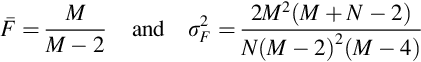
Note that the mean of the F-probability density function approaches ![]() as M → ∞. For small values of M and N, the F-probability density function is skewed towards low values of F. At large values of M and N, it is more symmetric around F = 1. In MatLab, the F-probability density function is computed as
as M → ∞. For small values of M and N, the F-probability density function is skewed towards low values of F. At large values of M and N, it is more symmetric around F = 1. In MatLab, the F-probability density function is computed as
(MatLab eda12_04)
where F is a vector of F values.
12.4 A hypothesis testing scenario
The general procedure for determining whether a result is significant is to first state a Null Hypothesis, and then identify and compute a statistic whose value will probably be small if the Null Hypothesis is true. If the value is large, then the Null Hypothesis is unlikely to be true and can be rejected. The probability density function of the statistic is used to assess just how unlikely, given any particular value. Four Null Hypotheses are common:
(1) Null Hypothesis: The mean of a random variable differs from a prescribed value only because of random fluctuation. This hypothesis is tested with the statistic, Z or t, depending on whether the variance of the data is known beforehand or estimated from the data. The tests of significance use the Z-probability density function or t-probability density function, and are called the Z-test and the t-test, respectively.
(2) Null Hypothesis: The variance of a random variable differs from a prescribed value only because of random fluctuation. This hypothesis is tested with the statistic, χN2, and the corresponding test is called the chi-squared test.
(3) Null Hypothesis: The means of two random variables differ from each other only because of random fluctuation. The Z-test or t-test is used, depending on whether the variances are known beforehand or computed from the data.
(4) Null Hypothesis: The variances of two random variables differ from each other only because of random fluctuation. The F-test is used.
As an example of the use of these tests, consider the following scenario. Suppose that you are conducting research that requires measuring the sizes of particles (e.g., aerosols) in the 10-1000 nm range. You purchase a laboratory instrument capable of measuring particle diameters. Its manufacturer states that (1) the device is extremely well-calibrated, in the sense that particles diameters will exactly scatter about their true means, and (2) that the variance of any single measurement is σd2 = 1 nm2. You test the machine by measuring the diameter, di, of N = 25 specially purchased calibration particles, each exactly 100 nm in diameter. You then use these data to calculate a variety of useful statistics (Table 12.1) that you hope will give you a sense about how well the instrument performs. A few weeks later, you repeat the test, using another set of calibration particles.
Table 12.1
Statistics arising from two calibration tests.
| Calibration Test 1 | Calibration Test 2 | Inter-Test Comparison | ||
| 1 | N | 25 | 25 | |
| 2 | 100 | 100 | ||
| 3 | 100.055 | 99.951 | ||
| 4 | 1 | 1 | ||
| 5 | 0.876 | 0.974 | ||
| 6 | 0.910 | 1.012 | ||
| 7 |  | 0.278 | 0.243 | |
| 8 | 0.780 | 0.807 | ||
| 9 |  | 21.921 | 24.353 | |
| 10 | 0.640 | 0.499 | ||
| 11 |  | 0.297 | 0.247 | |
| 12 | 0.768 | 0.806 | ||
| 13 | 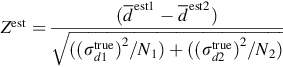 | 0.368 | ||
| 14 | 0.712 | |||
| 15 |  | 0.376 | ||
| 16 |  | 48 | ||
| 17 | 0.707 | |||
| 18 | 1.110 | |||
| 19 | 0.794 | |||

The synthetic data for these tests that we analyze below were drawn from a Normal probability density function with a mean of 100 nm and a variance of 1 nm2 (MatLab script eda12_05). Thus, the data do not violate the manufacturer's specifications and (hopefully) the statistical tests should corroborate this.
Question 1: Is the calibration correct? Because of measurement noise, the estimated mean diameter, ![]() , of the calibration particles will always depart slightly from the true value,
, of the calibration particles will always depart slightly from the true value, ![]() , even if the calibration of the instrument is perfect. Thus, the Null Hypothesis is that the observed deviation of the average particle size from its true value is due to observational error (as contrasted to a bias in the calibration). If the data are Normally distributed, so is their mean, with the variance being smaller by a factor of 1/√N. The quantity,
, even if the calibration of the instrument is perfect. Thus, the Null Hypothesis is that the observed deviation of the average particle size from its true value is due to observational error (as contrasted to a bias in the calibration). If the data are Normally distributed, so is their mean, with the variance being smaller by a factor of 1/√N. The quantity, ![]() (Table 12.1, row 7), which quantifies how different the observed mean is from the true mean, is Normally distributed with zero mean and unit variance. It has the value Z est = 0.278 for the first test and Z est = 0.243 for the second. The critical question is how frequently Zs of this size or larger occur. Only if they occur extremely infrequently can the Null Hypothesis be rejected. Note that a small Z is one that is close to zero, regardless of its sign, so the absolute value of Z is the quantity that is tested—a two-sided test. The Null Hypothesis can be rejected only when values greater than or equal to the observed Z are very uncommon; that is, when P(|Z| ≥ Z est) is small, say less than 0.05 (or 5%). We find (Table 12.1, row 8) that P(|Z| ≥ Z est) = 0.78 for test 1 and 0.81 for test 2, so the Null Hypothesis cannot be rejected in either case.
(Table 12.1, row 7), which quantifies how different the observed mean is from the true mean, is Normally distributed with zero mean and unit variance. It has the value Z est = 0.278 for the first test and Z est = 0.243 for the second. The critical question is how frequently Zs of this size or larger occur. Only if they occur extremely infrequently can the Null Hypothesis be rejected. Note that a small Z is one that is close to zero, regardless of its sign, so the absolute value of Z is the quantity that is tested—a two-sided test. The Null Hypothesis can be rejected only when values greater than or equal to the observed Z are very uncommon; that is, when P(|Z| ≥ Z est) is small, say less than 0.05 (or 5%). We find (Table 12.1, row 8) that P(|Z| ≥ Z est) = 0.78 for test 1 and 0.81 for test 2, so the Null Hypothesis cannot be rejected in either case.
MatLab provides a function, normcdf(), that computes the cumulative probability of the Normal probability density function:

The probability that Z is between −Z est and +Z est is P(|Z est|) − P(−|Z est|). Thus, the probability that Z is outside this interval is P(|Z| ≥ Z est) = 1 − [P(|Z est|) − P(−|Z est|)]. In MatLab, this probability is computed as
PZA = 1 − (normcdf(ZA,0,1)−normcdf(−ZA,0,1));
(MatLab eda12_06)
where ZA is the absolute value of Z est. The function, normcdf(), computes the cumulative Z-probability distribution (i.e., the cumulative Normal probability distribution).
Question 2: Is the variance within specs? Because of measurement noise, the estimated variance, ![]() , of the diameters of the calibration particles will always depart slightly from the true value,
, of the diameters of the calibration particles will always depart slightly from the true value, ![]() , even if the instrument is functioning correctly. Thus, the Null Hypothesis is that the observed deviation is due to random fluctuation (as contrasted to the instrument really being noisier than specified). The quantity,
, even if the instrument is functioning correctly. Thus, the Null Hypothesis is that the observed deviation is due to random fluctuation (as contrasted to the instrument really being noisier than specified). The quantity, ![]() (Table 12.1, row 9) is chi-squared distributed with 25 degrees of freedom. It has a value of,
(Table 12.1, row 9) is chi-squared distributed with 25 degrees of freedom. It has a value of, ![]() for the first test and 24.4 for the second. The critical question is whether these values occur with high probability; if so, the Null Hypothesis cannot be rejected. In this case, we really care only if the variance is worse than what the manufacturer stated, so a one-sided test is appropriate. That is, we want to know the probability that a value is greater than
for the first test and 24.4 for the second. The critical question is whether these values occur with high probability; if so, the Null Hypothesis cannot be rejected. In this case, we really care only if the variance is worse than what the manufacturer stated, so a one-sided test is appropriate. That is, we want to know the probability that a value is greater than ![]() . We find that
. We find that ![]() for test 1 and 0.50 for test 2. Both of these numbers are much larger than 0.05, so the Null Hypothesis cannot be rejected in either case. In MatLab, the probability,
for test 1 and 0.50 for test 2. Both of these numbers are much larger than 0.05, so the Null Hypothesis cannot be rejected in either case. In MatLab, the probability, ![]() is calculated as follows:
is calculated as follows:
Pchi2A = 1 − chi2cdf(chi2A,NA);
(MatLab eda12_07)
Here, chi2A is ![]() and NA stands for the degrees of freedom (25, in this case). The function, chi2cdf(), computes the cumulative chi-squared probability distribution.
and NA stands for the degrees of freedom (25, in this case). The function, chi2cdf(), computes the cumulative chi-squared probability distribution.
Question 1, Revisited: Is the calibration correct? Suppose that the manufacturer had not stated a variance. We cannot form the quantity, Z, as it depends on the variance, ![]() , which is unknown. However, we can estimate the variance from the data,
, which is unknown. However, we can estimate the variance from the data, ![]() . But because this estimate is a random variable, we cannot use it in the formula for Z, for Z would not be Normally distributed. Such a quantity would instead be t-distributed, as can be seen from the following:
. But because this estimate is a random variable, we cannot use it in the formula for Z, for Z would not be Normally distributed. Such a quantity would instead be t-distributed, as can be seen from the following:

Note that we have inserted σdtrue/σdtrue into the denominator of the third term in order to normalize di and ![]() into random variables, ei and e, that have unit variance. In our case, t est = 0.294 for test 1 and 0.247 for test 2.
into random variables, ei and e, that have unit variance. In our case, t est = 0.294 for test 1 and 0.247 for test 2.
The Null Hypothesis is the same as before; that the observed deviation of the average particle size is due to observational error (as contrasted to a bias in the calibration). We again use a two-sided test and find that P(|t| ≥ t est) = 0.77 for test 1 and 0.81 for test 2. These probabilities are much higher than 0.05, so the Null Hypothesis cannot be rejected in either case. In MatLab we compute the probability as
PtA = 1 − (tcdf(tA,NA)−tcdf(−tA,NA));
(MatLab eda12_07)
Here, tA is |t est| and NA = 25 denotes the degrees of freedom (25 in this case). The function, tcdf(), computes the cumulative t-probability distribution.
Question 3: Has the calibration changed between the two tests? The Null Hypothesis is that any difference between the two means is due to random variation. The quantity, ![]() , is Normally distributed, as it is a linear function of two Normally distributed random variables. Its variance is just the sum of the variances of the two terms (see Table 12.1, row 13). We find Z est = 0.368 and P(|Z| ≥ Z est) = 0.712. Once again, the probability is much larger than 0.05, so the Null Hypothesis cannot be excluded.
, is Normally distributed, as it is a linear function of two Normally distributed random variables. Its variance is just the sum of the variances of the two terms (see Table 12.1, row 13). We find Z est = 0.368 and P(|Z| ≥ Z est) = 0.712. Once again, the probability is much larger than 0.05, so the Null Hypothesis cannot be excluded.
Question 3, Revisited. Note that in the true variances, (σd1true)2 and (σd2true)2 are needed to form the quantity, Z (Table 12.1, row 13). If they are unavailable, then one must estimate variances from the data, itself. This estimate can be made in either of two ways

depending on whether the true mean of the data is known. Both are random variables and so cannot be used to form Z, as it would not be Normally distributed. An estimated variance can be used to create the analogous quantity, t (Table 12.1, row 15), but such a quantity is only approximately t-distributed, because the difference between two t-distributed variables is not exactly t-distributed. The approximation is improved by defining effective degrees of freedom, M (as in Table 12.1, row 16). We find in this case that test = 0.376 and M = 48. The probability P(|t| ≥ test) = 0.71, which is much larger than the 0.05 needed to reject the Null Hypothesis.
Question 4. Did the variance change between tests? The estimated variance is 0.876 in the first test and 0.974 in the second. Is it possible that it is getting worse? The Null Hypothesis is that the difference between these estimates is due to random variation. The quantity, F (Table 12.1, row 18), is defined as the ratio of the sum of squares of the two sets of measurements, and is thus proportional to the ratio of their estimated variances. In this case, Fest = 1.11 (Table 12.1, row18). An F that is greater than unity implies that the variance appears to get larger (worse). An F less than unity would mean that the variance appeared to get smaller (better). As F is defined in terms of a ratio, 1/Fest is as better as Fest is worse. Thus, a two-sided test is needed to assess whether the variance is unchanged (neither better nor worse); that is, one based on the probability, P(F ≤ 1/Fest or F ≥ Fest), which in this case is 0.79. Once again, the Null Hypothesis cannot be rejected.
The MatLab code for computing P(F ≤ 1/Fest or F ≥ Fest) is
if(F<1)
 F=1/F;
end
PF = 1 − (fcdf(F,NA,NB)−fcdf(1/F,NA,NB));
(MatLab eda12_07)
The function, fcdf(), computes the cumulative F-probability distribution. Note that F is replaced with its reciprocal if it is less than unity. Here NA and NB are the degrees of freedom of tests 1 and 2, respectively (both 25, in this case).
We summarize below what we have learned about the instrument:
Question 1: Is the calibration correct? Answer: We cannot reject the Null Hypothesis that the difference between the estimated and manufacturer-stated calibration is caused by random variation.
Question 2: Is the variance within specs? Answer: We cannot reject the Null Hypothesis that the difference between the estimated and manufacturer-stated variance is caused by random variation.
Question 3: Has the calibration changed between the two tests? Answer: We cannot reject the Null Hypothesis that difference between the two calibrations is caused by random variation.
Question 4. Did the variance change between tests? Answer: We cannot reject the Null Hypothesis that difference between the two estimated variances is caused by random variation.
Note that in each case, the results are stated with respect to a particular Null Hypothesis.
12.5 Chi-squared test for generalized least squares
In the previous section, we developed a chi-squared test to assess the Null Hypothesis that an estimated (posterior) variance differs from a prescribed (prior) value only because of random variation. As discussed in Section 4..8, the posterior variance can be estimaed from the error of fit (Equation 4.31), such as the fit of a model determined by generalized least squares. Thus, we can use a chi-squared test to assess the following:
Null Hypothesis
The difference of the generalized error from its expected value is due to random variation.
The generalized error ET is the sum of two terms (Equation 5.15):
The first term is the estimated error Eobs in the data:

and the second term is the estimated error Epest in the prior information:

The data vector d has length N, the prior information vector h has length K and the model parameter vector m has lengtth M. The variance σd2 of the data and the variance σh2 of the prior information are prior variances; that is, they have been determined by a method unrelated to the least squares estimation process. For instance, σd2 could be based on the published precision of a laboratory apparatus (e.g. the manufacturer stated accuracy) and σd2 could be based on a typical range of variation of the particular kind of prior information, as published in the scientific literature (most measurements of this kind are within a known percent of a stated value).
The total error is the sum of squares of Normally-distributed random variables, each with unit variance, and so is chi-squared distributed. The number of degrees of freedom νT is the number ![]() of component errors reduced by the number M of model parameters, so
of component errors reduced by the number M of model parameters, so ![]() . The reduction reflects the notion that the data and prior information can be fit exactly when
. The reduction reflects the notion that the data and prior information can be fit exactly when ![]() , yielding a posterior variance of zero. The total error has mean νT and variance 2νT, and the 95% confidence interval is approximately:
, yielding a posterior variance of zero. The total error has mean νT and variance 2νT, and the 95% confidence interval is approximately:
The generalized least squares error is incompatible with the prior variances σd2 and σh2 only when it falls outside this interval; that is, the Null Hypothesis is unlikely in this case. Errors that are to the right of the interval correspond to models that fit the data more poorly than can be expected by random variation alone. A poor fit case can occur when the model is too simple. Too few model parameters are availble to capture the true variability of the data and prior information. Errors to the left of the interval correspond to models that overfit the data; that is, the error is smaller than can be expected by random variation alone. The overfit case can occur when the model is too complex. So many model parameters are available that even the noise is being fit.
The individual compatibility of the errors Eest and of Epest with their respective prior variances can also be tested. These errors are chi-squared distributed, but with fewer degres of error than the total error ETest. An important issue is how to partition the loss of degrees of freedom associated with the M model parameters between Eest and Epest. The Welch–Satterthwaite approximation spreads it in proportion to the number of component errors, so that Eest is assigned ![]() degrees of freedom and Epobs is assigned
degrees of freedom and Epobs is assigned ![]() degrees of freedom. The 95% confidence intervals are approximately:
degrees of freedom. The 95% confidence intervals are approximately:
Crib Sheet 12.1
Steps in generalized least squares
Step 1: State the problem in words
How are the data related to the model
Step 2: Organize the problem in standard form
identify the data d (length N) the model parameters m (length ![]()
define the data kernel G so that ![]()
make plots of the data
Step 4: Establish the accuracy of the data
state a prior variance σd2 based on accuracy of the measurement technique
Step 5: State the prior information in words, for example:
the model parameters are close to a known values, hpri
the mean of the model parameters is close to a known value
the model parameters vary smoothly with space and time
Step 6: Organize the prior information in standard form:
Step 7: Establish the accuracy of the prior information
state a prior variance σh2 based on the accuracy of the prior information
Step 8: Estimate model parameter mest and their covariance Cm

Step 9: State estimates and their 95% confidence intervals
Step 10: Examine the individual errors
plot ei vs. i and plot epi vs. i
scatter plot of dipre vs. diobs and scatter plot of hipre vs. hipri
any unusually large errors?
Step 11: Examine the total error ET
use a chi-squared test on ET to assess the likelihood of the Null Hypothesis that ET is different than expected only because of random variation
Step 12: Two different models?
use an F-test on the E’s of the two models to assess the likelihood
of the Null Hypothesis that the E’s are
different from each other only because of random variation
12.6 Testing improvement in fit
Very common is the situation where two alternative models are proposed for a single dataset. Neither fits the data exactly, but one has a smaller total error, E, than the other. Calling the model with the smaller corresponding error the better-fitting model is natural. Recall, however, that the error, E, is a random variable. Different realizations of it will vary in size, even when drawn from probability density functions with the exactly the same mean. Thus, when the two errors are similar in size, their difference may be due to random variation and not to one model “really” being better than the other.
The F-test is used to assess the significance in the ratio of the estimated variance of the two fits (Figure 12.4):


Here, the first model has M1 model parameters, N1 data, and a total error, E1 and the second model has M2 model parameters, N2 data, and a total error, E2. Note that a model with M parameters ought to be able to fit a dataset with N = M data exactly, so the degrees of freedom are K = N − M. If the variances of individual errors, ei, used to compute the Es are all equal, then they cancel out of the fraction, E1/E2. Thus, the statistic, F, does not depend on the variance of the data and one is free to use the unweighted error, E = Σi (diobs − dipre)2.
As an example, we consider the rising temperatures during the first 60 h of the Black Rock Forest dataset (Figure 12.5). A straight line (Figure 12.5A) fits the data fairly well, but a cubic function fits it better, with F = 1.112. The Null Hypothesis is that both functions fit the data equally well, and that the difference in error is due to random variation. A two-sided test gives

P(F ≤ 1/Fest or F ≥ Fest) = 0.71, which is much larger than 0.05, so the Null Hypothesis that the fits are equally good cannot be rejected.
12.7 Testing the significance of a spectral peak
A complicated time series, meaning one with many short-period fluctuations, usually has a complicated spectrum, with many peaks and troughs. Some peaks may be particularly high-amplitude and stand above other lower-amplitude ones. We would like to know whether the high-amplitude peaks are significant. Pinning down just what we mean by significant requires some careful thinking.
Suppose that the data consists of a cosine wave of amplitude, A, with just a little random observational noise superimposed on it. We could employ the rules of error propagation to compute how the variance, σd2, of the observations leads to variance, σA2, in our estimate of the amplitude, A, and then state the confidence intervals for the amplitude as A ± 2σA. We could then test whether a peak has an amplitude significantly different from a prescribed value, or test whether two peaks have amplitudes that are significantly different from each other, or so forth.
The problem is that this is almost never what we mean by the significance of a spectral peak. The much more common scenario is one in which a long and possibly continuous time series is dominated by “noise” that has no obvious sinusoidal patterns at all. Furthermore, the noise is usually some complicated and unmodeled part of the time series itself, and not observational error in the strict sense. We take the spectrum of a portion of the time series—the first hour, say—and detect a spectral peak at frequency, f0. We want to know if this peak is significant in the sense that, if we were to take the spectra of subsequent hourly segments, they would also have peaks at frequency, f0. The alternative is that the observed peak arises from some “accident” of the noise pattern in that particular hour of data that is not shared by the other hourly segments.
The Null Hypothesis that corresponds to this case is that the spectral peak can be explained by random variation within a time series that consists of nothing but random noise. The easiest case to analyze is a time series that consists of nothing but uncorrelated, Normally distributed random noise with constant variance. The power spectral density of such a time series will have peaks, and the height of these peaks has a probability density function that will allow us to quantify the likelihood that the height of a peak will exceed a specified value. If the likelihood of an observed peak is low, then we have reason to reject the Null Hypothesis and claim that the peak is significant, in the sense of being unlikely to have arisen from random fluctuations.
Before starting the analysis, we need to carefully specify whether Fourier coefficients are defined in the frequency range, (0, fny) or (−fny, fny), because the former have twice the amplitude of the latter. We choose the former, for then plotting power spectral density on the (0, fny) interval, which is the shorter of the two, seems more natural.
Suppose that time series, di, of length, N, consists of uncorrelated random noise with zero mean and variance, σd2. Before computing the Fourier transform, the time series is modified by multiplication with a taper, wi, so that it has elements, widi. The variance of the tapered time series is N−1Σi=1Nwi2di2, but this is approximately ffσd2, where ff = N−1Σi=1Nwi2 is the variance of the taper. This can be seen from the N = 3 example:

The approximation holds because all the ds have the same statistical properties, so their order has little influence on the sums. This behavior suggests that we normalize the taper to unit variance, ff = 1, so that it has the least effect on the variance of the data (and hence on the overall power in the power spectral density). However, in the discussion, below, we allow ff to have an arbitrary value.
When the data are uncorrelated and Normally distributed, with uniform variance and zero mean, the coefficients of their Fourier series are also uncorrelated and Normally distributed, with uniform variance and zero mean. This follows from the fact that the Fourier transform is a linear function of the data of the form, Gm = d, where m is a vector of the Fourier coefficients, together with the relationship, [GTG]−1 ∝ I (Equation 6.14) (except for the first and last frequencies, which we will ignore in this analysis). Each element of the power spectral density, s2(t), is proportional to the sum of squares of two Fourier coefficients. If we normalize the Fourier coefficients to unit variance, then the power spectral density is chi-squared distributed with p = 2 degrees of freedom. The normalization factor, c, is calculated using the relationship between the variance of the time series and the frequency integral of the power spectral density (Equation 6.44), together with the fact that a chi-squared probability density function with two degrees of freedom has mean, 2, and variance, 4:

Here, Nf = N/2 + 1. Hence, the power spectral density has mean, ![]() given by
given by
Thus, we need know only the basic parameters that define a random time series—the ones that make up the constant, c—in order to predict the statistical properties of its power spectral density (Figures 12.6 and 12.7). The probability that an element of the power spectral density will exceed a given value, say ![]() , is 1 − P(
, is 1 − P(![]() /c), where P is the cumulative chi-squared distribution with two degrees of freedom.
/c), where P is the cumulative chi-squared distribution with two degrees of freedom.


As an example, we consider a length N = 1024 time series built up from a 5 Hz cosine wave plus uncorrelated noise, drawn from a Normal probability density function with zero mean and variance, σd2. The amplitude of the cosine is chosen to be small, only 0.25σd, so that its presence cannot be detected readily though visual inspection of the time series (Figure 12.8A). Nevertheless, the power spectral density (Figure 12.8B) has a prominent peak at 5 Hz, with height, ![]() , approximately 10 times the mean level (Figure 12.9). The probability that an element of the power spectral density will have a probability at or below this level can be calculated using MatLab's inverse chi-squared probability distribution:
, approximately 10 times the mean level (Figure 12.9). The probability that an element of the power spectral density will have a probability at or below this level can be calculated using MatLab's inverse chi-squared probability distribution:


(MatLab eda12_11)
Here, speak is s02, c is the constant defined in Equation 12.23, and p=2 denotes the degrees of freedom. We find that ppeak=0.99994, which is to say that the power spectral density is predicted to be less than the level, s02, 99.994% of the time.
At this point, we must be exceedingly careful in stating the Null Hypothesis. If we are specifically looking for a 5-Hz oscillation, then the Null Hypothesis would be that a peak at 5-Hz arose solely by random variation. In this case, the probability is 1 − 0.99994 = 0.00006 or 0.006%, which is very small, indeed. Thus, we can reject the Null Hypothesis with very high confidence. However, this analysis relies on prior knowledge that 5 Hz is special—that a peak occurs there.
Instances will indeed arise when we suspect spectral peaks at specific frequencies—the annual and diurnal periodicities that we discussed in the context of the Black Rock Forest temperature dataset are examples. But another common scenario is one where we have no special knowledge about what frequencies might be associated with peaks. We see a peak somewhere in the power spectral density and want to know whether or not it is significant. In this case, the Null Hypothesis is that any peak at any frequency in the record arose solely by random variation.
In this example, the power spectral density has N/2 + 1 = 513 elements. Thus, there are 513 independent chances for a peak to occur. The probability that a peak of amplitude, ![]() , occurs somewhere among those 513 possibilities is (0.99994)513 = 0.97. Thus, there is a 3% chance that a peak arose from random variation—still a small probability, but much larger than the 0.006% that we calculated previously We can still reject the Null Hypothesis at greater than 95% confidence, but with much less confidence than before.
, occurs somewhere among those 513 possibilities is (0.99994)513 = 0.97. Thus, there is a 3% chance that a peak arose from random variation—still a small probability, but much larger than the 0.006% that we calculated previously We can still reject the Null Hypothesis at greater than 95% confidence, but with much less confidence than before.
Crib Sheet 12.2
Computing power spectral density
Step 1, Compute time and frequency parameters
number N of data should be even (truncate if necessary)
duration of time series, T=N*Dt;
Nyquist (maximum) frequency, fmax=1/(2*Dt);
frequency interval, Df = fmax/(N/2);
number of non-negative frequencies, Nf=N/2+1;
frequency vector, f=Df*[0:N/2,-N/2+1:-1]';
Step 2: Pre-process time series, d(t)
subtract mean, d = d-mean(d);
apply Hamming window function,
w=0.54-0.46*cos(2*pi*[0:N-1]'’/(N-1));
dw=w.*d;
Step 3: Compute Fourier Transform, ![]()
dtilde = Dt * fft(dw);
dtilde = dtilde[1:Nf];
Step 4: Compute power spectral density, s2(f)
s2=(2/T)*abs(dtilde).ˆ2;
Step 5: Plot power spectral density and look for peaks
plot( f(1:Nf), s2, ‘k-’ );
Step 6: Compute 95% confidence level
Null Hypothesis: time series is uncorrelated random noise
variance of time series, s2est=std(d);
power in window function, ff=sum(w.*w)/N;
scaling constant, c = (ff*sd2est)/(2*Nf*Df);
95% confidence level, cl95 = c*chi2inv(0.95,2);
Step 7: Plot confidence level and assess significance of peaks
plot([f(1), f(Nf)], [cl95, cl95], 'k-');
12.8 Bootstrap confidence intervals
Many special-purpose statistical tests have been put forward in the literature. Each proposes a statistic appropriate for a specific data analysis scenario and provides a means for testing its significance. However, data analysis scenarios are extremely varied and many have no well-understood tests. Sometimes, model parameters will have a sufficiently complicated relationship to the data that error propagation by normal means will be impractical, making the determination of confidence intervals difficult.
Consider a scenario in which a model parameter, m, is determined through a complicated data analysis procedure. If a large number of repeated datasets are available—repeated in the sense of having made all the measurements again at another time—then the problem of determining confidence intervals for the parameter, m, could be approached empirically. The same analysis could be performed on each dataset and a histogram for parameter, m, constructed. With enough repeat datasets, the histogram will approximate the probability density function, p(m). Confidence intervals could then be derived from p(m). While true repeat datasets are seldom available, this method will also work if approximate repeat datasets could somehow be constructed from the single, available dataset.
A dataset, d, can be viewed as consisting of N realizations of the probability density function, p(d). The probability density function, p(d), itself can be viewed—loosely—as containing an infinite number of realizations. Suppose that we construct another probability density function, p′(d), by duplicating the N realizations an indefinite number of times and mixing them together (Figure 12.10). As N → ∞, p′(d) → p(d). As long as N is large enough, p′(d) will be an adequate approximation to p(d).

This scenario suggests that an approximate repeat dataset can be created by randomly resampling the original dataset with duplications. If the original data are in a column-vector, dorig, then a new dataset, d, is constructed by randomly choosing an element from dorig each of N times. The two datasets will not be the same, because duplicates from dorig are allowed in d. Furthermore, many such resampled datasets can be constructed, all distinct from one another. Identical analyses can then be performed on each resampled dataset, and a histogram of the estimated model parameters assembled. This procedure is called the bootstrap method.
We start with a simple case—determining confidence intervals for the slope, b, of a straight line fit to data. We already know how to determine confidence intervals for this linear problem, so it provides a good way to verify the bootstrap results. The probability density function, p(b), of the slope is Normal with variance, σ2b, given by a simple formula (Equation 4.29), so 95% confidence is within ±2σb of the mean.
The bootstrap method contains two steps, both within a loop over the number, Nr, of times that the original data are resampled. In the first step, the data, dorig, and corresponding times, torig, are resampled into d and t. In the second step, standard methodology (least-squares, in this case) is used to estimate the parameter of interest (slope, b, in this case) from d and t.
for p = [1:Nr]
 % resample
 rowindex=unidrnd(N,N,1);
 t = torig(rowindex);
 d = dorig(rowindex);
 % straight line fit
 M=2;
 G=zeros(N,M);
 G(:,1)=1;
 G(:,2)=t;
 mest=(G'*G)(G'*d);
 slope(p)=mest(2);
end
(MatLab eda12_12)
The rowindex array specifies how the original data are resampled. It is created with the unidrnd() function, which returns a column-vector of random integers between 1 and N. The end result is a length-Nr column-vector of slopes. A histogram can then be formed from these slopes and converted into an estimate of the probability density, p(b):
Nbins = 100;
[shist, bins]=hist(slope, Nbins);
Db = bins(2)−bins(1);
pbootstrap = shist / (Db*sum(shist));
(MatLab eda12_12)
The last line turns the histogram into a properly normalized probability density function, pbootstrap, with unit area (Figure 12.11). As expected in this case, the probability density function, p(b), is a good approximation to the Normal probability density function predicted by the standard error propagation formulas. We can use this probability density function to derive estimates of the mean and variance of the slope (see Equations 3.3 and 3.4):

mb = Db*sum(bins.*pbootstrap);
vb = Db*sum(((bins−mb).○2).*pbootstrap);
(MatLab eda12_12)
Here, mb is the mean and vb is the variance of the slope, b. As the probability density function is approximately Normal, we can state the 95% confidence interval as mb±2√vb. However, in other cases, the probability density function may be nonNormal, in which case an explicit calculation of confidence is more accurate:
Pbootstrap = Db*cumsum(pbootstrap);
ilo = find(Pbootstrap >= 0.025,1);
ihi = find(Pbootstrap >= 0.975,1);
blo = bins(ilo);
bhi = bins(ihi);
(MatLab eda12_12)
Here, the cumsum() function is used to integrate the probability density function into a probability distribution, Pbootstrap, and the find() function is used to find the values of slope, b, that enclose 95% of the total probability. The 95% confidence interval is then, blo < b < bhi.
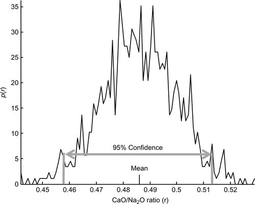
In a more realistic example, we return to the varimax factor analysis that we performed on the Atlantic Rock dataset (Figure 8.6). Suppose that the CaO to Na2O ratio, r, of factor 2 is of importance to the conclusions drawn from the analysis. The relationship between the data and r is very complex, involving both singular-value decomposition and varimax rotation, so deriving confidence intervals by standard means is impractical. In contrast, bootstrap estimation of p(r), and hence the confidence intervals of r, is completely straightforward (Figure 12.12).
Problems
12.1 The first and twelfth year of the Black Rock Forest temperature dataset are more-or-less complete. After removing hot and cold spikes, calculate the mean of the 10 hottest days of each of these years. Test whether the means are significantly different from one another by following these steps: (A) State the Null Hypothesis. (B) Calculate the t-statistic for this case. (C) Can the Null Hypothesis be rejected?
12.2 Revisit Neuse River prediction error filters that you calculated in Problem 7.2 and analyze the significance of the error reduction for pairs of filters of different length.
12.3 Formally show that the quantity, ![]() , has zero mean and unit variance, assuming that d is Normally distributed with mean,
, has zero mean and unit variance, assuming that d is Normally distributed with mean, ![]() , and variance, σd2, by transforming the probability density function, p(d) to p(Z).
, and variance, σd2, by transforming the probability density function, p(d) to p(Z).
12.4 Figure 12.6B shows the power spectral density of a random time series. A) Count up the number of peaks that are significant to the 95% level or greater and compare with the expected number. B) What is the significance level of the highest peak? (Note that N = 1024 and c = 0.634 for this dataset).
12.5 Analyze the significance of the major peaks in the power spectral density of the Neuse River Hydrograph (see Figure 6.11 and MatLab script eda06_13).