6.1 Describing sinusoidal oscillations

Sinusoidal oscillations—those involving sines and cosines—are very common in the environmental sciences. We encountered them in the Neuse River Hydrograph and the Black Rock Forest datasets, where they were associated with seasonal variations in river discharge and air temperature, respectively. This chapter examines oscillatory behavior in more detail, developing systematic methods for detecting and quantifying periodicities.

Periodicities can be both temporal and spatial in character, with a somewhat different nomenclature used for each. In both cases, the height of the oscillation is called its amplitude. Temporal periodicities have a period, T, the time between successive cycles. Spatial periodicities have a wavelength, λ, the distance between successive cycles. The rate at which temporal cycles occur is called the frequency and the rate at which spatial cycles occur is called wavenumber. Frequency can be measured in units of cycles per unit time, in which case it is given the symbol, f, or it can be measured in units of radians per unit time, in which case it is given the symbol, ω. The units of cycles per second are called Hertz, abbreviated Hz. Similarly, wavenumber can be measured in either cycles per unit distance or radians per unit distance. Unfortunately, both units of wavenumber tend to be given the same symbol, k, in the literature. In this book, we use k exclusively to mean radians per unit distance. These quantities are related as follows:

$f=\frac{1}{T}=\frac{\omega }{2\pi }\text{and}\frac{1}{\lambda }=\frac{k}{2\pi }$

Generic temporal, d(t), and spatial, d(x), cosine oscillations of amplitude, C, can be written as

$d(t)=Ccos\left\{\frac{2\pi t}{T}\right\}=Ccos\{2\pi ft\}=Ccos\{\omega t\}\text{and}d(x)=Ccos\left\{\frac{2\pi x}{\lambda }\right\}=Ccos\{kx\}$

In nature, oscillations rarely “start” at time (or distance) zero. A cosine wave with amplitude, C, that starts (peaks) at time, t₀, is given by (Figure 6.1)

$d(t)=Ccos\left\{\frac{2\pi (t-t_0)}{T}\right\}=Ccos\{\omega (t-t_0)\}=Ccos\{\omega t-\varphi \}$

The quantity, ϕ = ωt₀, is called the phase. The rule,

$\mathit{cos}(a-b)=\mathit{cos}(a)\mathit{cos}(b)+\mathit{sin}(a)\mathit{sin}(b)$

when applied to Equation (6.3), yields

$\begin{array}{l}d(t)=Ccos\{\omega (t-t_0)\}\hfill \\ =Ccos(\omega t_0)cos(\omega t)+Csin(\omega t_0)sin(\omega t)=\text{A}cos(\omega t)+\text{B}sin(\omega t)\hfill \\ \text{with}\hfill \\ A=C\text{cos}(\omega t_0)\text{and}B=C\text{cos}(\omega t_0)\hfill \\ \text{and}\hfill \\ C=\sqrt{A^2+B^2}\text{and}{t}_0={\omega }^{-1}{tan}^{-1}(B/A)\hfill \end{array}$

See Note 6.1 for a discussion of how the arc-tangent is to be correctly computed. A time-shifted cosine can be represented as the sum of a sine and a cosine. An explicit time-shift variable such as t₀ is unnecessary in formulas describing periodicities, as long as sines and cosines are paired up with one another.

6.2 Models composed only of sinusoidal functions

Suppose that we have a dataset in which a variable, such as temperature, is sampled at evenly spaced intervals of time, t_i (a time series), say with sampling interval, Δt. One extreme is a dataset composed of only sinusoidal oscillations:

$\begin{array}{ll}\text{the data}& =\text{sum of sines and cosines}\\ d(t_i)& ={\text{A}}_{1}cos({\omega }_1{t}_i)+{\text{B}}_{1}sin({\omega }_1{t}_i)+{\text{A}}_{2}cos({\omega }_{2}t)+{\text{B}}_{2}sin({\omega }_{2}t)+\dots \end{array}$

This formula is sometimes referred to as a Fourier series or an inverse discrete Fourier transform and the column vector containing the As and Bs is called the discrete Fourier transform (DFT) of d. The As and Bs are the model parameters and the corresponding frequencies are taken to be auxiliary variables. Note that sines and cosines of a given frequency, ω_i, are paired, as was discussed in the previous section. Two key questions involve the number of frequencies that ought to be included in this representation and what their values should be. The answers to these questions involve a surprising fact about time series:

$\text{frequencies higher than}{f}_{\mathit{ny}}=\frac{1}{2\Delta t}\text{cannot be detected}$

This is called Nyquist's Sampling Theorem. It says that the periods shorter than two time increments cannot be detected in time series with evenly spaced samples. Furthermore, as we will see below, any frequencies in the data that are higher than the Nyquist frequency, f_ny, are erroneously mapped into the (0, f_ny) frequency range. Choosing the frequency range (0, f_ny) in Equation (6.5) is, therefore, natural. For simplicity, we assume that the number N of data is an even integer. It can always be made so by shortening an odd-length time series by one point. Then the number of frequencies is $N/2+1$ and the number M of unknown coefficients of cosines and sines exactly equals the number N of data; that is $M=N$. These choices imply

$f_{\mathit{ny}}=\frac{1}{2\Delta t}\text{and}{\omega }_{\mathit{ny}}=\frac{\pi }{\Delta t}\text{and}\Delta \omega =\frac{2\pi }{N\Delta t}\text{and}\Delta f=\frac{1}{N\Delta t}$

The reason that this relationship calls for ½N + 1, as contrasted to ½N of them, is that the first and last sine term is identically zero; that is,

$B_1\mathit{sin}(0t_i)=0\text{and}{B}_{(N/2)+1}\mathit{sin}\left(\frac{2\pi }{2\Delta t}{t}_i\right)=B_{(N/2)+1}\mathit{sin}(n\pi )=0$

where, n = t_i/Δt, is an integer. Hence, these two terms are omitted from the sum. Thus, the Fourier series contains the frequencies [0, Δf, 2Δf, …, ½NΔf]^T. The lowest frequency is zero. It corresponds to a cosine of zero period, that is, to a constant. The next highest frequency is Δf. It corresponds to a sine and a cosine that have one complete oscillation over the length of the data. The next highest frequency is 2Δf. It corresponds to a sine and a cosine that have two complete oscillations over the length of the data. The highest frequency is f_ny = ½NΔf = 1/(2Δt). It corresponds to a highly oscillatory cosine that reverses sign at every sample; that is [1, −1, 1, −1, …]^T (Figure 6.2).

In MatLab, frequency-related quantities are defined as follows:

Nf=N/2+1;
fmax = 1/(2*Dt);
Df = fmax/(N/2);
f = Df*[0:Nf−1]′;
Nw=Nf;
wmax = 2*pi*fmax;
Dw = wmax/(N/2);
w = Dw*[0:Nw−1]′

(MatLab script eda06_02)

Here, Dt is the sampling interval and N is the length of the data. N is assumed to be an even integer.

The problem that arises with frequencies higher than the Nyquist frequency can be seen by examining a pair of cosines and sines from Equation (6.6), written out for a particular time, t_k, and frequency, ω_n.

$\begin{array}{l}cos({\omega }_n{t}_k)=cos((n-1)(k-1)\Delta \omega \Delta t)=cos\left(\frac{2\pi (n-1)(k-1)}{N}\right)\hfill \\ sin({\omega }_n{t}_k)=sin((n-1)(k-1)\Delta \omega \Delta t)=sin\left(\frac{2\pi (n-1)(k-1)}{N}\right)\hfill \end{array}$

Here, we have used the rule, ΔωΔt = 2π/N. Note that we index time and frequency so that t₁ and ω₁ correspond to zero time and frequency, respectively; that is, t_k = (k−1)Δt and ω_n = (n−1)Δω. Now let us examine a frequency, ω_m, that is higher than the Nyquist frequency, say m = n + N, where N is the number of data:

$\begin{array}{ll}cos({\omega }_m{t}_k)\hfill & =cos((n-1+N)(k-1)\Delta \omega \Delta t)=cos\left(\frac{2\pi (n-1+N)(k-1)}{N}\right)\hfill \\ \hfill & =cos\left(\frac{2\pi (n-1)(k-1)}{N}\right)cos(2\pi (k-1))-sin\left(\frac{2\pi (n-1)(k-1)}{N}\right)sin(2\pi (k-1))\hfill \\ \hfill & =cos\left(\frac{2\pi (n-1)(k-1)}{N}\right)+0\hfill \\ sin({\omega }_m{t}_k)\hfill & =sin((n-1+N)(k-1)\Delta \omega \Delta t)=sin\left(\frac{2\pi (n-1+N)(k-1)}{N}\right)\hfill \\ \hfill & =sin\left(\frac{2\pi (n-1)(k-1)}{N}\right)cos(\pi (k-1))+cos\left(\frac{2\pi (n-1)(k-1)}{N}\right)sin(\pi (k-1))\hfill \\ \hfill & =sin\left(\frac{2\pi (n-1)(k-1)}{N}\right)+0\hfill \end{array}$

Here, we have used the rules, cos(a + b) = cos(a)cos(b) − sin(a)sin(b) and sin(a + b) = sin(a)cos(b) + cos(b)sin(a), together with the rule that cos(2π(k + 1)) = 1 and sin(2π(k + 1)) = 0, for any integer, k. Comparing Equations (6.10) and (6.11), we conclude

$cos({\omega }_n{t}_k)=cos({\omega }_m{t}_k)\text{and}sin({\omega }_n{t}_k)=sin({\omega }_m{t}_k)$

The frequencies, ω_n+N and ω_n, are equivalent, in the sense that they yield exactly the same sinusoids (Figure 6.3). A similar calculation, omitted here, shows that ω_N−n and −ω_n are equivalent in this same sense. But sines and cosines with negative frequencies have the same shape, up to a sign, as those with corresponding positive frequencies; that is, cos(−ωt) = cos(ωt) and sin(−ωt) = −sin(ωt). Thus, only sinusoids in the frequencies in the range ω₁ (zero frequency) to ω_N/2+1 (the Nyquist frequency) have unique shapes (Figure 6.3C). In a digital world, no frequencies are higher than the Nyquist.

This limitation implies that special care must be taken when observing a time series to avoid recording any frequencies that are higher than the Nyquist frequency. This goal is usually achieved by creating a data recording system that attenuates—or eliminates—high frequencies before the data are converted into digital samples. If any high frequencies persist, then the dataset is said to be aliased, and spurious low frequencies will appear.

The linear equation, d = Gm, form of the Fourier series is as follows:

$\begin{array}{c}\text{the data}=\text{sum of sines and cosines}\\ \left[\begin{array}{c}{d}_1\\ d_2\\ d_3\\ ⋮\\ d_N\end{array}\right]=\left[\begin{array}{ccccccc}1& \text{cos}({\omega }_2{t}_1)& \text{sin}({\omega }_2{t}_1)& \mathrm{\dots }& \text{cos}({\omega }_{N/2}{t}_1)& \text{sin}({\omega }_{N/2}{t}_1)& 1\\ 1& \text{cos}({\omega }_2{t}_2)& \text{sin}({\omega }_2{t}_2)& \mathrm{\dots }& \text{cos}({\omega }_{N/2}{t}_2)& \text{sin}({\omega }_{N/2}{t}_2)& -1\\ 1& \text{cos}({\omega }_2{t}_3)& \text{sin}({\omega }_2{t}_3)& \mathrm{\dots }& \text{cos}({\omega }_{N/2}{t}_3)& \text{sin}({\omega }_{N/2}{t}_3)& 1\\ 1& ⋮& ⋮& ⋮& ⋮& ⋮& ⋮\\ 1& \text{cos}({\omega }_2{t}_N)& \text{sin}({\omega }_2{t}_N)& \mathrm{\dots }& \text{cos}({\omega }_{N/2}{t}_N)& \text{sin}({\omega }_{N/2}{t}_N)& -1\end{array}\right]\left[\begin{array}{c}{A}_1\\ A_2\\ B_2\\ ⋮\\ A_{N/2}\\ B_{N/2}\\ A_{(N/2)+1}\end{array}\right]\end{array}$

In MatLab, the data kernel, G, is created as follows:

% set up G
G=zeros(N,M);
% zero frequency column
G(:,1)=1;
% interior M/2−1 columns
for i = [1:M/2−1]
 j = 2*i;
 k = j+1;
 G(:,j)=cos(w(i+1).*t);
 G(:,k)=sin(w(i+1).*t);
end
% nyquist column
G(:,M)=cos(w(Nw).*t);

(MatLab eda06_02)

Here, the number of model parameters, M, equals the number of data, N, and the frequency values are in a column vector, w.

Remarkably, the matrices, [G^TG] and [G^TG]⁻¹, which play such an important role in the least-squares solution, can be shown to be diagonal:

$\begin{array}{c}[{\mathbf{G}}^{\text{T}}\mathbf{G}]=N\text{diag}(1,½,½,\mathrm{\dots },½,½,1)\\ \text{and}\\ {[{\mathbf{G}}^{\text{T}}\mathbf{G}]}^{-1}=\frac{1}{N}\text{diag}(1,2,2,\mathrm{\dots },2,2,1)\end{array}$

Note that we have used the rule that the inverse of a diagonal matrix, M, is the matrix of reciprocals of the elements of the main diagonal; that is [M⁻¹]_ii = 1/M_ii. Equation (6.14) can be understood by noting that the elements of G^TG are just the dot products of the columns, c, of the matrix, G. Many of these dot products are clearly zero (meaning that [G^TG]_ij = c^(i)Tc^(j) = 0 when i ≠ j). For instance, the second column, cos(Δωt), is symmetric about its midpoint, while the third column, sin(Δωt), is antisymmetric about it, so their dot product is necessarily zero (see Figure 6.2B and C). What is not so clear—but nevertheless true—is that every column is orthogonal to every other. We will not derive this result here, for it requires rather nitty-gritty trigonometric manipulations (but see Note 6.2). Its consequence is that the least-squares solution, m = [G^TG]⁻¹G^Td requires only matrix multiplication, and not matrix inversion. Furthermore, when the data are uncorrelated, then the model parameters, m, which represent the amplitudes of the sines and cosines, are also uncorrelated, as C_m = σ²_d[G^TG]⁻¹ is diagonal. Furthermore, all but the first and last model parameters have equal variance.

In MatLab, the least-squares solution is computed as follows:

gtgi = 2* ones(M,1)/N;
gtgi(1)=1/N;
gtgi(M)=1/N;
mest=gtgi .* (G'*d);

(MatLab eda06_04)

The column vectors,

$\begin{array}{c}{[A_1^2,A_2^2+B_2^2,\dots ,A_{N/2}^2+B_{N/2}^2,A_{N/2+1}^2]}^{\text{T}}\\ \text{and}\\ {\left[\sqrt{A_1^2},\sqrt{A_2^2+B_2^2},\dots ,\sqrt{A_{N/2}^2+B_{N/2}^2},\sqrt{A_{N/2+1}^2}\right]}^{\text{T}}\end{array}$

are called the power spectral density and amplitude spectral density of the time series, respectively. Either can be used to quantify the overall amount of oscillations at any given frequency, irrespective of the phase. In MatLab, the power spectral density, s, is computed from mest as follows:

% zero frequency
s=zeros(Nw,1);
s(:,1)=mest(1)^2;
% interior points
for i = [1:M/2−1]
 j = 2*i;
 k = j+1;
 s(i+1) = mest(j)○2 + mest(k)^2;
end
% Nyquist frequency
s(Nw) = mest(M)^2;

(MatLab eda06_04)

When applied to the Neuse River discharge data, this method produces an amplitude spectral density that is largest at low frequencies (Figure 6.4A). In such cases, a graph with a logarithmic frequency axis (Figure 6.4B) allows one to see details that are squeezed near the origin of a linear plot (Figure 6.4A). In some applications, plotting amplitude spectral density as a function of period, as contrasted to frequency, may be preferable (as in this case, where the annual period of 365.2 days is more recognizable than the equivalent frequency of 0.002738 cycles/day). The amplitude spectral density consists of several peaks, superimposed on a “noisy background” that gradually declines with period. The three largest peaks have periods of 365.2, 182.6, and 60.2, (one, one-half, and one-sixth years) and are associated with oscillations in stream flow caused by seasonal fluctuations in rainfall.

A common practice is to omit the zero-frequency element of the spectral density from the plots (as was done here). It only reflects the mean value of the time series and is not really relevant to the issue of periodicities. Large values can require a vertical scaling that obscures the rest of the plot.

The MatLab script, eda06_04, worked fine calculating the spectral density of an N ≈ 4000 length time series. However, the N × N matrix, G, will become prohibitively large for larger datasets. Fortunately, a very efficient algorithm, called the fast Fourier transform (FFT), has been discovered for solving for m^est that requires much less storage and much less computation than “brute force” multiplication by G^T. We will return to this issue later in the chapter.

6.3 Going complex

Many of the formulas of the previous section can be substantially simplified by switching from sines and cosines to complex exponentials, utilizing Euler's formulas:

$\begin{array}{c}exp(i\omega t)=cos(\omega t)+i\text{sin}(\omega t)\\ exp(-i\omega t)=cos(\omega t)-i\text{sin}(\omega t)\end{array}$

Here, i is an imaginary unit. These formulas imply

$cos(\omega t)=\frac{exp(i\omega t)+exp(-i\omega t)}{2}\text{and}sin(\omega t)=\frac{exp(i\omega t)-exp(-i\omega t)}{2i}$

The main complication (besides the need to use complex numbers) is that both positive and negative frequencies are needed in the Fourier series. Previously, we paired sines and cosines; now we will pair complex exponentials with positive and negative frequencies:

$d(t)=\dots Acos(\omega t)+Bsin(\omega t)\dots =\dots C^{-}exp(-i\omega t)+C^{+}exp(i\omega t)\dots$

Here, C⁻ and C⁺ are the coefficients of the negative-frequency and positive-frequency terms, respectively. The requirement that these two different representations be equal implies a relationship between the As and Bs and the Cs. We write out the Cs in terms of their real and imaginary parts, C⁻ = C_R⁻ + iC_I⁻ and C⁺ = C_R⁺ + iC_I⁺ and perform the multiplication explicitly:

$\begin{array}{ll}{C}^{-}exp(-i\omega t)+C^{+}exp(i\omega t)\hfill & =(C_R^{-}+\text{i}{C}_I^{-})\{cos(\omega t)-\text{i}sin(\omega t)\}\hfill \\ \hfill & +(C_R^{+}+\text{i}{C}_I^{+})\{cos(\omega t)+\text{i}sin(\omega t)\}\hfill \\ \hfill & =(C_R^{-}+C_R^{+})cos(\omega t)+(C_I^{-}-C_I^{+})sin(\omega t)\hfill \\ \hfill & +\text{i}(C_I^{-}+C_I^{+})cos(\omega t)+\text{i}(C_R^{+}-C_R^{-})sin(\omega t)\hfill \end{array}$

As the time series, d(t), is real, the two imaginary terms must be zero. This happens when C⁻ and C⁺ are complex conjugates of each other: C⁻ = C_R − iC_I and C⁺ = C_R + iC_I. Comparing Equations (6.17) and (6.18), we find

$A=(C_R^{-}+C_R^{+})=2C_R^{+}\text{and}B=(C_I^{-}-C_I^{+})=-2C_I^{+}$

The power spectral density is now computed from $C_R^2+C_I^2$, which is equivalent to C times its complex conjugate: $C_R^2+C_I^2={\left|C\right|}^2=C^{*}C$. Here, the asterisk means complex conjugation.

We can represent a real function as a Fourier series that involves sines and cosines of real amplitudes, A and B, respectively, or alternatively, as a Fourier series that involves complex exponentials with complex coefficients, C:

$d_k=\sum _{n=1}^{\frac{N}{2}+1}\left\{A_{n}cos\left({\omega }_n{t}_k\right)+B_{n}sin\left({\omega }_n{t}_k\right)\right\}\text{with}{\omega }_n=\left(0,\Delta \omega ,2\Delta \omega ,\dots ,½N\Delta \omega \right)$

$d_k=\frac{1}{N}\sum _{n=1}^N{C}_{n}exp(i{\omega }_n{t}_k)\text{with}{\omega }_n=(0,\Delta \omega ,2\Delta \omega ,\mathrm{\dots },½N\Delta \omega ,-(½N-1)\Delta \omega ,\mathrm{\dots },-2\Delta \omega ,-\Delta \omega )$

Note the nonintuitive ordering of the frequencies in the summation of the complex exponentials, which we will discuss in detail below. The factor of N⁻¹ has been added to the complex summation in order to match MatLab's convention so that now (2/N)C_i = A_i − iB_i.

The solution of Equation (6.21b) for the coefficients, C_n, requires the complex version of least squares (see Note 4.1). We will not discuss it in any detail here, except to note that the matrix, [G^HG]⁻¹ = N⁻¹I, is diagonal (see Note 6.2) so that, like the sine and cosine version of the DFT, matrix inversion is not required. The complex coefficients, C_j, are calculated from the time series, d(t_n), by

$C_j=\sum _{n=1}^{N}d(t_n)exp(-i{\omega }_j{t}_n)$

In the sine and cosine case, the sum has N/2 + 1 pairs of sines and cosines, but the coefficients of the first and last pairs are zero, so the total number of unknowns is N. In the complex exponential case, the sum has N complex coefficients, but except for the first and last, they occur in complex conjugate pairs, so only the N/2 + 1 coefficients of the nonnegative frequencies count for the unknowns. Each of these has a real and imaginary part, except for the first and the last, which are purely real, so the number of unknowns is once again 2(N/2 + 1) −2 = N. Note that if the data were complex, the coefficients would all be different; that is, N complex coefficients are needed to represent N complex data.

We return now to the issue of the ordering of the frequencies, which is to say, the order of the model parameters, m. The ordering presented in Equation (6.21b) has the nonnegative frequencies first and the negative frequencies last. This ordering, while nonintuitive, is actually more useful than a strictly ascending ordering, because the nonnegative frequencies are really the only ones needed when dealing with real time series. The negative frequencies, being complex conjugates of the positive ones, are redundant. However, the ordering has a more subtle rationale related to aliasing. The negative frequencies correspond exactly to the positive frequencies that one would get, if the positive ordering were extended past the Nyquist frequency. For example, the last frequency, −Δω, is exactly equivalent to +(N−1)Δω, in the sense that both correspond to the same complex exponential.

In MatLab, the arrays of frequencies are created as follows:

M=N;
tmax=Dt*(N−1);
t=Dt*[0:N−1]′;
fmax=1/(2.0*Dt);
df=fmax/(N/2);
f=df*[0:N/2,−N/2+1:−1]′;
Nf=N/2+1;
dw=2*pi*df;
w=dw*[0:N/2,−N/2+1:−1]′;
Nw=Nf;

(MatLab eda06_05)

Here, N is the length of the data, again presumed to be an even integer. The quantities, Nf and Nw, are the numbers of nonnegative frequencies. MatLab's fft() (for fast Fourier transform) function solves for the complex Fourier coefficients very efficiently, and should always be used in preference to the least-squares procedure. The amplitude spectral density is computed as follows:

% compute Fourier coefficients
mest = fft(d);
% compute amplitude spectral density
s=abs(mest(1:Nw));

(MatLab eda06_05)

Note that the amplitude spectral density is computed from the complex absolute value of the coefficients, C. The results are, of course, identical to least-squares, but they are computed with orders of magnitude less time and storage requirements (as can be seen by comparing the run times of scripts eda06_04 and eda06_05). The time series can be rebuilt from its Fourier coefficients by using the ifft() function:

dnew = ifft(mest);

(MatLab eda06_05)

6.4 Lessons learned from the integral transform

The Fourier series is very closely related to the Fourier transform, as can be seen by a side-by-side comparison of the two:

$\tilde{d}(\omega )={\int }_{-\infty }^{+\infty }d(t)\text{exp}(-i\omega t)\text{d}t\text{and}C({\omega }_j)=\sum _{k=1}^{N}d(t_k)\text{exp}(-i{\omega }_j{t}_k)$

The integral converts the function, d(t), into its Fourier transform, the function, $\tilde{d}(\omega )$. Similarly, the summation converts a time series, d(t_j), into its DFT, the column vector, C(ω_j). If we assume that the data are nonzero only between 0 and t_max, then the integral can be approximated by its Riemann sum:

${\int }_0^{t_{\text{max}}}d(t)\text{exp}(-i{\omega }_{j}t)\text{d}t\approx \Delta t\sum _{k=1}^{N}d(t_k)\text{exp}(-i{\omega }_j{t}_k)$

Comparing Equations (6.22) and (6.23), we deduce that $\tilde{d}({\omega }_j)\approx \Delta tC({\omega }_j)$, that is, the Fourier transform and DFT coefficients differ only by the constant, Δt. A similar relationship holds between the inverse transform and the Fourier summation as well:

$d(t_j)=\frac{1}{2\pi }{\int }_{-\infty }^{+\infty }\tilde{d}(\omega )\text{exp}(i\omega t_j)\text{d}\omega \approx \frac{\Delta \omega }{2\pi }\sum _{k=1}^N\tilde{d}({\omega }_k)\text{exp}(i{\omega }_k{t}_j)$

This again gives $\tilde{d}({\omega }_j)\approx \Delta tC({\omega }_j)$ (as ΔωΔt = 2π/N).

In the context of this book, Fourier transforms are of interest because they can be more readily manipulated than Fourier series. Many of the relationships that are true for Fourier transforms will also be true—or approximately true—for Fourier series. We summarize a few of the most useful relationships below.

6.5 Normal curve

The transform of the Normal function, d(t) = exp(−a²t²), is

$\tilde{d}(\omega )={\int }_{-\infty }^{+\infty }exp(-a^2{t}^2)\text{exp}(-i\omega t)\text{d}t=2{\int }_0^{+\infty }exp(-a^2{t}^2)\text{cos}(\omega t)\text{d}t=\frac{\sqrt{\pi }}{a}\text{exp}\left(-\frac{{\omega }^2}{4a^2}\right)$

Here, we have expanded exp(ωt) into cos(ωt) + isin(ωt). The integrand, sin(ωt)exp(−a²t²), consists of an odd function (the sine) of time multiplied by an even function (the exponential) of time. It is, therefore, odd and so its integral over (−∞, +∞) is zero. The product, cos(ωt)exp(−a²t²), is an even function, so its integral on (−∞, +∞) is twice its integral on (0, ∞). A standard table of integrals (e.g., integral 679 of the CRC Standard Mathematical Tables) is used to evaluate the final integral.

If we write a² = 1/2σ², then the exponential has the form of a Normal curve centered at time zero:

$d(t)=\frac{1}{\sqrt{2\pi }\sigma }exp\left(-\frac{t^2}{2{\sigma }^2}\right)\text{and}\tilde{d}(\omega )=exp\left(-\frac{{\omega }^2}{2{\sigma }^{-2}}\right)$

Thus, up to an overall normalization, the transform of a Normal curve with variance, σ², is a Normal curve with variance, σ⁻².

This result is extremely important because it quantifies how the widths of functions and the widths of their Fourier transforms are related. When d(t) is a wide function, $\tilde{d}(\omega )$ is narrow, and vice-versa. A spiky function, such as a narrow Normal curve, has a transform that is rich in high frequencies. A very smooth function, such as a wide Normal curve, has a transform that lacks high frequencies (Figure 6.5).

6.6 Spikes

The relationship between the width of a function and its Fourier transform can be pursued further by defining the Dirac delta function—a Normal curve in the limit of vanishing small variance:

$\delta (t-t_0)=\underset{\sigma \to 0}{lim}\frac{1}{\sqrt{2\pi }\sigma }exp\left(-\frac{{(t-t_0)}^2}{2{\sigma }^2}\right)$

This generalized function is zero everywhere, except at the point, t₀, where it is singular. Nevertheless, it has unit area. When the product, δ(t − t₀)f(t), is integrated, the result is just f(t) evaluated at the point, t = t₀:

${\int }_{-\infty }^{+\infty }\delta (t-t_0)f(t)dt=f(t_0)$

This result can be understood by noting that the Dirac function is nonzero only in a vanishingly small interval of time, t₀. Within this interval, the function, f(t), is just the constant, f(t₀). No error is introduced by replacing f(t) with f(t₀) everywhere and taking it outside the integral, which then integrates to unity.

The Fourier transform of a spike at t₀ = 0 is unity (Figure 6.6):

$\tilde{d}(\omega )={\int }_{-\infty }^{+\infty }\delta (t)\text{exp}(-i\omega t)\text{d}t={\text{exp}(-i\omega t)|}_{t=0}=1$

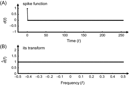
This is the limiting case of an indefinitely narrow Normal function (see Equation 6.27).

The Dirac function, being “infinitely spiky,” has a transform that contains all frequencies in equal proportions. The transform with a spike at t = t₀, is

$\tilde{d}(\omega )={\int }_{-\infty }^{+\infty }\delta (t-t_0)\text{exp}(-i\omega t)\text{d}t={\text{exp}(-i\omega t)|}_{t=t_0}=\text{exp}(-i\omega t_0)$

Although it is an oscillatory function of time, its power spectral density is constant: $s(\omega )={\tilde{d}}^{*}(\omega )\tilde{d}(\omega )=exp(+i\omega t_0)exp(-i\omega t_0)=1$.

The Dirac function can appear in a function's Fourier transform as well. The transform of cos(ω₀t) is

$\tilde{d}(\omega )=\pi (\delta (\omega -{\omega }_0)+\delta (\omega +{\omega }_0))$

This formula can be verified by inserting it into the inverse transform:

$\begin{array}{ll}d(t)\hfill & =\frac{1}{2\pi }{\int }_{-\infty }^{+\infty }\pi (\delta (\omega -{\omega }_0)+\delta (\omega +{\omega }_0))exp(i\omega t)\text{d}\omega \hfill \\ \hfill & =\frac{exp(i{\omega }_{0}t)+exp(-i{\omega }_{0}t)}{2}=\text{cos}({\omega }_{0}t)\hfill \end{array}$

As one might expect, the transform of the pure sinusoid, cos(ω₀t), contains only two frequencies, ±ω₀.

6.7 Area under a function

The area, A, under a function, d(t), is its Fourier transform evaluated at zero frequency; that is, $A=\tilde{d}(\omega =0)$:

$\tilde{d}(\omega =0)={\int }_{-\infty }^{+\infty }d(t)\text{exp}(0)\text{d}t={\int }_{-\infty }^{+\infty }d(t)\text{d}t=A$

as exp(0) = 1. In MatLab, the area is computed as (Figure 6.7)

dt=fft(d);
area = real(dt(1));

(MatLab eda06_08)

6.8 Time-delayed function

Multiplying the transform, $\tilde{d}(\omega )$, by the factor, exp(−iωt₀), time-delays the function by a time interval, t₀:

$\begin{array}{ll}{\tilde{d}}_{\text{delayed}}(\omega )\hfill & ={\int }_{-\infty }^{+\infty }d(t-t_0)\text{exp}(-i\omega t)\text{d}t={\int }_{-\infty }^{+\infty }d(t\text{'})\text{exp}(-i\omega (t\text{'}+t_0))\text{d}t\text{'}\hfill \\ \hfill & =exp(-i\omega t_0){\int }_{-\infty }^{+\infty }d(t\text{'})exp(-i\omega t\text{'})\text{d}t\text{'}=exp(-i\omega t_0)\tilde{d}(\omega )\hfill \end{array}$

Here, we use the transformation of variables, t′ = t − t₀, noting that dt′ = dt and that t′→ ± ∞ as t′→ ± ∞. In the literature, the process of modifying a Fourier transform by multiplication with a factor, $exp(-i\omega t_0)$, is sometimes referred to as introducing a phase ramp, as it changes the phase by an amount proportional to frequency (i.e., by a ramp-shaped function):

$\phi (\omega )=\omega t_0$

The time-shift result appeared previously, when we were calculating the transform of a time-delayed spike (Equation 6.31). The transform of the time-shifted spike differed from the transform of a spike at time zero by a factor of exp(−iωt₀). In MatLab, the time delay is accomplished as follows (Figure 6.8).:

t0 = t(16);
ds=ifft(exp(−i*w*t0).*fft(d));

(MatLab eda06_09)

where t0 is the delay. Note that the symbol i is being used as the imaginary unit. This is the MatLab default, but one must be careful not to reset its value to something else, for example, by using it as a counter in a for loop (see Note 1.1).

6.9 Derivative of a function

Multiplying the transform, $\tilde{d}(\omega )$, by the factor, ιω, computes the transform of the derivative, dd/dt:

$\begin{array}{ll}{\int }_{-\infty }^{+\infty }\frac{\text{d}d}{\text{d}t}\text{exp}(-i\omega t)\text{d}t\hfill & ={d(t)\text{exp}(-i\omega t)|}_{-\infty }^{+\infty }-(-i\omega ){\int }_{-\infty }^{+\infty }d(t)exp(-i\omega t)\text{d}t\hfill \\ \hfill & =0+(i\omega )\tilde{d}(\omega )=i\omega \tilde{d}(\omega )\hfill \end{array}$

Here, we have used integrations by parts, ∫udv = uv−∫vdu, together with the limit, exp(−iωt) → 0 as t → ±∞. In MatLab, the derivative can be computed as follows (Figure 6.9):

dddt = ifft(i*w.*fft(d));

(MatLab eda06_10)

6.10 Integral of a function

Dividing the transform, $\tilde{d}(\omega )$, by the factor, ιω, computes the transform of the integral, ∫d(t) dt:

$\begin{array}{c}{\int }_{-\infty }^{+\infty }{\int }_0^{\text{t}}d(t\text{'})d\text{t}\text{'}\text{exp}(-i\omega t)\text{d}t={\int }_0^{t}d(t\text{'})\text{d}t\text{'}\frac{\text{exp}(-i\omega t)}{-i\omega }{|}_{-\infty }^{+\infty }-\frac{1}{-i\omega }{\int }_{-\infty }^{+\infty }d(t)exp(-i\omega t)\text{d}t\\ =0+\frac{1}{i\omega }\tilde{d}(\omega )=\frac{1}{i\omega }\tilde{d}(\omega )\end{array}$

Here, we have used integrations by parts, ∫udv = uv−∫vdu together with the limit, exp(−iωt) → 0 as t→ ± ∞. Note, however, that the zero-frequency value is undefined (as 1/0 is undefined). As shown in Equation (6.34), this value is the total area under the curve, so it functions as integration constant and must be set to an appropriate value. In MatLab, with the zero-frequency value set to zero, the integral is calculated as follows (Figure 6.10):

integral=ifft(−i*fft(d).*[0,1./w(2:N)′]′);

(MatLab eda06_11)

6.11 Convolution

Finally, we derive a result that pertains to the convolution operation, which will be developed further and utilized heavily in subsequent chapters. Given two functions, f(t) and g(t), their convolution (written f*g) is defined as

$f(t)*g(t)={\int }_{-\infty }^{+\infty }f(\tau )g(t-\tau )\text{d}\tau$

The transform of the convolution is

$\begin{array}{ll}{\int }_{-\infty }^{-\infty }{\int }_{-\infty }^{+\infty }f(\tau )g(t-\tau )\text{d}\tau exp(-i\omega t)dt\hfill & =\hfill \\ \hfill & ={\int }_{-\infty }^{-\infty }f(\tau ){\int }_{-\infty }^{+\infty }g(t-\tau )exp(-i\omega t)dt\text{d}\tau \hfill \\ \hfill & ={\int }_{-\infty }^{-\infty }f(\tau ){\int }_{-\infty }^{+\infty }g(t\text{'})exp(-i\omega (t\text{'}+\tau ))dt\text{'}\text{d}\tau \hfill \\ \hfill & ={\int }_{-\infty }^{-\infty }f(\tau )exp(-i\omega \tau )\text{d}\tau {\int }_{-\infty }^{+\infty }g(t\text{'})exp(-i\omega t\text{'})dt\text{'}\hfill \\ \hfill & =\tilde{f}(\omega )\tilde{g}(\omega )\hfill \end{array}$

Here, we have used the transformation of variables, t′ = t − τ. Thus, the transform of the convolution of two functions is the product of their transforms.

Crib Sheet 6.2

Exemplary pairs of time series d(t) and its amplitude spectral density s(f) (MatLab script eda06_12)

6.12 Nontransient signals

Previously, in developing the relationship between the Fourier integral and its discrete analog, we assumed that the function of interest, d(t), was zero outside of the time window of observation. Only transient signals have this property; we can theoretically record the whole phenomenon, as it lasts only for a finite time. An equally common scenario is one in which the data represent just a portion of an indefinitely long phenomenon that has no well-defined beginning or end. Both the Neuse River Hydrograph and Black Rock Forest temperature datasets are of this type.

Many nontransient signals do not vary dramatically in overall pattern from one time window of observation to another (meaning that their statistical properties are stationary; that is, constant with time). One parameter that is independent of the window length is the power, P:

$P=\frac{1}{T}\int {[d(t)]}^2\text{d}t\approx \frac{\Delta t}{N\Delta t}\sum _{i=1}^N{[d_i(t)]}^2=\frac{1}{N}{\mathbf{d}}^{\text{T}}\mathbf{d}$

In some cases, such as when d(t) represents velocity, P literally is power, that is energy per unit time. Usually, however, the word is understood in the more abstract sense to mean the overall size of a signal that is fluctuating about zero. Note that when the data have zero mean, P = N⁻¹d^Td is the formula for the variance of d. In this special case, the power is equivalent to the variance of the signal, d(t).

The power in a time series has a close relationship to its power spectral density. A time series is related to its Fourier transform by the linear rule, d = Gm, where m is a column vector of Fourier amplitudes. If we were to use the sines and cosines representation of the Fourier transform, then the matrix, G, is given in Equation (6.13). Substituting d = Gm into Equation (6.41) yields

$P=\frac{1}{N}{\mathbf{d}}^{\text{T}}\mathbf{d}=\frac{1}{N}{(\mathbf{G}m)}^{\text{T}}(\mathbf{G}m)=\frac{1}{N}{\mathbf{m}}^{\text{T}}[{\mathbf{G}}^{\text{T}}\mathbf{G}]\mathbf{m}$

However, according to Equation (6.14), G^TG = (N/2)I (except for the first and last coefficient, which we shall ignore). Hence,

$P=\frac{1}{N}\frac{\text{N}}{2}{\mathbf{m}}^{\text{T}}\mathbf{m}=\frac{1}{2}\sum _{i=1}^{\frac{N}{2}+1}(A_i^2+B_i^2)=\frac{1}{2}\sum _{i=1}^{\frac{N}{2}+1}\frac{4}{N^2}{\left|C_i\right|}^2=\frac{2}{{(\Delta t)}^2{N}^2\Delta f}\underset{0}{\overset{f_{ny}}{\int }}{\left|\tilde{d}(f)\right|}^2\text{d}f$

This result is called Parseval's Theorem. Here, the As and Bs are the coefficients in the cosines and sines representation of the Fourier series (Equation 6.13) and the Cs are the coefficients of the MatLab's version of the DFT (Equation 6.21b). The two representations are related by (2/N)C_i = A_i − iB_i. The Fourier transform is approximately, $\tilde{d}(f)=\Delta t{C}_i$. If we define the power spectral density, s²(f), of a nontransient signal as

$s^2(f)=\frac{2}{T}{\left|\tilde{d}(f)\right|}^2\text{then}P={\int }_0^{f_{ny}}{s}^2(f)\text{d}f$

Here, we have used the relations T = NΔt and ΔtΔf = N⁻¹ to reduce 2/[(Δt)²N²Δf] to 2/T. The power is the integral of the power spectral density from zero frequency to the Nyquist frequency. In MatLab, the power spectral density is computed as follows:

tmax=N*Dt;
C=fft(d);
dbar=Dt*C;
thepsd = (2/tmax) * abs(dbar(1:Nf)).○2;

(MatLab eda06_13)

and the total power (variance) is:

P = Df * sum(thepsd);

(MatLab eda06_13)

Here, the data, d, are presumed to have sampling interval, Dt, and length, N.

This simple generalization of the idea of spectral density is closely connected to the limitation that we cannot take the Fourier transform of the whole phenomenon, for it is indefinitely long, but only a portion of it. Nevertheless, we would like for our results to be relatively insensitive to the length of the time window. The factor of 1/T in Equation (6.44) normalizes for window length.

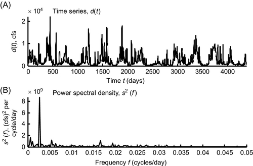
Suppose the units of d(t) are u. Then, the Fourier transform, $\tilde{d}(\omega )$, has units of u-s and the power spectral density has units of u²s²/s = u²s = u²/Hz. For example, for discharge data with units of cubic feet per second, u = ft³/s, and power spectral density has units of ft³, or ft³/s Hz⁻¹ (in the Neuse river hydrograph shown in Figure 6.11, we use the mixed units of ft³/s per cycle/day).

The amplitude spectral density has units of the square root of the power spectral density; that is, u Hz^−1/2.

We have yet to discuss two important elements of working with spectra: First, we have made no mention of confidence limits, yet these are important in determining whether an observed periodicity (i.e., an observed spectral peak) is statistically significant. The reason we have omitted it so far is that the power spectral density is not a linear function of the model parameters, but instead depends on the sum of squares of the model parameters. We lack the tools to propagate error between the data and results in this case. Second, we have made no mention of the tapering process that is often used to prepare data before computing its Fourier transform. We will address these important issues in Chapters 12 and 9, respectively.

Problems

6.1. Write a MatLab script that uses the fft() function to differentiate the Neuse River Hydrograph dataset. Plot the results.

6.2. What is the Fourier transform of sin(ω₀t)? Compare it to the transform of cos(ω₀t).

6.3. The MatLab script, eda06_15, creates a file, noise.txt, containing normally distributed random time series, d(t), with zero mean and unit variance. (A) Compute and plot the power spectral density of this time series. (B) Create a second time series, a(t), that is a moving window average of d(t); that is, each point in a(t) is the average of, say L, neighboring points in d(t). (C) Compute and plot the power spectral density of a(t) for a suite of values of L. Comment on the results.

6.4. Suppose that you needed to compute the DFT of the function

$d(t)=\text{exp}\left(-\frac{t^2}{2{\sigma }^2}\right)$

using MatLab's fft() function. This function is centered on t = 0, and therefore has nonnegligible values for points to the left of the origin. Unfortunately, we have defined the time and data column-vectors, t and d, to start at time zero, so there seems to be no place to put these data values. One solution to this problem is to shift the function to the center of the time window, say by an amount, t₀, compute its Fourier transform, and then multiply the transform by a phase factor, exp(iωt₀), that shifts it back. Another solution relies on the fact that, in discrete transforms, both time and frequency suffer from aliasing. Just as the last frequencies in the transform were large positive frequencies and small negative frequencies, the last points in the time series are simultaneously

$\begin{array}{c}\mathbf{t}={[\begin{array}{cccc}\mathrm{\dots }& (N-3)\Delta t& (N-2)\Delta t& (N-1)\Delta t\end{array}]}^{\text{T}}\\ \text{and}\\ \mathbf{t}={[\begin{array}{cccc}\dots & -3\Delta t& -2\Delta t& -\Delta t\end{array}]}^{\text{T}}\end{array}$

Therefore, one simply puts the negative part of d(t) at the right-hand end of d. Write a MatLab script to try both methods and check that they agree.

6.5. Compute and plot the amplitude spectral density of a cleaned version of the Black Rock Forest temperature dataset. (A) What are its units? (B) Interpret the periods of any spectral peaks that you find.