
Symbols and notations
Sensors operate at the boundary of two physical domains. Despite international normalization of symbols for quantities and material properties, notations for physical quantities are not unambiguous when considering the various disciplines, which each have their own system of notation. This appendix offers a brief review of quantities in the electrical, thermal, mechanical and optical domains, together with their symbols and units, as used in this book. Further, where useful, relations between quantities are listed as well.
A.1 The electrical domain
A sensor produces an electrical output. Table A.1 displays the most important energetic quantities used in the electrical domain. The table also shows magnetic quantities, since they are closely connected to electrical quantities. Relations between these variables are discussed in Chapter 6, Inductive and magnetic sensors.
Table A.1
Table A.2 shows the major properties for the electrical domain.
Table A.2
Conductivity is the inverse of resistivity, and conductance the inverse of resistance. The electric permittivity ε is the product of the permittivity of free space (vacuum) ε0 and the relative permittivity (or dielectric constant) εr. Similarly, the magnetic permeability μ is the product of the magnetic permeability of vacuum μ0 and the relative permeability μr. Numerical values of ε0 and μ0 are:
The relative permittivity and permeability account for the dielectric and magnetic properties of a material.
In the electrical domain, some particular variables apply, associated to properties of (electrical) time-varying signals. They are listed in Table A.3.
Table A.3
| Signal quantity | Symbol | Unit |
|---|---|---|
| Time | t | s (second) |
| Frequency | f | Hz (hertz) = s−1 |
| Period | T | s |
| Phase difference | φ | rad (radian) |
| Duty cycle | δ | – |
| Pulse width | τ | s |
The duty cycle is defined as the high–low ratio of one period in a periodic pulse signal. It varies from 0% (whole period low) to 100% (whole period high). A duty cycle of 50% refers to a symmetric square wave signal.
A.2 The thermal domain
Sensor systems suffer most from unwanted thermal influences. Changes in environmental or local temperature affect the mechanical and electrical performance of mechatronic systems. Therefore we will consider thermal effects when discussing the sensor properties. Tables A.4 and A.5 review the major thermal quantities.
Table A.4
| Energetic quantity | Symbol | Unit |
|---|---|---|
| (Thermodynamic) temperature | Θ | K (kelvin) |
| Quantity of heat | Qth | J (joule) |
| Heat flow rate | Φth | W (watt) |
Table A.5
The coefficient of heat transfer accounts for the heat flow across the boundary area of an object whose temperature is different from that of its (fluidic) environment. Its value strongly depends on the flow type along the object and the surface properties.
A.3 The mechanical domain
Quantities in the mechanical domain describe state properties related to distance, force and motion. A possible categorization of these quantities is divided into:
We will briefly resume the first two groups. Flow quantities are not further discussed in this book. The basic position quantities and their units and symbols are listed in Table A.6.
Table A.6
| Quantity | Symbol | Unit | Relation |
|---|---|---|---|
| Length | l | m | |
| Velocity | v | m/s | v = dx/dt |
| Acceleration | a | m/s2 | a = dv/dt |
| Surface area | A | m2 | |
| Volume | V | m3 | |
| Angular displacement | φ | rad | |
| Angular velocity | ω | rad/s | ω = dφ/dt |
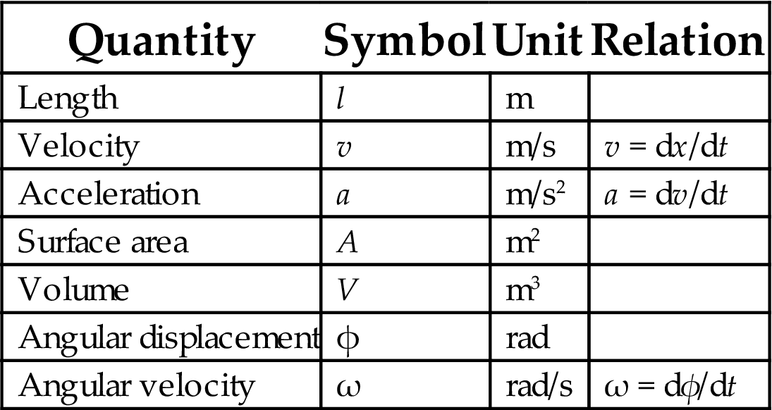
Table A.7 shows the most common force quantities, symbols and units.
Table A.7
| Quantity | Symbol | Unit |
|---|---|---|
| Force | F | N |
| Tension, stress | T | Pa = N/m2 |
| Shear stress | τ | Pa |
| Pressure | p | Pa |
| Moment of force | M | Nm |
| Power | P | W = J/s |
| Energy | E | J = Nm |
Some commonly used properties in the mechanical domain are listed in Table A.8.
Table A.8
| Property | Symbol | Unit | Relation |
|---|---|---|---|
| Mass density | ρ | kg/m3 | M = ρV |
| Mass | M | kg | F = Ma |
| Weight | G | kg | F = Gg |
| Elasticity | c | N/m2 | T = cS |
| Compliance | s | m2/N | s = 1/c |

The relation between tension T and strain S is given by Hooke’s law:
(A.1)
or
(A.2)
Note that compliancy s is the reciprocal of the elasticity c. A force (tension) results in a deformation (strain): longitudinal forces cause translational deformation; shear forces cause rotational deformation; the angle of rotation is called the shear angle. The mechanical domain has six degrees of freedom (d.o.f.): three for translation and three for rotation. As an example, in Fig. A.1 a longitudinal force in z-direction (left) and a shear force around the x-direction (right) are shown. Note that in this example the force causes a positive strain in z-direction and negative strain in the other two directions. The shear force in this example causes only a shear strain in the yz plane; the shear angle is denoted by γ.

In general, a longitudinal force in the z-direction, Tz, causes the material to be deformed in three possible directions (x, y, and z), resulting in the strain components Sz (usually the most important), Sx and Sy. A shear force in the z-plane, Txy, can cause the material to twist in three directions, resulting in the three torsion components Sxy (usually the most important), Sxz and Syz. Sometimes a longitudinal force produces torsion. This can be described by, for instance, Syz=syzz·Tz. In general, the relation between tension and strain is described by
(A.3)
or
(A.4)
with i, j, k, l equal to x, y, and z. Note that for notation symmetry, longitudinal tension Ti (i=x, y, z) is written as Tii. To simplify the notation the tensor indices ijkl are substituted by engineering indices 1–6, according to the next scheme:
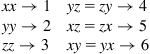
So, Hooke’s law becomes:
(A.5)
or
(A.6)
with λ, μ=1 … 6. Apparently this compliance matrix contains 36 elements. Written in full
(A.7)
 (A.7)
(A.7)In most materials many of the matrix elements in Eq. (A.7) are zero, due to symmetry in the material crystal structure. To get an idea of the practical values Table A.9 shows numerical values of the elements of the compliance matrix of quartz (crystalline SiO2) and of silicon (Si). Note that sij=sji. Silicon has an almost symmetrical crystal structure, leading to s11=s22=s33, s44=s55=s66 and s12=s13. The remaining elements in the matrix are zero. Obviously quartz has a less symmetrical structure, as can be deduced from the many different element values.

A.4 The optical domain
A.4.1 Optical quantities
In the optical domain two groups of quantities are distinguished: radiometric and photometric quantities. The radiometric quantities are valid for the whole electromagnetic spectrum. Photometric quantities are only valid within the visible part of the spectrum (0.35<λ<0.77 μm). They are related to the mean, standardized sensitivity of the human eye and are applied in photometry. Table A.10 shows the major radiometric and corresponding photometric quantities. Some of them will be explained in more detail.
Table A.10
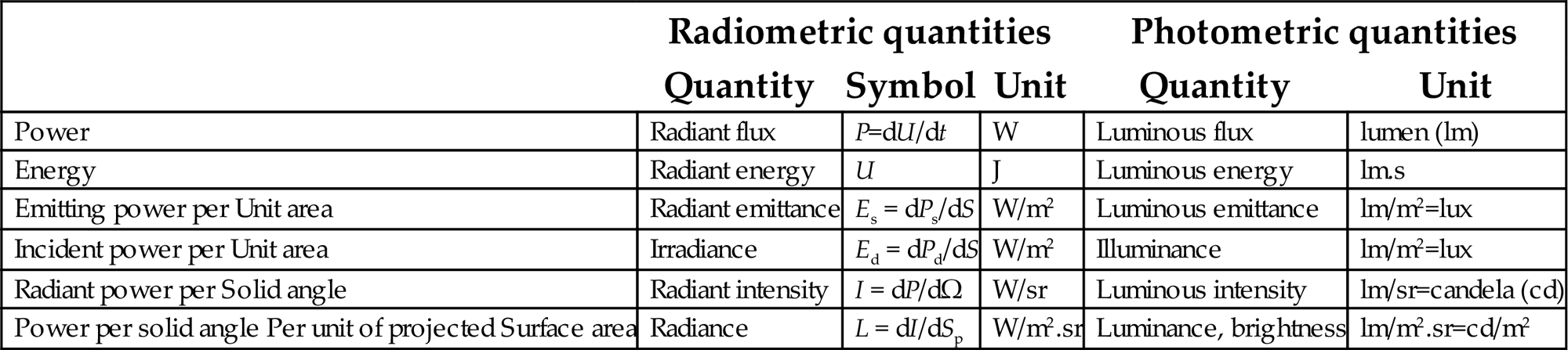
The radiant intensity I (W/sr) is the emitted radiant power of a point source per unit of solid angle. For a source consisting of a flat radiant surface the emitted power is expressed in terms of W/m2, called the radiant emittance Es. It includes the total emitted energy in all directions. The quantity radiance also accounts for the direction of the emitted light: it is the emitted power per unit area, per unit of solid angle (W/m2 sr).
A flat surface can receive radiant energy from its environment, from all directions. The amount of incident power Ed is expressed in terms of W/m2 and is called the irradiance.
In radiometry the unit of (emitting or receiving) surface area is often expressed in terms of ‘projected area’. A surface with (real) area S that is irradiated from a direction perpendicular to its surface receives power equal to Ed·S (W). When that surface is rotated over an angle ϕ, relative to the direction of radiation, it receives only an amount of radiant power equal to Ed·S·cos ϕ (Fig. A.2). To make these radiometric quantities independent of the viewing direction, some authors express them in terms of projected area instead of real area, thus avoiding the cosϕ in the expressions.

In Table A.10 the radiance L of a surface is defined following this idea: it is the emitted radiant energy in a certain direction, per solid angle (to account for the directivity) and per unit of projected area, that is per unit area when the emitting surface is projected into that direction. These quantities are used for deriving formulas for sensors that are based on reflecting surfaces (Chapter 7: Optical sensors).
All units have their counterpart in the photometric domain (right-hand side of the table). However, we will not use them further in this book. The radiometric quantities in the table do not account for the frequency or wavelength dependence. All of them can be expressed also in spectral units, e.g., the spectral irradiance Ed(λ), which is the irradiance per unit of wavelength interval (W/m2 μm). The total irradiance over a spectral range from λ1 to λ2 then becomes:
(A.8)
To characterize optical sensors special signal parameters are used, related to the noise behavior of these components (Table A.11).
Table A.11
Note that the signals can be expressed in voltage, current or power. Irrespective of this choice, the S/N ratio is a dimensionless quantity. The parameters D and NEP represent the lowest perceivable optical signal. NEP is, in words, equal to the power of sinusoidally modulated monochromatic radiation that produces an RMS signal at the output of an ideal sensor, equal to the noise signal of the real sensor. This means that, when specifying NEP, the modulation frequency, the sensor bandwidth, the temperature and the sensitive surface area should also be specified, as all these parameters are included in the noise specification. To avoid wavelength and detector area dependency in the specifications, the parameters NEP* and D* are used: the spectral NEP and the spectral D, respectively. Since noise power of a sensor is usually proportional to the sensitive area A and the bandwidth Δf, the noise current and noise voltage are proportional to √(AΔf); hence, NEP*=NEP/√(AΔf) and D*=√(AΔf)/NEP.
A.4.2 Radiant energy from a unit surface with Lambertian emission
If a surface is a perfect diffuser (its radiance is not a function of angle), then I=I0·cos ϕ (Fig. A.3).

This is known as the cosine law of Lambert. Many surfaces scatter the incident light in all directions equally. A surface that satisfies Lambert’s law is called Lambertian.
All radiant energy emitted from a surface A with radiant emittance Es has to pass a hemisphere around that surface (Fig. A.4).

The area of surface element dS on the hemisphere, corresponding with a solid angle dΩ equals:
(A.9)
where r is the radius of the hemisphere. According to its definition in Table A.10 the radiant emittance from the emitting surface A in the direction of dS is:
(A.10)
Since all radiant energy from A passes the hemisphere, the total radiant emittance of A equals the integral of dPs/dA over the full surface area of the hemisphere. Further, since for a Lambertian surface the radiant emittance is independent of the direction, L is constant. So
(A.11)
or the radiant emittance of a Lambertian surface equals π times the radiance of that surface.
A.4.3 Derivation of relations between intensity and distance
The transfer characteristic of an optical displacement sensor (Chapter 7: Optical sensors) depends strongly on the geometry of the configuration. Fig. A.5 depicts the major parameters involved in the direct mode.

Light energy radiates from the source with emitting surface area S1 and radiance Le (W/sr m2). The sensor surface area is S2, the distance from source to sensor is r. Further, the light beam as received by the sensor makes an angle ϑ1 with the normal on the emitting surface, and an angle ϑ2 with the normal on the receiving surface. We calculate the radiant power that arrives at the sensor. Assume the source dimensions being small compared to r. Then the light beam that arrives at the sensor has a solid angle equal to
(A.12)
where S2 cos ϑ2 is the projected surface area of the sensor. The emitter emits Le·S1 W per steradian; hence, the part ΔPe of the emitted light falling on the sensor is:
(A.13)
where S1 cos ϑ1 is the projected surface area of the source. By substituting Eq. (A.13) in Eq. (A.12) we find for the radiant power arriving at the sensor:
(A.14)
from which follows that the output signal, indeed, is inversely proportional to the square of the distance.
Next we consider the indirect mode, where we distinguish between two different situations. In the first situation the reflecting target is only partly illuminated by the source; all the light from the source is intercepted by the object. In the second situation the whole object falls within the light cone of the source. Fig. A.6 displays the first situation and defines the various parameters. For a better understanding, the object (target) is presented twice, once as the receiving surface and once as the (secondary) emitting surface.

The target intercepts a light beam that makes an angle ϑs with the normal vector nt on the target’s surface. The source can be characterized by an intensity Is (W/sr) and a beam solid angle Ωs. The surface area S1 of the light spot on the object satisfies the equation:
(A.15)
where rs is the distance between the source and the target. The irradiance of the object (actually the lighted part of it) is:
(A.16)
Since the object surface is assumed to be Lambertian it behaves as a radiant source with radiance L1=E1/π (see Eq. (A.11)). Part of the scattered light is received by the detector with sensitive area Sd on a distance rd from the target. Similar to Eq. (A.12) this sensor receives light over a solid angle Ωd equal to
(A.17)
The radiant power received by the sensor is:
(A.18)
Finally, when substituting Eqs (A.16) and (A.17) into Eq. (A.18) we find for the optical power received by the sensor:
(A.19)
So the sensor output is inversely proportional to the square of the distance to the sensor, as long as the object intercepts the whole light beam. Note that Pd does not depend on the angle ϑs, because all the light from the source falls on the object, whose surface is assumed to be Lambertian.
Next we consider the situation where the whole object is illuminated by the source, as can happen at large distances and with small objects (Fig. A.7).

The solid angle of the beam falling on the object is:
(A.20)
where St is the area of the illuminated part of the object. The radiant emittance now becomes:
(A.21)
Following the same steps as before, we find for the radiant power received by the sensor:
(A.22)
Clearly the sensor output is inversely proportional to the fourth power of the distance between source/sensor and the target.