
Acoustic sensors
Abstract
The chapter opens with an overview of acoustic parameters and properties. Next the operation and performance of piezoelectric and electrostatic transducers are discussed. In the ensuing section various methods for distance measurements are given, generally based on the ToF principle. Finally, in the application section, we discuss examples of ranging and imaging, as well as nondestructive testing, inspection using acoustic principles and interfacing.
Keywords
Acoustic properties; sound propagation; acoustic impedance; electrostatic transducers, piezoelectric transducers; directivity; ToF distance measurement; navigation; NDT; interfacing
The primary measurand of an acoustic sensor is sound intensity. In combination with a controllable sound source, acoustic sensors can be used for measuring various other physical parameters, e.g., distance, velocity of fluids, material properties, chemical composition, and many more. They are also suitable for navigation (of mobile robots), imaging (e.g., rangefinding and object recognition) and quality testing. In mechatronics they mainly fulfill the task of noncontact measurement of distances and derived quantities. Similar to optical sensing systems, such acoustic sensing systems also comprise basically three parts: a source, a receiver, and a modulating medium (in mechatronics the medium is mostly air). Many acoustic sensing systems are based on the measurement of the travel time or ToF, that is the time it takes for an acoustic wave or signal to travel a certain path
(9.1)
This path is made dependent on the physical parameter to be determined, e.g., a distance. Such a time-based measurement approach is preferred over intensity-based measurements, because the latter are less accurate and the relation between distance and intensity is often affected by unpredictable sound reflections and scattering.
Acoustic sensing has some advantages over optical sensing:
We start the chapter with an overview of acoustic parameters and properties. Next the operation and performance of some acoustic (ultrasonic) sensors are discussed. In the ensuing section various methods for contact-free distance measurements are given. Finally, in the application section, we discuss examples of ranging, imaging, and interfacing.
9.1 Properties of the acoustic medium
Unlike light (electromagnetic waves) that can propagate in a vacuum, sound waves need an elastic medium to travel. The most common waves are longitudinal waves and shear waves. In longitudinal waves the particle motion is in the same direction as the propagation; in shear waves the motion is perpendicular to the propagation direction. Some sensors utilize surface acoustic waves (SAWs). An absorbing substance is deposited on the surface of a device on which the waves are travelling: The SAW's velocity is influenced by the concentration of the absorbed matter. Such SAW devices are suitable for chemical sensing. The selectivity is greatly determined by the chemical interface.
In this chapter we only discuss acoustic sensors for the measurement of mechanical quantities in mechatronics, where the propagation medium is generally air. Since the quality of an acoustic measurement strongly depends on the acoustic properties of the medium, we present here an overview of the major acoustic characteristics of air. But first we give some definitions of terms commonly in use in acoustics.
9.1.1 Sound intensity and pressure
Any piece of vibrating material radiates acoustic energy. The rate at which this energy is radiating is called the acoustical or sound power (W). Sound intensity is the rate of energy flow through a unit surface area; hence intensity is expressed as W/m2 (compare the optical quantity flux). A sound wave is characterized by two parameters: the sound pressure (a scalar, the local pressure changes with respect to ambient) and the particle velocity (a vector). The intensity is the time-averaged product of these two parameters. It may vary from zero (when the two signals are 90 degrees out of phase) to a maximum (at in-phase signals). The relation between intensity and pressure in the free field (no reflections) is simply given by the equation
(9.2)
where p is the pressure (in root-mean-square or RMS value), ρ the density, and v the speed of sound. This equation is only valid in a free field.
Often sound power, pressure, and intensity are expressed in dB, which means relative to a reference value. Common reference values are: Pref=1 pW, Iref=1 pW/m2, and pref (threshold of hearing) about 20 μPa.
For example for the intensity at 2 m away from a sound source of P=1 mW at the ground, the surface area of the hemisphere is about 25 m2 (half of 4πr2), so the intensity in dB amounts 10 log(I/Iref)=76 dB.
In the free field pressure and intensity levels are numerically the same (when using the same references), but in practice there is a difference between these two levels. Most sensors do not measure sound intensity, but sound pressure only. Note that for a sine wave (a pure sound tone), the RMS pressure is ½√2 times the pressure amplitude, similar to the case of electrical signals.
9.1.2 Sound propagation speed
In general the propagation speed of sound in a material is given by the equation
(9.3)
where c is the stiffness (modulus of elasticity) and ρ the specific mass of that material. For ideal gases the expression for the speed of sound is:
(9.4)
where Θ is the absolute temperature, R the gas constant, and M the molecular mass. Substitution of numerical values for air yields:
(9.5)
with ϑ the temperature in °C. Hence, as a rule of thumb, the temperature coefficient of va is about 2% per 10 K. The influence of air humidity is relatively small and is only relevant when high accuracy is required.
The speed of sound is roughly 106 times lower than the speed of light. Hence ToF is easier to measure, but consequently the measurement time is longer. Moreover the much larger wavelength of sound waves compared to light waves makes it more difficult to manipulate with sound beams (e.g., focusing or the creation of a narrow beam).
Acoustic velocity differs from particle velocity u. The latter follows from Euler’s equation for the acceleration of a fluid:
(9.6)
for the particle velocity in the x-direction.
9.1.3 Acoustic damping
An acoustic wave is attenuated by molecular absorption of sound energy and by scattering: the wave gradually loses energy when propagating. For a plane wave Beer’s law applies:
(9.7)
Pi is the acoustic power at a certain place x in space, Po is the power at a place Δx farther in the direction of propagation. The attenuation or damping coefficient α comprises two effects: absorption loss and scattering loss. In solids the first effect is proportional to frequency, and the second proportional to the square of the frequency. In gases the second term dominates, hence α=a·f2: the attenuation of the wave increases with squared frequency. Acoustic damping also depends on gas composition. For air it means that acoustic attenuation is affected by the air humidity. Table 9.1 shows some values of damping in dry and humid air.
Table 9.1
| Medium | Frequency (Hz) | α (dB/m) |
|---|---|---|
| Dry air | 106 | 160 |
| 10% RH | 105 | 18 |
| 90% RH | 105 | 42 |
9.1.4 Acoustic impedance
The acoustic impedance is defined as the ratio between the (sinusoidal) acoustic pressure wave p and the particle velocity u in that wave. For a sound wave that propagates only in one direction, the acoustic impedance Z is found to be:
(9.8)
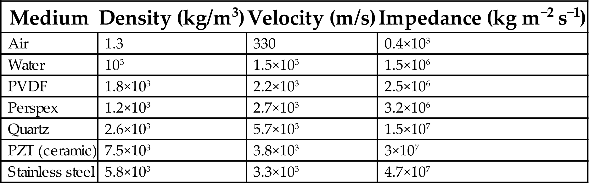
Table 9.2 displays typical values for various materials. Clearly air has a very low acoustic impedance; liquids and solids are much “harder” materials.
Table 9.2
The acoustic impedance is an important parameter with respect to the transfer of acoustic energy between two media. Similar to light waves which show reflection and refraction on the interface of two media with different optical properties (i.e., refractive index, dielectric constant, and conductivity), sound waves are also reflected at the interface of two media with different acoustic properties. When a sound wave arrives at such a boundary, part of the acoustic energy is reflected back and the remaining part enters the other medium. The amount of reflected or transmitted energy can be expressed in terms of the acoustic impedances. For sound waves Snell’s law applies to calculate the direction and amplitude of the refracted sound. In the special case of a wave perpendicular to the boundary plane, the ratio between reflected and incident power (the reflection ratio) is given by
(9.9)
Z1 is the acoustic impedance of the medium of the incident wave, Z2 that of the medium behind the boundary plane. Obviously there is no reflection (hence total transmission) if both media have equal acoustic impedance. On the other hand when the impedances show a strong difference, the power transmission is small.
This has two important consequences for the S/N in ToF measurements where emitter and receiver are both facing the reflecting surface. First an airborne sound wave that arrives at a solid object reflects in the same way as light on a mirror. Waves with an oblique angle of incidence reflect away from the direction of the emitter, so the reflected sound does only partially arrive at the receiver which is usually placed very near the emitter. Secondly, transmission from an acoustic “soft” material to an acoustic “hard” material is poor. This applies in particular for acoustic sensors in air applications because of the wide gap between impedances of air and most sensor materials. Since many systems consist of a source and a detector, the power loss occurs twice, resulting in a low S/N ratio in acoustic sensing systems.
9.2 Acoustic sensors
9.2.1 General properties
Commonly used acoustic sensors belong to one of the following types:
The first two types enjoy great popularity in various ultrasonic applications (frequencies above 20 kHz). The transduction effects are reversible, which means that an acoustic transducer might be used as a source (transmitter) as well as a sensor (receiver). ToF systems may have both a transmitter and a receiver, or only one transducer alternately in use as a transmitter and a receiver.
We will now derive an approximated expression for the spatial distribution of the acoustic power emitted by an ultrasonic transducer. A common model for a transducer, used for this purpose, is the plane piston model: a circular disc vibrating in thickness mode (Fig. 9.1).

Each element dS of the disc surface acts as a point source for acoustic waves. The sound intensity in any point P in the hemisphere around the piston can be calculated by summing all contributions to the pressure variations in that point from each of the point sources dS. At places where the sound waves are (partly) out of phase, the sound intensity is low; at places where the waves are in-phase, the sound intensity is high. This results in an interference pattern of acoustic waves in front of the transducer: the acoustic pressure appears to have peaks and lows in particular directions and at particular distances from the transmitter.
For simplicity we will consider two special cases: The pressure along the main axis of the transducer (φ=0), and the pressure at a distance r far from the center, for arbitrary angle φ.
The acoustic pressure along the main or acoustic axis p(x) is given by [2]
(9.10)
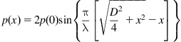 (9.10)
where p(0) is the amplitude of the acoustic pressure on the plate surface (x=0) and x the distance from the plate on the main axis. This is just the result of integrating the contributions to the pressure from all surface patches dS. Fig. 9.2 shows a picture of the relative pressure along the acoustic axis for two cases: D=15 mm, λ=8 mm and D=15 mm, λ=1.5 mm. Close to the emitter the pressure shows strong pressure variations with distance. The place of the last maximum, at distance xM from the plate, is taken as the boundary between the near field (or Fresnel zone) and the far field (or Fraunhofer zone) of the transducer.

Extreme values of p(x) in Eq. (9.10) occur for
(9.11)
The maximum for the largest value of x is found for k=0 and amounts:
(9.12)
At frequencies for which the wavelength is small compared with the dimension of the transmitter, the near field covers a range which is roughly D2/4λ. The typical application example of Fig. 9.2A with D=15 mm, λ=8 mm (40 kHz in air) shows that the near field ranges about 6 mm only. It means that in most mechatronic applications (in particular ToF measurements in air) we only need to consider the propagation in the far field.
An important sensor characteristic is the directivity diagram, representing the sound pattern in the far field. For a circular piston this directivity diagram is rotationally symmetric and can be represented in a plane. Imagine a sphere (or circle) with radius r around the center of the transmitter. The pressure distribution over this sphere can be described by the expression [2, p. 78]
(9.13)
where p(r) is the pressure at distance r, λ the wavelength of the sound signal, D the plate diameter, and J1(πD sin φ/φ) is an order-1 Bessel function. The diagram consists of several “lobes,” a main lobe and side lobes. The width of the main lobe follows from Eq. (9.13). An approximated value for the half angle φh (or angle of divergence or the cone angle) of the main lobe is given by [1, p. 73]
(9.14)
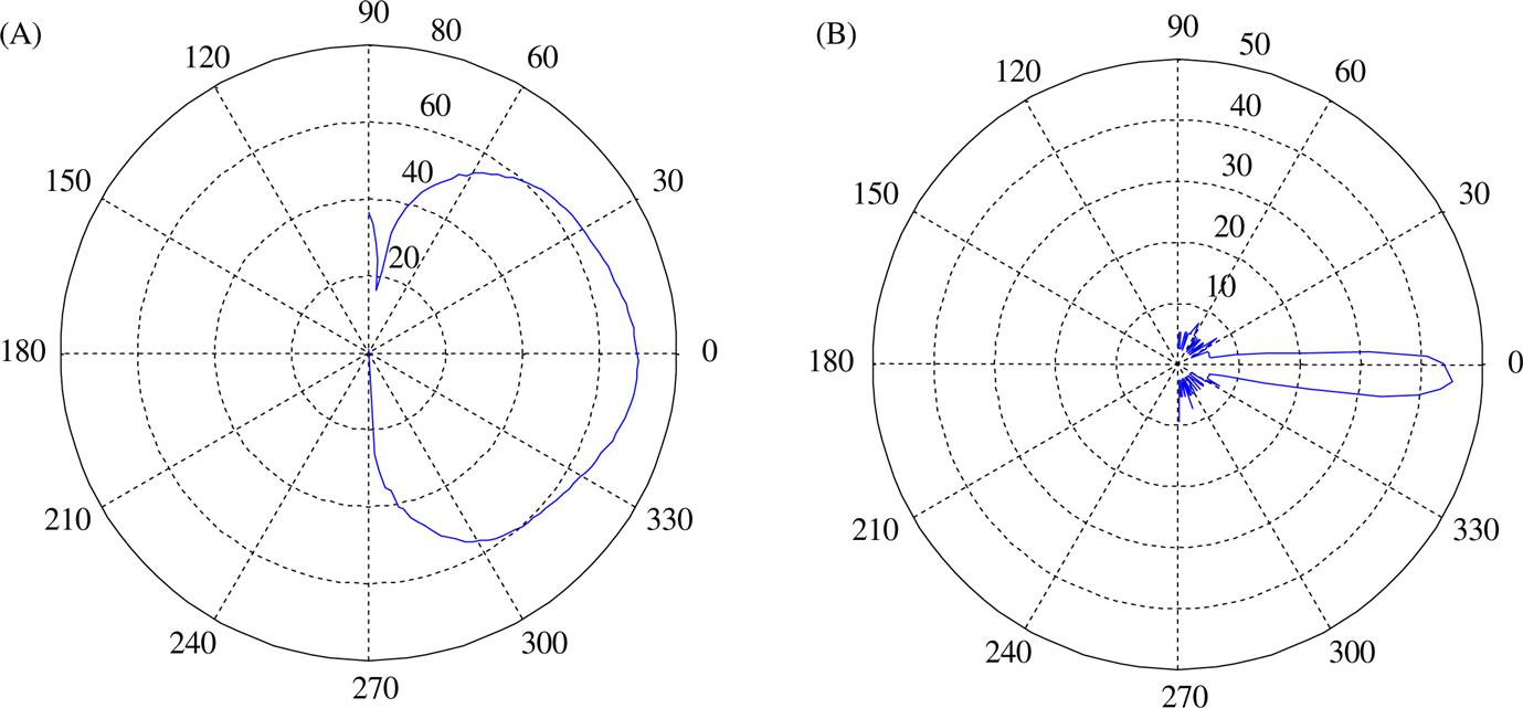
Apparently the ratio D/λ determines the direction selectivity of the transducer: A narrow beam is achieved by a large ratio (D![]() λ). The theoretical directivity diagram derived by Eq. (9.13) is just a very rough approximation, since practical transducers do not behave as a piston. Fig. 9.3 gives the directivity diagram of two real transducers, a piezoelectric and an electrostatic transducer (see Section 9.2).
λ). The theoretical directivity diagram derived by Eq. (9.13) is just a very rough approximation, since practical transducers do not behave as a piston. Fig. 9.3 gives the directivity diagram of two real transducers, a piezoelectric and an electrostatic transducer (see Section 9.2).
The smaller the size of the transducer (characterized by the diameter D), or the larger the wavelength λ, the more it behaves as a point source. For a narrow beam (required for optimal S/N ratio), the transducer should be large compared to the wavelength. This means, to obtain narrow beams, we have to choose either a large transducer (which might be impractical in many applications) or a high frequency (resulting in increased damping and therefore a reduced range).
Since actual transducers may have shapes that differ from the circular piston model, the pressure field patterns have much more complicated shapes; see, e.g., Ref. [3]. By special design the beam angle can be made smaller, resulting in so-called focused probes [2, Chapter 5].
We will now resume the operation principle and properties of two types of acoustic sensors most encountered in mechatronics: the electrostatic and the piezoelectric transducers.
9.2.2 Electrostatic transducers
An electrostatic (or capacitive) ultrasonic transducer consists of two flat conductive plates, one fixed to the housing, the other movable relative to the fixed plate, together constituting a flat-plate capacitor (Fig. 9.4A). For this construction the equations V=Q/C and C=ε0εrA/d apply (see Chapter 5: Capacitive sensors).

In the receiver mode the moving plate is charged with a more or less constant charge, which is realized by connecting the plate via a resistor to a rather high DC voltage of some hundred volts. Sound waves (moving air particles) bring the plate into motion. Due to the constant charge and the changing plate distance, the voltage across the plates varies in accordance with the sound wave. To obtain a high sensitivity the plate is made very thin and flexible, resulting in an enhanced acoustic coupling to the air (see Section 9.1.4 on acoustic impedance). Obviously the sensitivity is also proportional to the DC voltage on the movable plate. The necessity of an external high voltage is the major drawback of the electrostatic transducer.
An alternative to such an external voltage is the electret version in which a charge is permanently stored in a sheet of a suitable piezoelectric material, making up the fixed plate of the capacitor. Such electret (or electret condenser) microphones for air-coupled applications operate mainly in the audible range (20–20 kHz).
In the transmitter mode an AC voltage is put on the movable plate of the capacitor. A voltage difference V between the plates results in a force equal to
(9.15)
with S the surface area of the plates and d the gap distance. Since this electrostatic force (explaining the name of this type of transducer) is proportional to the square of the voltage, it is always contractive, driving the movable plate toward the fixed plate until it is in equilibrium with the counterforce of the elastic bond. Should the plate move linearly proportional to an applied AC voltage (to generate the proper sound waves), the capacitor should be biased with a DC voltage higher than the amplitude of the AC voltage. Eq. (9.15) also shows that the sensitivity of the emitter increases with decreasing initial plate distance.
To make a robust transducer with small initial gap and a thin movable plate (membrane), the latter is sustained not only at its edges, but over a larger part of the surface (Fig. 9.4B), accomplished by, e.g., a grooved plate or other isolating structures like a grid or a net [4]. Obviously the membrane only vibrates at places where it is free to move. This multimode vibration explains the large deviations in the directivity diagrams of real electrostatic transducers as compared to those given in Fig. 9.3. Moreover the layout of the structure strongly determines the frequency characteristics of the transducer [5]. On the other hand it allows designers of electrostatic transducers to optimize transducer characteristics for particular applications.
Like many other sensors ultrasound transducers can also be manufactured using silicon technology. The membrane in such devices is made from silicon by anisotropic etching, similar to the piezoresistive pressure sensors discussed in Chapter 4, Resistive sensors. It acts as the movable (vibrating) electrode of a capacitor-like structure [6,7]. An important advantage of this technology is the ability to make large numbers of membranes on a single chip. Silicon membrane sensors have a smaller bandwidth, due to (multimode) resonance frequencies of the mechanical structure. The output power and sensitivity are substantially less than the macro devices, because of the much smaller dimensions and deflections of the micro membranes.
9.2.3 Piezoelectric transducers
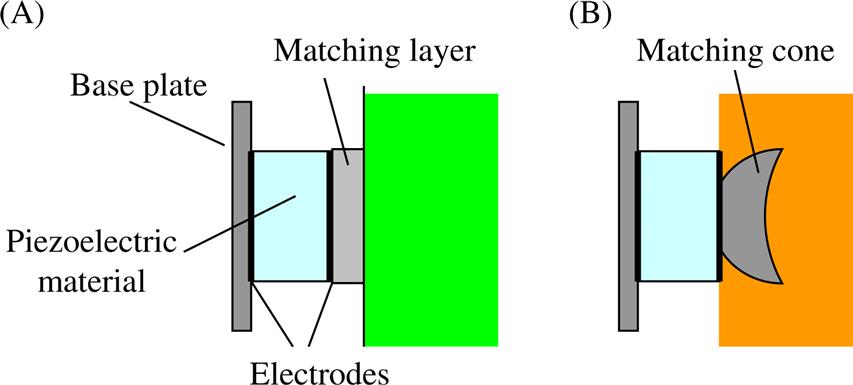
A piezoelectric acoustic transducer consists of a piece of piezoelectric material (Chapter 8: Piezoelectricity), configured as a flat-plate capacitor (Fig. 9.5). An AC voltage applied to the crystal causes the material to vibrate, resulting in the generation of acoustic energy. Conversely when the crystal is deformed by incident sound waves, a piezoelectric voltage is induced. Hence the transducer might be used in transmitter mode and in receiver mode, similar to the electrostatic transducer but without the need of a biasing DC voltage.
Irrespective of the application the transfer of sound energy from transducer to medium or vice versa is crucial for the S/N ratio of the measurement signal. As explained in Section 9.1.4 the transfer is governed by the acoustic impedances of the materials involved. Obviously since a piezoelectric ceramic material has a high acoustic impedance compared to air, the efficiency of power transfer to air is extremely poor. Also for a liquid or solid medium, power loss can be considerable too. In case of a solid, air voids between the transducer and the solid significantly lowers the transmission efficiency, a problem often encountered in acoustic non-destructive testing (NDT) of objects. In such applications a coupling gel between the transducer and the (solid) object under test is essential.
There are many ways to improve the transmission of sound from the transducer to its acoustic environment. However, efficiency is not the only characteristic of interest: Bandwidth and beam shape are equally important parameters. Optimization is often a compromise between these parameters. Advanced models of the acoustic arrangement, based on transmission lines, are required to find an optimal solution for a particular application.
Basically there are two major approaches: matching layers and shaping. The first is usually applied for liquid and solid contacts (Fig. 9.5A). Two essential parameters of such a layer are the acoustic impedance and the thickness. The acoustic impedance of the matching layer should have a value between that of both materials at either side of this layer. According to very simple models, the optimum value is the harmonic mean of these two values, but in practice other values appear to be more effective [2, Chapter 4]. The thickness of the plate should be equal to a quarter of the sound wavelength, to minimize the reflection at the front side of the matching layer, in favor of the transmitted waves. Having found the optimum impedance value, the next problem is finding a material having that particular impedance. Matching layer design is still the subject of continuous research, including the search for suitable materials, the use of multiple matching layers and backing layers, extension of the frequency range and manufacturing issues—e.g., the influence of the glue between the layers [8] and the use of silicon-compatible technologies.
To overcome the enormous mismatch in airborne applications, the transmission efficiency is improved by placing a precisely shaped piece of an acoustically soft material on the front side of the ceramic element, e.g., a tiny horn as shown in Fig. 9.5B. A horn or cone also affects the frequency range as well as the radiation field of the transducer [1, p. 102]. Most commercial low-cost piezoelectric transducers are provided with such a horn.
Poled PVDF has a relatively low acoustic impedance (see Table 9.2), making it an attractive material for ultrasound applications. The flexibility of the material allows operation in bending mode, whereas the ceramic sensors usually operate in thickness mode [9,10]. Other piezoelectric materials are being studied for their suitability as acoustic transducer, e.g., porous films with artificially electric dipoles [11].
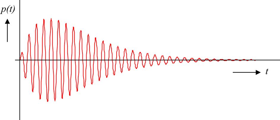
Piezoelectric transducers operate best at resonance: The high stiffness of ceramic materials results in a narrow bandwidth (in other words, a high mechanical Q-factor). The resonance frequency is determined by the dimensions of the crystal, and to a lesser extent by the matching elements. Popular frequencies are 40 and 200 kHz. Many acoustic detection systems use tone burst signals. A typical response of a piezoelectric transducer to a burst signal at the resonance frequency is shown in Fig. 9.6. Apparently the output burst shows strong distortion at the edges, due the narrow bandwidth of the device. This has important consequences for the determination of the ToF measurement, as will be explained in Section 9.3.
9.2.4 Arrays
As shown in Section 9.2.1 the beam width of a sound emitter is determined by its lateral dimensions and the frequency of the emitted sound signal. With a properly designed (linear) array of transducers a much narrower beam can be obtained, using spatial interference of the individual acoustic signals (Fig. 9.7).
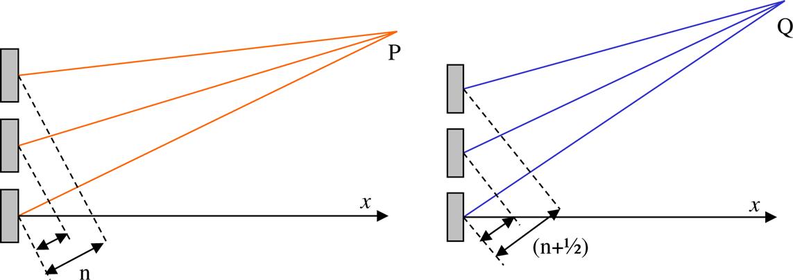
For points in the hemisphere where the travelled distances differ a multiple of the wavelength, the waves add up (e.g., in P). In other points, as in Q, the waves (partly) cancel. Moreover the direction of this beam can be controlled over a limited range (±30 degrees) with the phase difference of the applied electrical signals. Similarly the sensitivity angle of an acoustic transducer operating in receiver mode can be narrowed using an array of such receivers. At the receiving side the individual outputs are added after a properly chosen time delay. By controlling the delay times the main sensitivity axis can be varied over a limited angle. The application of this general principle to acoustic transducers has already been described in earlier literature [12–15]. Due to improved technology phased arrays are gaining interest for acoustic ranging and imaging [16–19]. They eliminate the need for a mechanical (hence slow) scanning mechanism but have a limited angular scanning range. In general at an increasing deflection angle the amplitude of the side lobes (Fig. 9.3) increases as well, deteriorating the beam quality.
9.3 Measurement methods
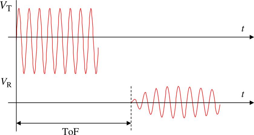
The majority of acoustic distance measurement systems are based on the ToF method. A measurement based on distance-dependent attenuation (as with light) is rather susceptible to environmental influences and the absorption properties of the objects involved. In most acoustic ToF systems the elapsed time between the excitation of a sound pulse and the arrival of its echo is measured (Fig. 9.8). Since the transduction effects are reversible, the transducer can be switched from transmitter to receiver mode, within one measurement. The travelled distance x follows directly from the ToF t, using the relation va=x/t (for direct travel) or va=2x/t for echo systems (where the sound wave travels twice the distance).
The sound signal can be of any shape. Most popular are the burst (a number of periods of a sine wave), a continuous wave with constant frequency (CW), and an FM-modulated sine wave (FMCW or “chirp”). We discuss the major characteristics of these three types. Pulses and bandwidth limited Gaussian noise are other possibilities.
9.3.1 Burst
The tone burst is the most common signal type used for acoustic distance measurements in air, in particular for applications where high accuracy is not required (e.g., ranging, navigation, obstacle avoidance). A transmitter emits a short burst, a few up to about 10 periods of a sine wave, in the direction of an object. The sound reflects (in accordance with the reflection properties of the object’s surface and its orientation, as discussed in Section 9.1), travels back and is received by the same or a second transducer, which detects the moment of arrival.
Due to various causes the accuracy of the ToF measurement—and so the distance measurement—is limited. First there is noise of electrical and acoustic origin, which becomes important at larger distances, when the echo signal is low due to divergence of the sound waves. Next, spurious reflections can also mask the arrival time of the main echo. A further cause of inaccuracy is the (unknown) orientation of the reflecting surface relative to the main axis of the transducers. Finally the narrow bandwidth of a piezoelectric transducer makes the edges of the burst less pronounced, obstructing an accurate detection of the starting point of the pulse. Some but not all of these causes are typical for the burst method.
In case of an individual transmitter and receiver with spacing a (Fig. 9.9A) the measured distance x′ is:
(9.16)
from which follows a relative error equal to
(9.17)

So, for a distance x 3.5 times the space between T and R, the relative error is 1% only, which is acceptable in most practical situations.
A tilted reflecting surface (Fig. 9.9B) introduces a typical cosine error of −α2/2, with α in radians: Only waves normal to the surface will return to the receiver. As an example, a 1% error occurs when the tilt angle is about 8 degrees. Note, however, that the sound intensity is reduced according to the directivity. When in this numerical example the half-angles of both R and T are also 8 degrees, the intensity of the echo has dropped by a factor of four.
When a single transducer is used, switching from transmitter to receiver mode is only possible after the complete burst has been transmitted. This limits the minimum detectable distance: there is a dead band or dead zone, equal to half the number of wavelengths (because sound is travelling twice the distance). Shortening the pulse duration reduces this dead band, but also the sound energy, and hence the S/N ratio is reduced.
The response of a piezoelectric transducer on a burst (Fig. 9.6) shows a rather large rise time due to the high quality factor of this transducer type. Actually this effect occurs twice: First at the transmitter and a second time at the receiver. The starting point of the echo is then easily obscured by noise.
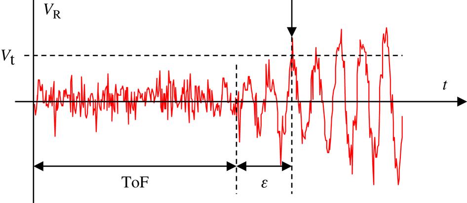
The most common detection method for the echo burst is a threshold applied to the receiver signal. The ToF is set by the first time the echo exceeds the threshold. The threshold must be well above the noise level, to prevent noise being interpreted as the incoming echo. On the other hand when the threshold is too high, one or more periods of the received signal can be missed, as shown in Fig. 9.10. At 40 kHz this results in an error of (a multiple of) about 8 mm, which is the penalty for this simple signal processing scheme.
Many methods have been published over the past years, all aiming at a higher accuracy of the burst ToF measurement, despite noise and other interfering effects such as temperature changes and air turbulence. One such approach is to use the complete echo signal and not just the starting point to determine the ToF, e.g., by autocorrelation or cross correlation [20,21]. These techniques yield typical errors below 1 mm, depending on the S/N ratio and the travelled distance but need longer processing time. Another approach is based on knowledge about the shape of the echo's envelope, which is determined by the transducer’s transfer function [22]. Alternatively instead of the starting point of the echo signal, where the S/N ratio is low, the arrival time of a point around the maximum amplitude could be chosen as a measure for the ToF. With this method the typical distance error can be less than 0.1 mm [23]. Other researchers use the phase information comprised in the echo signal, the typical shape of the envelope, or just more advanced signal processing techniques [24–28]. Noise as the input signal is studied in Ref. [29]. A comparison of various detection methods is presented in Ref. [30].
9.3.2 Continuous sine wave (CW)
The average output power of a burst is relatively small, and may result in a poor S/N ratio, in particular at increased distances. In this respect the emission of a continuous acoustic signal is better. Distance information is obtained from the phase difference between the transmitted and the received waves. This method has two main drawbacks. First emission and detection cannot share the same transducer, hence two transducers are required, making the system larger and more expensive. It also introduces crosstalk because sound waves propagate through the construction directly from the transmitter to the receiver giving signals that may be larger than the echo itself. Second the unambiguous measurement range is only one period of the sound wave. The resolution, however, can be very high: For instance, 1-degree phase resolution and 7 mm wavelength corresponds with a distance resolution of 19.4 μm. Further there is continuous information about the measured distance. So for distance control over a short range, the CW method is preferred over the burst method [31].
The unambiguous range can easily be enlarged by amplitude modulation (Fig. 9.11A). Suppose the transmitted signal is an AM signal described by the general expression:
(9.18)
where ωc is the carrier frequency, ωs the modulation frequency, and ωs![]() ωc. When using piezoelectric transducers the carrier frequency should equal the resonance frequency. The spectrum of this modulated signal contains the components ωc, ωc+ωs and ωc−ωs (Fig. 9.11B).
ωc. When using piezoelectric transducers the carrier frequency should equal the resonance frequency. The spectrum of this modulated signal contains the components ωc, ωc+ωs and ωc−ωs (Fig. 9.11B).

All components should fall within the bandwidth of the transducer, even when using a piezoelectric type. It means that the period time of the “envelope” is much larger than the wavelength of the carrier. The received wave, delayed over the ToF τ, is written as
(9.19)
The phase difference of the carrier is φc=ωcτ, that of the envelope φs=ωsτ. So for a ToF corresponding to one period (2π) of the envelope, the carrier has shifted over ωc/ωs as many periods. Obviously the unambiguous range is increased by a factor of ωc/ωs when using the phase of the envelope signal (to be reconstructed by, for instance, a rectifying circuit). The method has the advantage of the continuous mode, but with enlarged range. Here, also, the accuracy in the ToF measurement is limited by the resolution of the phase measurement and the uncertainty in sound velocity, according to Eq. (9.1). In Ref. [32] the carrier and modulation frequencies are 40 kHz and 150 Hz, respectively, corresponding to a low-frequency period of about 2 m. Using a digital phase detection circuit, an accuracy of 2 mm over a 1.5 m range was obtained.
9.3.3 Frequency-modulated continuous waves (FMCW)
The unambiguous range of the continuous mode can be increased by frequency modulation of the sound wave. Fig. 9.12 shows the transmitted and the received signals (sometimes called a “chirp,” referring to the whistling of some birds).
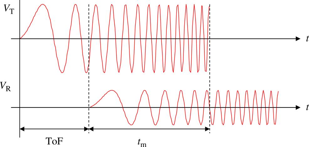
Assume the frequency varies linearly with time, starting from a lowest value fL, and increasing with a rate k (Hz/s): f(t)=fL+k·t. Due to the time delay of the reflected wave, its frequency in the same time frame is f(t)=fL+k·(t−τ). At any moment within the time period tm where the signals occur simultaneously, the frequency difference between the transmitted and the received wave equals:
(9.20)
with τ the ToF. The distance to the reflecting surface follows from
(9.21)
Apparently this distance is directly proportional to the frequency difference and unambiguous over a time tm as illustrated in Fig. 9.12. The CWFM method combines the advantages of the first two methods: The transmitted signal is continuous (favorable for the S/N ratio, uninterrupted distance information) and the range is larger (determined by the frequency sweep). Disadvantages over the burst method are the more complex interfacing and the fact that only wide-band transducers can be applied since the frequency varies. Further since transmission is essentially continuous, two transducers are required for simultaneous transmitting and receiving.
Important parameters of a CWFM system are the sweep length, the start and stop frequencies, and the sweep rate k (in Hz/s). The sweep length should correspond to the largest distance to be measured, to guarantee sufficient time overlap between the transmitted and reflected waves. The start and stop frequencies are set by the characteristics of the transducer. Electrostatic transducers for low-cost applications have a rather limited frequency range, typically from 50 to 100 kHz, so just one octave (a factor of 2). Usually the size of an electrostatic transducer in this frequency range is larger than that of a piezoelectric transducer. This may be a disadvantage from the viewpoint of construction; however, as has been shown in Section 9.2.1, the half angle is much smaller, contributing to a better S/N ratio of the echo signal.
According to Eq. (9.21) the distance measurement requires the determination of the frequency difference between transmitted and received signals. Usually this is done by some correlation procedure, performed in the digital signal domain (see, i.e., Refs. [33,34]). This has the advantage of noise reduction (depending on the type of filtering), but the disadvantage of the need to digitize and sample both signals. However, the procedure is essentially based on the multiplication of both signals, followed by some filtering. The basic goniometric relation of Eq. (9.22) is used:
(9.22)
So multiplying two sine waves results in a signal containing sum and difference frequencies. Now let the transmitted FM signal be:
(9.23)
The reflected wave signal delayed over a time τ becomes:
(9.24)
The product of these two signals contains components with sum and difference frequencies. Since we are only interested in the frequency difference, the much higher frequencies are filtered out and what remains is of the form
(9.25)
 (9.25)
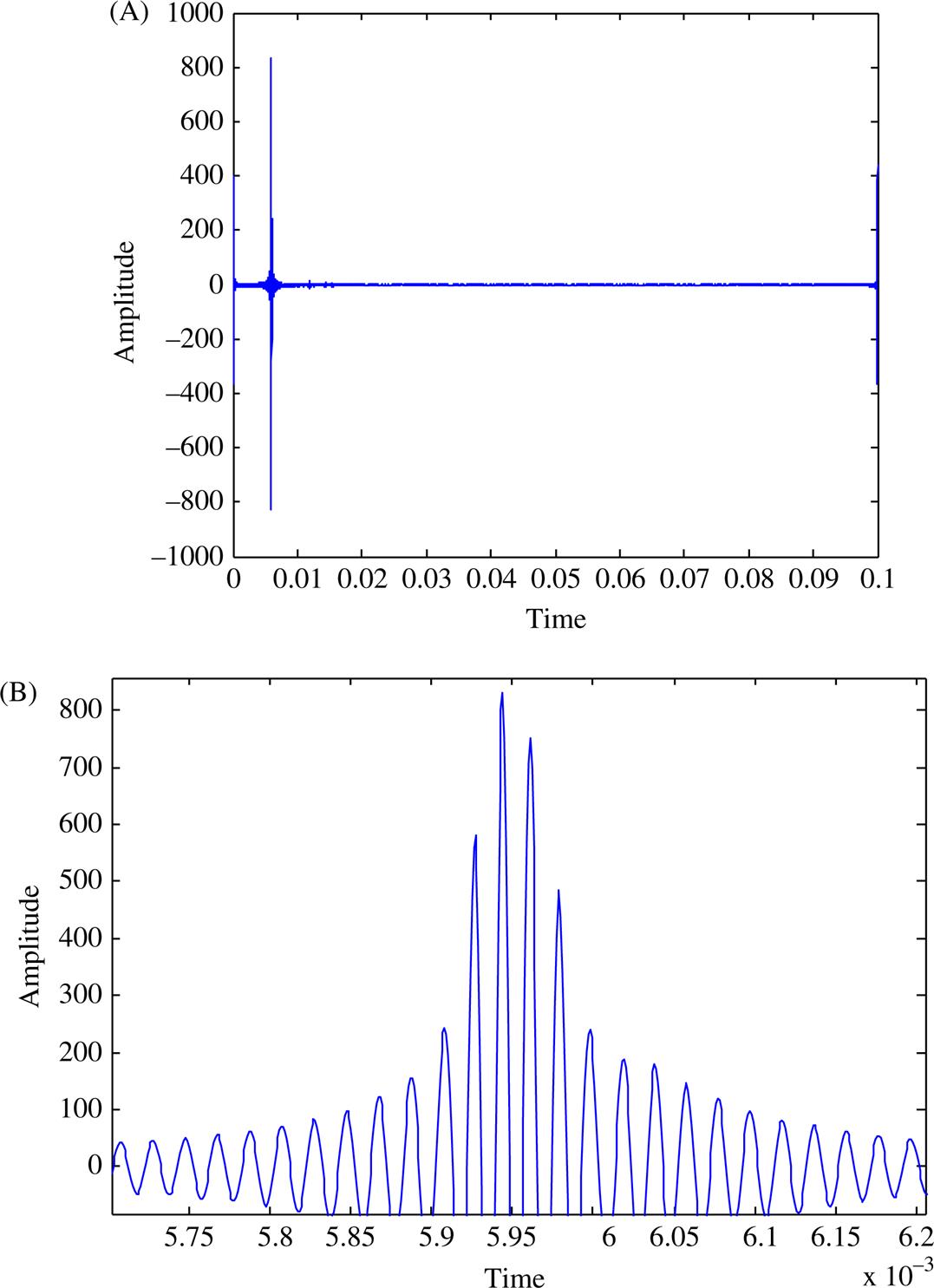
This clearly shows that multiplication produces a signal containing the frequency difference. Obviously for an accurate determination of this frequency all other components due to the multiplication procedure as well as noise should be sufficiently suppressed by some method of filtering. A treatment of the various signal processing algorithms goes beyond the scope of this book. To get an impression of a possible output Fig. 9.13 presents the result of a ToF measurement based on CWFM with matched filtering, applied to the signal reflected from a flat surface at 1 m distance. The horizontal time scale corresponds to the delay time (or ToF). In Fig. 9.13A the full scale is just the cycle period (100 ms). At around 0.006 s a pronounced maximum is noticeable. In the zoomed version Fig. 9.13B this peak appears to occur at 5.95 ms, corresponding with a distance of 1.02 m (at a measured sound frequency of 343 m/s). This figure also shows that the resolution of the measurement is limited: due to noise it may happen that an adjacent peak has a larger amplitude, introducing an error in the ToF determination.
Whether burst mode or continuous mode should be applied strongly depends on the requirements and the application. In general the burst method is simple to realize but is discontinuous and noise sensitive. CWFM is less sensitive to noise but requires more complicated interfacing and signal processing [35,36]. Generally speaking the CWFM method outperforms the burst method in terms of range and noise immunity.
9.3.4 Other signal types
Common to all methods considered thus far is the accurate determination of the time delay of an acoustic wave. Apart from the three signals discussed, many other signal types could be used to measure the ToF. Assuming the total transfer from transmitter, acoustic medium and receiver is linear (which is the case in the majority of the applications considered here), any signal containing some time-discriminating parameter will do.
A short, needle-like pulse is one of these. However, the bandwidth of most transducers is too small for handling such signals, and moreover, for air applications the energy content is too low. Gaussian noise is another one. The autocorrelation of wide-band Gaussian noise is a narrow peak. When such a noise signal is applied to the transmitter, cross correlation with the received signal results in a narrow peak in the correlogram at a position equal to the ToF. Limitations of this method are mainly of a practical nature: the noise signal and the transducers are always band limited, while sampling, AD conversion, and the finite measurement time further limit the resolution and accuracy of the digitally processed signals.
Another approach is phase shift or frequency shift keying. The signal is a (sinusoidal) carrier modulated in phase or frequency by a binary-coded signal. Such signals are now widely used in telecommunication, but may also play a role in acoustic distance sensing. An example of an application of binary phase shift keying signals for acoustic distance measurement in air is given in Ref. [37].
9.4 Applications
The versatility of ultrasound sensing is widely recognized. Ultrasonic sensors are extensively used in the processing industry for a variety of parameters [38], but they can also be found in numerous other fields, such as transportation, medical diagnostics, material research, and so on. The focus of this chapter is on the application in mechatronics, for a variety of tasks, with distance as the basic measurement quantity. These tasks comprise movement control in production machines, obstacle avoidance in traffic, navigation of automated guided vehicles (AGVs), object recognition and inspection, and many more. Acoustic sensors are cheap, small, and easily mountable on or in a mechatronic construction. When moderate distance accuracy is required, the interfacing can be kept simple. All measurements are based on the ToF principle as outlined in the previous section. We review two main tasks: Navigation and inspection.
9.4.1 Navigation
9.4.1.1 General
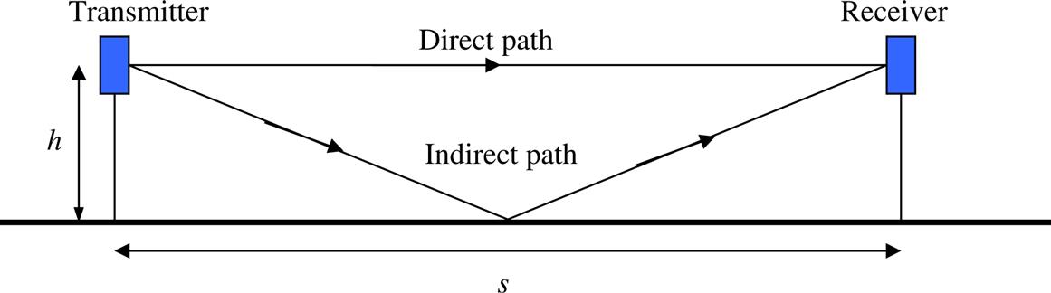
Acoustic transducers are suitable for short-range navigation in structured or unstructured (unknown) environments. Application examples are mobile robots (e.g., path finding and collision avoidance), aids for visually impaired people, and localization of tools in a work space. Common to these applications is the extraction of 2D or 3D information about the relative position of persons and objects in a mostly unconditioned environment. The easiest task is collision avoidance, because the demands with respect to accuracy and speed are not severe. Depending on further requirements various options can be considered. A simple anticollision system for robots and other vehicles like cars and wheelchairs consists of a number of fixed transducers at the front or around the circumference of the vehicle. The method works well if the reflecting obstacle has sufficiently large dimensions (at least a few wavelengths of the sound signal) and is oriented perpendicularly to the main axis of the transducer and in the absence of multiple echoes.
When the reflecting surface is not perpendicular to the main axis of the transducer, an error is introduced (compare Fig. 9.9). As a consequence the range data obtained by an acoustic scanning system show the typical behavior as seen in the sonar maps in Fig. 9.14. Simulations of such errors are extensively discussed in literature [39].

In Fig. 9.14 the transmitter/receiver combination rotates over an angle α with respect to the surface normal, and the dots represent measurement points. Range data are only available when the echo signal exceeds the detection threshold. Assume that this happens only when the reflected beam falls within the half angle of the receiver (an arbitrary choice because the threshold level may be adjusted to any other value). In Fig. 9.14A range data lie on an arc spanning twice the half angle of the transducers. In case of a rather sharp edge as in Fig. 9.14B, the acoustic wave reflects away from the receiver, so no echo is received. In practice, however, such an edge gives an echo regardless, but only over a small scanning angle. In Fig. 9.14C the received echo of a wave transmitted into the direction of the edge is mainly the result of multiple reflections in that edge. As can be seen in Figs. 9.14B and C even a small rotation angle results in a rather large distance error. Obviously in these cases the detectivity depends greatly on the angle between the two surfaces.
Erroneous distance data can be avoided by narrowing down the beam angle of the transmitter and receiver, but this is at the expense of lost data points (dead angles).
Similar to the optical system the ultrasonic counterpart may be disturbed too by spurious signals from other sources or unwanted reflections. In a natural, unconditioned environment, spurious echoes are unavoidable.
When such echoes interfere with the main echo, phase information is easily corrupted, even when the amplitude of the unwanted echo is small. Systems using ToF determination by thresholding detection are rather insensitive to this phenomenon: Time windowing may suppress most of the unwanted echoes since the direct wave arrives first in time. In systems based on envelope detection such spurious echoes may introduce large ToF errors, as shown in Fig. 9.15. More advanced detection methods are required to overcome this problem [40,41].

The performance of acoustic echo location in air is further determined by the power and frequency of the emitted pulse. Typical working distances of low-cost anticollision systems range from tens of centimeters (limited by the dead zone) to a few meters.
Ultrasonic distance sensors are also widely used in consumer products, from the sometimes inaccurately named parking “radar” systems to distance measurement in photo cameras. Polaroid introduced the ultrasonic ranging sensor (P6500) in 1981 (http://polaroid.com/history) for its autofocus camera model, shown in Fig. 9.16. This particular sensor also found its use in robotics, as obstacle sensor in early mobile rovers or walking machines.
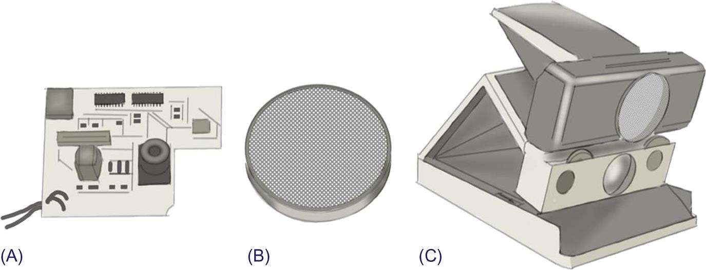
The system in this camera used electrostatic transducers, which were rather complicate to interface to other systems (Section 9.2.2). Current designs of ultrasonic range finders have a similar range (up to several meters) but use piezotransducers which can be used at lower voltages. Integrated modules are available, either with a single transducer which needs to switch from transmission to receiving mode after transmitting a “burst” of sonic pulses or versions with two transducers; usually a matched transmitter–receiver pair.
9.4.1.2 Navigation for mobile robots
Ultrasonic rangefinding is an excellent technique for the exploration of an unknown environment, to find the position and orientation of a robot in a known environment and to navigate. There is an overwhelming number of papers on this topic, dealing with many kinds of system concepts and signal processing algorithms. Most of these concepts are applied for autonomous navigation without beacons. Navigation with acoustic beacons is a low-cost alternative for the optical beacon systems discussed in Chapter 7, Optical Sensors.
Important design consideration is that the whole environment (e.g., walls, obstacles and persons) fall in the field-of-view of the sensing system, so not only in the direction of movement but also sideways and backwards. Three approaches can be followed:
An example of the first approach is presented in Ref. [42], in which an angular accuracy of less than 1 degree using eight transducers is reported. An obvious advantage of a (mechanical) scanning system is the need for just one or a very few pair of transducers; the scanning, however, is slow. A further point of consideration is the directivity of the transducers: A high lateral resolution over a wide viewing angle (possibly up to 360 degrees) requires a larger number of transducers with high directionality; the same coverage can be achieved with fewer transducers but with reduced lateral resolution.
Due to the relatively large wavelength of ultrasonic sound in air, the lateral resolution is rather low. This complicates the detection of small-sized objects or to distinguish between closely spaced objects, which is important in applications like a floor-cleaning robot [43] or navigation systems for blind persons. Enhancement of the lateral resolution without greatly increasing the number of transducers or their directivity (which is limited anyway) can be achieved by more advanced signal processing, e.g., potential fields [44] (applied for wheel chair navigation) and a one-transmitter three-receiver configuration [45]. A well-known method is the convolution of the echo signals with the transmitted signals. This may potentially improve both the lateral and the radial resolutions of an echo-location system, as is shown in Fig. 9.17. This figure shows the outcome of an experiment with two coffee cups placed on a flat table; the rotating piezoelectric transducers are positioned in the origin. Due to the wide beam angle the two cups are seen as one object. By deconvolution (using the known pulse response of the transducers) they can be distinguished separately.

Another approach to handling multiple objects is presented in Ref. [46] where the information from the echo amplitude is also used to construct a sonar map.
Navigation of vehicles or robots can be accomplished by a totally different approach based on beacons. Such beacons can be transmitting, receiving, or passive. In case of receiving beacons the robot generates continuous or intermittent signals all around. From the signals received by the beacons the distance to the robot can be derived. With known beacon positions the position of the robot is easily derived (Fig. 9.18). In general a minimum of three beacons is required to determine unambiguously the robot’s 2D position in an open space.
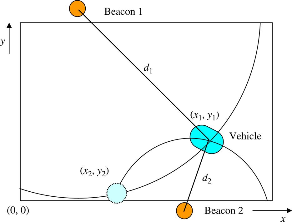
The reverse also works: Transmitting beacons send out unique signals, picked up by a robot equipped with an omnidirectional receiver. From these signals an on-board robot computer determines its distance from the beacons and subsequently its 2D position. A combination of these two possibilities is applied in an accurate docking system for AGVs [47].
In a system with passive beacons the robot transmits and receives signals, reflected by the beacons. Concerning the beacons this is by far the most simple and flexible concept. They need no power supply and the only requirements are an accurately known position and sufficient reflectivity for the signals. A disadvantage is a higher demand on environmental conditions, to prevent spurious reflections.
9.4.1.3 Navigation tool for visually impaired persons
This particular application of ultrasound sensing has attracted increased interest over the last few decades. Researchers have developed various concepts based on ultrasound ranging, like electronic dogs, canes, belts, and hats, all comprising some acoustic ranging device [48–51]. Fixing the acoustic transducers somewhere on the body leaves the hands free; attaching the transducers on a person’s head allows exploration of the environment in a more natural way. The detection area of the transducers may also be adapted to the immediate need and situation [52].
For this application it is important to not only avoid obstacles, but also to characterize or identify objects in the person’s immediate environment. The FMCW method yields such information [53], but the number of classes is very limited.
The technical problems to overcome are similar to those encountered in robot navigation. A particular challenge is the demand for safe operation outdoors, or in a noisy, heavily unstructured, and unconditioned environment. A completely different approach to many of these systems is still in the experimental phase, but there is noticeable progress in performance. With the availability of cheap cameras (webcams) nowadays, navigation tools are being developed based on a combination of acoustic ranging and vision.
9.4.1.4 Localization of tools
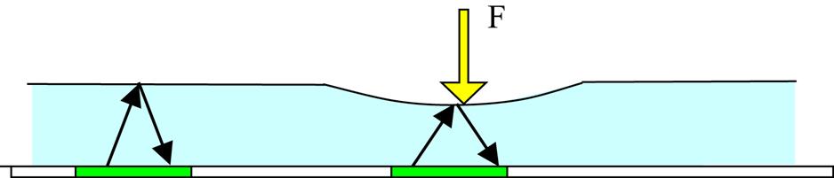
When a moving object is provided with a sound source, its position and orientation can be determined by using a set of acoustic sensors located at fixed points in the working space, similar to the beacon concept discussed earlier. In this way, the (3D) position of the end-effector [54] of a robot or its orientation with respect to a reference plane [55] can be determined. A different approach, presented in Ref. [56], combines a 2D vision system (fixed above the manipulator) and an acoustic distance sensor, together enabling 3D positioning of the robot gripper with respect to the object. Another example is the localization of surgical tools [57], where a position accuracy of 40 μm is reported.
In all these applications, special care should be taken to secondary echoes from floor, walls, and other objects in the surrounding tools. They may cause phase errors and a shift in the envelope top of the received signal (see Fig. 9.15), of which the consequences have already been discussed. Fig. 9.19 illustrates a situation where reflections via the ground floor may cause interference errors.
Assume the sound frequency is 40 kHz, corresponding with a wavelength of 8 mm. When the path difference equals an odd number of half a wavelength (i.e., at 4 mm, 12 mm, and so on) destructive interference of the received signals occurs. On the other hand at multiples of a full wavelength path difference (i.e., 8 mm, 16 mm, and so on) constructive interference takes place. The differences are rather common in many practical situations. Since the amplitudes of the sound waves differ, interference is only partial, to an extent that depends on the angles with respect to the acoustical axis of the transducers and on the reflectivity of the surfaces. Serious ToF errors occur at smaller distances and in the vicinity of many reflecting objects.
9.4.2 Inspection
9.4.2.1 General
Compared to 3D vision the technique of acoustic ranging suffers from a much lower spatial resolution. Conversely an acoustic ToF measurement system can be implemented in a cost-effective way, provides depth information and is less susceptible to environmental conditions (except for temperature variations, see Section 9.1). This explains why ultrasound ranging techniques for object recognition have been studied since the first decade of industrial robotics; see, e.g., Ref. [58], presenting a system based on ToF in the z-direction and spatial scanning using an x–y table, and [59] (2D angular scanning). We discuss three particular approaches: Acoustic imaging in air as an alternative for imaging by vision, NDT and inspection by touch using ultrasound-based tactile sensors. A series of examples for process monitoring using ultrasound concludes this chapter.
9.4.2.2 Acoustic imaging
The goal of any imaging system is the acquisition of an electronic picture from which information about an object’s size and shape can be inferred, preferably including as many details as feasible. In an adverse environment in particular, acoustic imaging could be a good alternative for the well-known optical imaging with cameras. Since the spatial resolution of an acoustic distance measurement is relatively low, some method of scanning is required to obtain detailed shape information. The performance of an ultrasonic recognition system is limited by the nature of sound waves, the properties of the transducers, the quality of the scanning system, the number of transducers, and the signal processing. In general the acquired image data are sparse and not accurate, which complicates recognition. However, in many applications the resolution requirements are not severe.
Scanning can be performed in various ways. Either the objects move relative to fixed transducers, or the transducers are moving relative to a fixed object. In a robotics environment a robot can perform the scanning, thereby making use of the many d.o.f.s of the manipulator to perform 3D scanning all around the object [60]. The encoders in the joints provide the orientation of the scanning range finder. A height map is obtained by Cartesian scanning in a plane above the scene. Sideways scanning enables the reconstruction of the circumference of an object, from the position and orientation of the flat or curved sides [61–63]. Several processing algorithms have been proposed to reconstruct the object shape from the obtained data or to classify the objects, including digital filtering, holographic algorithms, and artificial neural networks [64–66].
In all these examples mechanical scanning is used. The recognition of objects from a fixed sensory system has been studied as well. Usually such systems comprise an array of transducers with relatively large spacing [67]. For an accurate characterization of large objects (3–10 m), a set of transmitters/receivers is positioned around the object in such a way that together they cover the whole area of interest. An accuracy analysis of such an approach can be found in Ref. [68]. One of the difficulties in such a system is to distinguish between multiple objects and between various shapes returning similar echo patterns. These problems are solved using a set of transmitters and/or receivers at known relative positions and proper signal processing.
For the classification of objects with known shape, the “signature method” can be applied [62,69,70]. In this approach no attempt is made to reconstruct the object shape from the range data. Instead the system is taught to associate each object class with a characteristic echo pattern. A typical problem to be overcome in this approach is to obtain image data that are position and orientation invariant. On the other hand different but similarly shaped objects may result in echo patterns that are also similar. Correct classification on the basis of the echo patterns then requires special processing techniques, as described, e.g., in Ref. [71]. For objects with clearly distinguishable echo patterns the method is quick, requires simple hardware and software and is cost-effective.
9.4.2.3 NDT and material properties
Sound waves reflect at the boundary of two materials with different acoustic impedances. This property allows the measurement of many geometrical parameters of an object, just by applying sound waves to the device under test and the analysis of the waves reflecting at existing boundaries. One of the applications is the detection and localization of defects (e.g., voids and flaws) in a solid, even when invisible at the outside. The detection of small defects requires waves with a correspondingly short wavelength and therefore a much higher frequency compared to applications in air, typically in the MHz range. To a certain extent the size and shape of defects can also be reconstructed from the echo pattern [72–74].
Another application area is the measurement of layer thickness; the acoustic technique is used in a wide spectrum of materials and products, ranging from (steel) plates [75] to layers of paint [76] and in a human tooth [77]. To achieve high accuracy advanced signal processing is required. As an example in Ref. [78] the thickness of a multilayered structure is measured with an accuracy less than 10 μm for the individual layers. With the touch sensor in Ref. [79], thickness and hardness are simultaneously measured by a combination of acoustic and capacitive sensing elements.
Where acoustic damping (see Section 9.1.3) is an unwelcome effect in most of the applications discussed so far, this property of sound can be used to identify, monitor, or determine particular properties of a material. It is a suitable method in cases where the relation between the unknown parameter and the damping constant is known, e.g., by an acknowledged model or by calibration. Again there are numerous examples to illustrate this technique. We give just one example: The measurement of bubbles in liquids [80]. Both the acoustic attenuation and the speed of sound are related to the volume ratio of the two phases. By measuring these parameters over a relevant frequency range, various liquid properties can be deduced or evaluated.
9.4.2.4 Production and process control
The next list is an illustration of the versatility of acoustic sensing as an aid in production and process control; the references given are only examples of the many scientific papers published on these topics over the last decades.
- • Vibration measurements (example: a vibrating cantilever, phase detection of an 80 kHz sound wave [81])
- • Seam tracking (example: short-range scanning with a MHz piezoelectric transducer with focusing surface [82])
- • Respiratory air flow (example: two CW waves from piezoelectric transducers, with slightly different frequencies [83])
- • Liquid level (example: in bottles, 220 kHz piezoelectric sensors, burst mode [84]; as an acoustic resonator [85])
- • Go/no-go decision on product quality (example: quality of foundry pieces; signature imaging and Artificial Neural Network (ANN) for identification [86]; defect detection in food can production line: same method, according to Fig. 1.4 [87])
- • Air bubbles volume in liquids (example: PVDF-based T/R system, burst mode at 2 MHz bursts [88])
- • Speed of sound measurement (example: acoustic resonance determination by a piezoelectric (ceramic) tube [89])
- • Automotive (example: active suspension control; ToF measurement of backside vehicle to ground, 40 kHz burst mode [90])
- • Body movement (example: head movement relative to a computer screen, using three transmitters on the head and three receivers near the screen [91])
- • Paper roughness (using the roughness-dependent reflection of ultrasound [92])
The number of applications where a ToF measurement can be used is almost unlimited, and the reader is referred to the vast amount of literature in books and journals on NDT for further examples and inspiration.
9.4.2.5 Tactile sensors
Tactile sensors are used either to extract shape information on the basis of touch or to provide haptic feedback to the operator of manipulators as for instance in surgery. A tactile sensor consists of a matrix of force-sensitive elements (taxels). The tactile force is transformed into a deformation of some elastic material, and this deformation is measured using some displacement measuring method. So a tactile sensor provides a pressure or deformation image of the object with which it is brought into contact. General design aspects of tactile sensors have been considered in Section 4.4.3 on resistive sensors, where the aspect of taxel selection was also discussed. In this section we focus on ultrasonic measurement of the deformation, which is mostly based on the ToF method. Evidently it requires an acoustic transmitter–receiver combination for each taxel and a means for selecting the individual taxels. Usually a piezoelectric material is used, allowing small dimensions of the taxels. PVDF has several advantages over ceramic materials: it is available in sheets, it is a flexible material (matching well with the shape of robot grippers and fingers) and it has a favorable acoustic impedance (Section 9.1.4).
One of the first sound-based tactile matrix sensors is described in Ref. [93]. Fig. 9.20 shows the basic structure. The elastic top layer of this 3×4 matrix is responsible for the force-deformation transfer. Clearly the echo time changes proportionally to the compression of the layer and hence the applied force. The spatial resolution is about 1 mm. The ToF, determined by the layer thickness and the acoustic velocity, amounts to about 5 μs.
A similar construction, but with the elastic layer in between transmitter and receiver, is proposed in Ref. [94]. A completely different approach is described in Ref. [95]. The basic assumption here is that touch is accompanied by ultrasound. A quad PVDF sensor at the bottom of a sphere-shaped touch element enables the detection of this sound as well as the direction and hence the point of touch. The authors expect the sensor also be sensitive to slip. Indeed when an object is slipping this will generate vibrations, and hence sound; this information (as a binary sensor) can be used to control delicate gripping [96]. Another type of tactile sensor, presented in Ref. [97], is able to detect the friction coefficient, basically by measuring the resonance frequencies of an elastic cavity comprising a transmitter–receiver combination.
9.4.3 Interfacing acoustic sensors to embedded systems
The electrostatic and piezoelectric devices can act as transmitter as well as receiver for acoustic signals. Proper interfacing is required to realize these functions. The electronic circuits discussed in Appendix C can be used for this purpose. For embedded systems special modules have been designed to facilitate the interfacing.
The piezoelectric modules depicted in Fig. 9.21 contain the required amplification and filtering electronics for transmitting and receiving pulses. The resonance frequency of these piezotransducers is 40 kHz (Section 9.2.3). Usually the modules also contain a small microcontroller which is programmed to send out a “burst” of a predefined number of pulses, as well as controlling the moment the sensor switches from transmission to reception. In some cases, the microcontroller on the sensor module also processes the signals. This allows direct interfacing to a host microcontroller system by generating an analog voltage or a communication (bus) signal such as logic-level asynchronous serial communication or I2C.
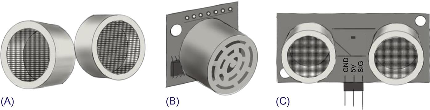
Most (relatively simple) modules contain a digital input (trigger) and output (signal). The host microcontroller system provides a pulse on the trigger input and measures the time it takes for the echoed burst to arrive at the output, thus effectively measuring the signal’s ToF t. The measured distance amounts l=½v·t, with v the speed of sound (Section 9.4.1). Sometimes the input and output pin on the module are combined to one pin. In that case the host controller starts by sending a pulse from a pin configured as output to the module, changes the pin to input and listens for the response. It is advisable to specify a time-out (or a window) when listening for responses, specified by the maximum range of the used sensor. Many libraries for interfacing ultrasonic range finders to microcontroller systems exist. Typical resolution of these sensors is in the order of millimeters.
9.4.4 Conclusion
This section on applications clearly demonstrates that the applicability of acoustic (ultrasound) sensors is almost unlimited. The major advantages of acoustic sensing over optical sensing are the lower sensitivity to dirt, smoke, and environmental light; the instantaneously obtained depth information (in ranging); and the ability to sense inside an object (in NDT). Significant disadvantages are the low resolution and the temperature sensitivity (due to the temperature dependence of sound speed). The latter drawback can easily be eliminated by an additional temperature compensation. For very high accuracy one should also consider the effect of humidity on the speed of sound, and possible air turbulence, introducing noise. When designing a mechatronic system it is worthwhile to make an extensive comparison between the two basic sensing concepts: Acoustic versus optical.