B.1 Generalized equations

In Chapter 2, Sensor fundamentals, a classification of quantities based on thermodynamics is presented. Here we review the basic equations extended with the magnetic domain.

The first law of thermodynamics is:

$\text{d}Q=\mathrm{\Theta }\text{d}\sigma$ (B.1)

(B.1)

with Θ is the absolute temperature and dσ is the increase in entropy of the system. According to the second law of thermodynamics the energy content of an infinitely small volume of an elastic dielectric material changes by adding or extracting heat dQ (J) and by work dW (J) exerted upon it

$\text{d}U=\text{d}Q+\text{d}W\text{(J)}$ (B.2)

(B.2)

The work dW is the sum of the different energy forms involved (here thermal, mechanical, electrical, and magnetic energy), so

$\text{d}U=\mathrm{\Theta }\text{d}\sigma +F\text{d}x+V\text{d}Q+I\text{d}\mathrm{\Phi }\left(\mathrm{J}\right)$ (B.3)

(B.3)

When the heat is taken per unit of volume, this equation reads:

$\text{d}U=\mathrm{\Theta }\text{d}\sigma +T\text{d}S+E\text{d}D+H\text{d}B(\mathrm{J}/{\text{m}}^3)$ (B.4)

(B.4)

that is the change in internal energy when thermal, mechanical, electrical and magnetic energy is supplied to the system. Note that for entropy we have used the same symbol but the dimension is now J/Km³.

Apparently, in this equation only through-variables affect the system. If, on the other hand, only across-variables affect the energy state of the system, the equation for the energy change per unit volume is:

$\text{d}G=-\sigma \text{d}\mathrm{\Theta }-S\text{d}T-D\text{d}E-B\text{d}H(\mathrm{J}/{\text{m}}^3)$ (B.5)

(B.5)

where G is the Gibbs free energy of the system, which can be found from the free energy U by a Legendre transformation.

We can generalize Eq. (B.4) as

$\text{d}U=\sum _i{A}_i\text{d}{B}_i\left(\text{J}/{\text{m}}^3\right)$ (B.6)

(B.6)

where A_i and B_i are conjugated pairs of variables. Note that the terms intensive and extensive have lost their original meaning in these equations. From Eq. (B.6) it follows for the parameters A_i

$A_i=\frac{\partial U}{\partial B_i}$ (B.7)

(B.7)

On the other hand, the system configuration or the material itself couples the conjugate variables of each pair. For instance, in the mechanical domain, T and S are linked by Hooke’s law:

$T=c·\mathit{S}\text{or}S=s·T$ (B.8)

(B.8)

where c is the elasticity (or stiffness) and s the compliancy.

In general, the intensive variable A_i and the extensive variable B_i within one domain are linked according to

$A_i=c_i·B_i\text{or}{B}_i=s_i·A_i$ (B.9)

(B.9)

where c_i is a (generalized) elasticity and s_i is a (generalized) compliancy. These are the state equations of the system.

From Eqs. (B.3) and (B.4) it follows that the system energy depends on all (generalized) parameters:

$U=f\left(A_i,B_i\right),\mathit{i}=1\cdots n$ (B.10)

(B.10)

but since A_i and B_i are related by Eq. (B.9) we can also write:

$U=f\left(B_i\right),\mathit{i}=1\cdots n$ (B.11)

(B.11)

So for small variations in the parameters B_i the variation in energy (as given in Eq. (B.6)) becomes:

$\text{d}U=\frac{\partial U}{\partial B_1}\text{d}{B}_1+\cdots +\frac{\partial U}{\partial B_n}\text{d}{B}_n=\sum _i^n\frac{\partial U}{\partial B_i}\text{d}{B}_i=\sum _i^n{A}_i\text{d}{B}_i$ (B.12)

(B.12)

Equation (B.9) links parameters within one domain. However, variables in one domain are also linked to variables in another domain, resulting in cross effects, the basis for transducers. So

$A_i=f\left(B_j\right),\mathit{i},j=1\cdots n$ (B.13)

(B.13)

and consequently, assuming linearity (small variations only):

$\text{d}{A}_i=\frac{\partial A_i}{\partial B_1}\text{d}{B}_i+\cdots +\frac{\partial A_i}{\partial B_n}\text{d}{B}_n=g_{i1}\text{d}{B}_1+\cdots +g_{in}\text{d}{B}_n=\sum _{j=1}^n{g}_{\mathit{ij}}\text{d}{B}_j$ (B.14)

(B.14)

where g_ij represents material properties linking domains i and j. Inversely parameter B_j depends on all parameters A_i. So the relations between small variations in parameters A_i and B_j can be described by

$A_i=g_{\mathit{ij}}·B_j\text{or}{B}_j=g_{\mathit{ji}}·{\mathit{BA}}_i$ (B.15)

(B.15)

The co-efficients g_ij and g_ji are equal. This can be proven by combining Eqs. (B.14) and (B.7):

$\frac{\partial A_i}{\partial B_j}=g_{\mathit{ij}}=\frac{{\partial }^{2}U}{\partial B_j{\partial B}_i}=\frac{{\partial }^{2}U}{\partial B_i{\partial B}_j}=g_{\mathit{ji}}$ (B.16)

(B.16)

since the order of differentiation can be reversed.

B.2 Application to four domains

The starting point is Eq. (B.5) for the mechanical, electrical, magnetic and thermal domains, which is repeated here in this order:

$\text{d}G=-S\text{d}T-D\text{d}E-B\text{d}H-\sigma \text{d}\text{Θ}\left(\text{J}/{\text{m}}^3\right)$ (B.17)

(B.17)

The through variables can be written as

$\begin{array}{c}S\left(T,E,H,\mathrm{\Theta }\right)=-{\left(\frac{\partial G}{\partial T}\right)}_{E,H,\mathrm{\Theta }}\\ \mathrm{D}\left(T,E,H,\mathrm{\Theta }\right)=-{\left(\frac{\partial G}{\partial E}\right)}_{T,H,\mathrm{\Theta }}\\ B\left(T,E,H,\mathrm{\Theta }\right)=-{\left(\frac{\partial G}{\partial H}\right)}_{T,E,\mathrm{\Theta }}\\ \sigma \left(T,E,H,\mathrm{\Theta }\right)=-{\left(\frac{\partial G}{\partial }\right)}_{T,E,H}\end{array}$ (B.18)

(B.18)

Since we consider only small variations, the variables S, D, B, and Δσ are approximated by linear functions, so

$\left[\begin{array}{c}\text{d}S\left(T,E,H,\mathrm{\Theta }\right)\\ \text{d}D\left(T,E,H,\mathrm{\Theta }\right)\\ \text{d}B\left(T,E,H,\mathrm{\Theta }\right)\\ \text{d}\sigma \left(T,E,H,\mathrm{\Theta }\right)\end{array}\right]=\left[\begin{array}{cccc}{\left(\frac{\partial S}{\partial T}\right)}_{E,H,\mathrm{\Theta }}& {\left(\frac{\partial S}{\partial E}\right)}_{T,H,\mathrm{\Theta }}& {\left(\frac{\partial S}{\partial H}\right)}_{T,E,\mathrm{\Theta }}& {\left(\frac{\partial S}{\partial \mathrm{\Theta }}\right)}_{T,E,H}\\ {\left(\frac{\partial D}{\partial T}\right)}_{E,H,\mathrm{\Theta }}& {\left(\frac{\partial D}{\partial E}\right)}_{T,H,\mathrm{\Theta }}& {\left(\frac{\partial D}{\partial H}\right)}_{T,E,\mathrm{\Theta }}& {\left(\frac{\partial D}{\partial \mathrm{\Theta }}\right)}_{T,E,H}\\ {\left(\frac{\partial B}{\partial T}\right)}_{E,H,\mathrm{\Theta }}& {\left(\frac{\partial B}{\partial E}\right)}_{T,H,\mathrm{\Theta }}& {\left(\frac{\partial B}{\partial H}\right)}_{T,E,\mathrm{\Theta }}& {\left(\frac{\partial B}{\partial \mathrm{\Theta }}\right)}_{T,E,H}\\ {\left(\frac{\partial \sigma }{\partial T}\right)}_{E,H,\mathrm{\Theta }}& {\left(\frac{\partial \sigma }{\partial E}\right)}_{T,H,\mathrm{\Theta }}& {\left(\frac{\partial \sigma }{\partial H}\right)}_{T,E,\mathrm{\Theta }}& {\left(\frac{\partial \sigma }{\partial \mathrm{\Theta }}\right)}_{T,E,H}\end{array}\right]=\left[\begin{array}{c}\text{d}T\\ \text{d}E\\ \text{d}H\\ \text{d}\text{Θ}\end{array}\right]$ (B.19)

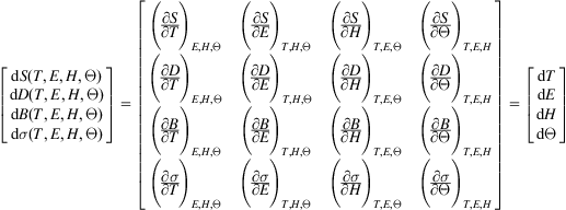(B.19)

Combining Eqs. (B.18) and (B.19) results in

$\left[\begin{array}{c}\text{d}S\\ \text{d}D\\ \text{d}B\\ \text{d}\sigma \end{array}\right]=\left[\begin{array}{cccc}{\left(\frac{{\partial }^{2}G}{\partial T^2}\right)}_{E,H,\mathrm{\Theta }}& {\left(\frac{{\partial }^{2}G}{\partial T\partial E}\right)}_{H,\mathrm{\Theta }}& {\left(\frac{{\partial }^{2}G}{\partial T\partial H}\right)}_{E,\mathrm{\Theta }}& {\left(\frac{{\partial }^{2}G}{\partial T\partial \mathrm{\Theta }}\right)}_{E,H}\\ {\left(\frac{{\partial }^{2}G}{\partial E\partial T}\right)}_{H,\mathrm{\Theta }}& {\left(\frac{{\partial }^{2}G}{\partial E^2}\right)}_{T,H,\mathrm{\Theta }}& {\left(\frac{{\partial }^{2}G}{\partial E\partial H}\right)}_{T,\mathrm{\Theta }}& {\left(\frac{{\partial }^{2}G}{\partial E\partial \mathrm{\Theta }}\right)}_{T,H}\\ {\left(\frac{{\partial }^{2}G}{\partial H\partial T}\right)}_{E,\mathrm{\Theta }}& {\left(\frac{{\partial }^{2}G}{\partial H\partial E}\right)}_{T,\mathrm{\Theta }}& {\left(\frac{{\partial }^{2}G}{\partial H^2}\right)}_{T,E,\mathrm{\Theta }}& {\left(\frac{{\partial }^{2}G}{\partial H\partial \mathrm{\Theta }}\right)}_{T,E}\\ {\left(\frac{{\partial }^{2}G}{\partial \mathrm{\Theta }\partial T}\right)}_{E,H}& {\left(\frac{{\partial }^{2}G}{\partial \mathrm{\Theta }\partial E}\right)}_{T,H}& {\left(\frac{{\partial }^{2}G}{\partial \mathrm{\Theta }\partial H}\right)}_{T,E}& {\left(\frac{{\partial }^{2}G}{\partial {\mathrm{\Theta }}^2}\right)}_{T,E,H}\end{array}\right]=\left[\begin{array}{c}\text{d}T\\ \text{d}E\\ \text{d}H\\ \text{d}\text{Θ}\end{array}\right]$ (B.20)

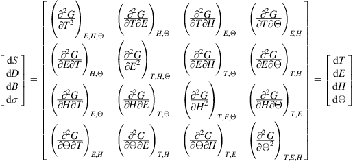(B.20)

The second-order derivatives in the diagonal represent properties in the respective domains: mechanical, electrical, magnetic and thermal. All other derivatives represent cross effects. These derivatives are pair-wise equal, since the order of differentiation is not relevant. The derivatives in Eq. (B.20) represent material properties; they have been given special symbols. The variables denoting constancy are put as superscripts, to make place for the subscripts denoting orientation.

$\left[\begin{array}{c}S\\ D\\ B\\ \sigma \end{array}\right]=\left[\begin{array}{cccc}{s}^{E,H,\mathrm{\Theta }}& d^{H,\mathrm{\Theta }}& {\lambda }^{E,\mathrm{\Theta }}& {\alpha }^{E,H}\\ d^{H,\mathrm{\Theta }}& {\epsilon }^{T,H,\mathrm{\Theta }}& m^{T,\mathrm{\Theta }}& p^{T,H}\\ {\lambda }^{E,\mathrm{\Theta }}& m^{T,\mathrm{\Theta }}& {\mu }^{T,E,\mathrm{\Theta }}& i^{T,E}\\ {\alpha }^{E,H}& p^{T,H}& i^{T,E}& \frac{\rho }{\mathrm{\Theta }}{c}^{T,E,H}\end{array}\right]·\left[\begin{array}{c}T\\ E\\ H\\ \Delta \mathrm{\Theta }\end{array}\right]$ (B.21)

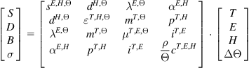(B.21)

The 16 associated effects are displayed in Table B.1.

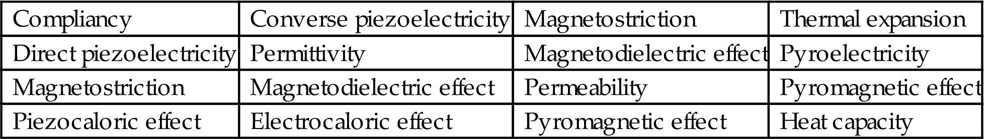
Some of these effects are mentioned in Fig. 2.6 (Chapter 6, Inductive and magnetic sensors), with the same or other names. The parameters ε, c_p and s correspond to those in Tables A.2, A.5 and A.8A of Appendix A. Table B.2 summarizes the parameters with symbols and units.

B.3 Heckmann diagrams

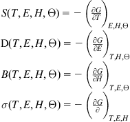
The material constants in the mechanical, electrical and thermal domains are defined by

$\begin{array}{c}\mathrm{mechanical:}\sigma =\frac{\rho }{c\text{θ}}·\text{θ}\\ {\mathrm{electrical:}S}_{\lambda }=s_{\lambda \mu }·T_{\mu }\text{or}{T}_{\mu }=c_{\lambda \mu }·S_{\lambda }\\ \mathrm{thermal}:D_i={\epsilon }_{\mathit{ij}}·E_j\mathrm{or}{E}_j={\beta }_{\mathit{ij}}·D_i\end{array}$ (B.22)

(B.22)

(compare Eqs. (A.5), (A.6) and (8.23)).

When extended with the mutual interactions between mechanical and electrical properties (piezoelectricity), four sets of equations can be defined, depending on the choice of the dependent and independent pairs of quantities. These equations are:

$\begin{array}{l}\{\begin{array}{c}{D}_i={\epsilon }_{ij}{E}_j+d_{i\mu }{T}_{\mu }\\ S_{\lambda }=d_{j\lambda }{E}_j+s_{\lambda \mu }{T}_{\mu }\end{array}\hfill \\ \{\begin{array}{c}{E}_j={\beta }_{ij}{D}_i-g_{j\mu }{T}_{\mu }\hfill \\ S_{\lambda }=g_{i\lambda }\cdot D_i+s_{\lambda \mu }{T}_{\mu }\end{array}\hfill \\ \{\begin{array}{c}{D}_i={\epsilon }_{ij}\cdot E_j+e_{i\lambda }{S}_{\lambda }\hfill \\ T_{\mu }=-e_{j\mu }{E}_j+c_{\lambda \mu }\cdot S_{\lambda }\end{array}\hfill \\ \{\begin{array}{c}{E}_j={\beta }_{ij}{D}_i-h_{j\lambda }{S}_{\lambda }\hfill \\ T_{\mu }=-h_{i\mu }{D}_i+c_{\lambda \mu }\cdot S_{\lambda }\end{array}\hfill \end{array}$ (B.23)

(B.23)

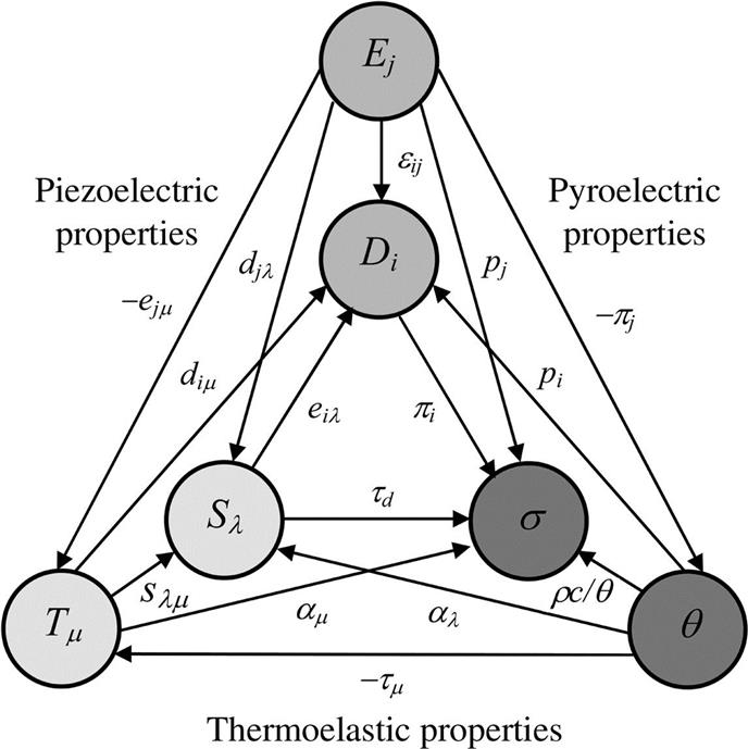
representing in total eight material properties: the reciprocal pairs s-c and ε-β, and four piezoelectric parameters (compare Table 8.1 in Chapter 8, Piezoelectric sensors). These relations are visualized in the Heckmann diagram for the electrical and mechanical domains (Fig. B.1). The circles represent the state variables, and the arrows represent the material properties.

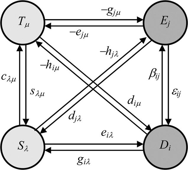
When the thermal domain is also included, sets of three equations can be defined. One of them is the set given in Chapter 2, Sensor fundamentals, by Eq. (2.10), yielding the most practical material properties. Fig. B.2 shows the Heckmann diagram for three domains, where the double arrows are left out for clarity.