
Sensor fundamentals
Abstract
In this chapter, we first introduce a notation system for the quantities used in this book and an unambiguous set of symbols for each quantity. Second, a formal description of relations between quantities, based on energy considerations, is presented from which particular physical effects are derived serving for specific groups of sensors that are discussed in later chapters. Various frameworks developed for a systematic description of sensors are briefly explained: they are based on measurand, application field, port models, conversion principles, and energy domain.
Keywords
Quantities; intensive and extensive variables; effort and flow variables; through- and across-variables; cross effects; sensor classification; port model; transducer model; sensor cube
A sensor performs the exchange of information (hence energy) from one domain to another and as such it operates at the interface between different physical domains. In this chapter, we first introduce a notation system for the quantities used in this book. To avoid confusion with notations, we define unambiguous symbols for each quantity. For example, in the electrical domain the symbol ε usually stands for dielectric constant, whereas it means strain in the mechanical domain. In this book, we use ε for dielectric constant only; strain is denoted by S. Several frameworks have been developed for a systematic description of sensors. Various approaches are presented in this chapter. Further, a formal description of relations between quantities, based on energy considerations, is introduced from which particular physical effects are derived serving for specific groups of sensors that are discussed in later chapters.
2.1 Physical quantities
2.1.1 Classification of quantities
Various attempts have been made to set up a consistent framework of quantities. Physical quantities can be divided into subgroups according to various criteria. This leads to subgroups with different characteristics.
Within one domain state and rate variables are related as follows:
(2.1)
- • With respect to energy:
a quantity that is associated with an energetic phenomenon: often called a variable (e.g., electric current and pressure);
a quantity that is not associated with energy or only with latent energy: often called a (material) property (e.g., length). Sometimes a property is also called a constant, but the value of most properties is not constant at all, so we will not use this term. - • With respect to dependency on mass or size:
a quantity which is independent of the dimensions or the amount of matter is called an intensive quantity (e.g., temperature is an intensive variable and resistivity is an intensive property);
a quantity which depends on the amount of mass or volume (its extension) is called an extensive quantity (e.g., charge is an extensive variable and resistance is an extensive property).Resistivity ρ (Ωm) is a pure material property, whereas the resistance R (Ω) depends on the material as well as the dimensions of the resistor body. In general, the relation between an intensive and extensive quantity within one domain is given by Ae=G·Ai, with Ae and Ai, general extensive and intensive quantities, and G, a geometrical parameter, representing for instance the dimension of a sensor. In most cases the value of a material property is orientation dependent. This dependency is expressed by subscripts added to the symbols (see Appendix A).
Extensive variables are state variables; their time derivatives are rate variables or flows. Intensive variables are identical to efforts. Flow and effort variables are discussed when conjugated pairs of variables are introduced. - • With respect to the end points of a lumped element:
To explain this classification, we first introduce the term lumped element. A lumped element symbolizes a particular property of a physical component. That property is thought to be concentrated in that element between its two end points or nodes. Exchange of energy or information occurs only through these terminals. In this sense we distinguish:
Through-variables are also called generalized I-variables; across-variables are called generalized V-variables. However, this is just a matter of viewpoint. It is perfectly justified to call them generalized forces and displacements. We will use these types of variables in Section 2.1.2 where relations between quantities are discussed.- • With respect to cause and effect:
Output variables are related to input variables according to the physics of the system. Input variables can bring a system into a particular state which is represented by its output variables. So output variables depend on the input variables:
independent variables are applied from an external source to the system;
dependent variables are responses of the system to the input variables.
Obviously, a variable can be dependent or independent, according to its function in the system. For instance, the resistance value of a resistor can be determined by applying a voltage across its terminals and measuring the current through the device or just the other way round. In the former case the voltage is the independent variable, and it is the dependent variable in the latter. The relation between independent and dependent variables is governed by physical effects, by material properties, or by a particular system layout. It either acts within one physical domain or crosses domain boundaries. Such relations are the fundamental operation of sensors. This is further discussed in Section 2.1.2. - • With respect to power conjugation:
Within a single energy domain, pairs of variables can be defined in such a way that their product is power. They are called power conjugated variables. The members of such a pair are called effort variable and flow variable. Table 2.1 lists these variables for various domains.
Note that the dimension of each product is power (W). The magnetic quantity “current” stems from the definition of magnetic field strength, where the number of ampere-turns (or magnetomotive force) determines the field strength (see Chapter 6). Its power conjugate variable “voltage” is actually the rate of change in magnetic flux, with unit Wb/s, but this is equal to the induction voltage. For practical reasons, heat flow (W) is often taken as the thermal flow variable rather than an entropy-related quantity which is not measurable in a straightforward way. The domain is therefore sometimes called pseudothermal (see last row of Table 2.1).
Table 2.2 summarizes various relations between rate, state, effort, and flow variables for the mechanical, electrical, magnetic, and thermal domains. - • With respect to energy conjugation:
Another way to define pairs of variables is based on the property that their product equals energy per unit volume (J/m3). Table 2.3 lists these pairs for the major domains.
The most fundamental categorization of quantities is based on thermodynamic laws. The description is in particular useful in the field of material research and optimization of sensor materials. Derived from the thermodynamic approach is the Bondgraph notation with a division of variables into effort and flow variables. This method is not only useful for the description of sensors but also has great significance in the design of all kind of technical systems, irrespective of the domain type.
Table 2.1
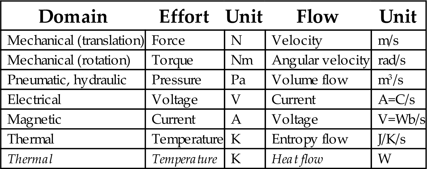
Table 2.2

Table 2.3

We repeat the list of pairs of the conjugate variables in Table 2.3, together with their symbols:
- • mechanical (translation): tension T (N/m2) and deformation S (–);
- • mechanical (rotation): shear tension τ (N/m2) and shear angle γ (–);
- • electrical: field strength E (V/m) and dielectric displacement D (C/m2);
- • magnetic: magnetic induction B (Wb/m2) and magnetic field strength H (A/m);
- • thermal: temperature Θ (K) and entropy σ (J/K m3).
Comparing these pairs with the groups from other categories given previously, we can make the following observations. The quantities E, D, B, H, T, and S are vector variables, whereas σ and Θ are scalars (therefore often denoted as Δσ and ΔΘ indicating the difference between two values). Further, in the above groups of quantities, T, E, and Θ are across-variables. On the other hand, S, D, and σ are through-variables. Finally, note that the dimension of the product of each domain pair is always J/m3 (energy per unit volume), whereas the product of the pairs effort and flow variables in Table 2.1 has the dimension power (W).
2.1.2 Relations between quantities
The energy content of an infinitely small volume of an elastic dielectric material changes by adding or extracting thermal energy and the work exerted upon it by electrical and mechanical forces. If only through-variables affect the energy content, the change can be written as follows:
(2.4)
where we disregard the magnetic domain (in Appendix B this domain is included).
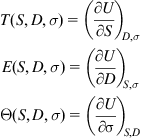
Obviously, the across-variables in this equation can be expressed as partial derivatives of the energy:
(2.5)
 (2.5)
(2.5)
Likewise, if only across-variables affect the energy content, the energy change is written as follows:
(2.6)
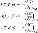
G is called the Gibbs potential (see Appendix B). The through-variables can be written as follows:
(2.7)
 (2.7)
(2.7)
From these equations we can derive the various material properties. We will extend these equations only for Eq. (2.7) because the resulting parameters are more in agreement with experimental conditions (constant temperature, electrical field strength, and stress), as denoted by the subscripts in Eqs. (2.5) and (2.7).
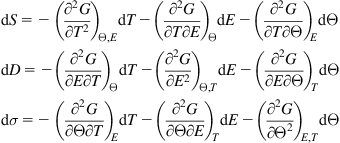
The variables S, D, and Δσ are approximated by linear functions, so:
(2.8)
 (2.8)
(2.8)
Combining Eqs. (2.6) and (2.7) results in:
(2.9)
 (2.9)
(2.9)
Now we have a set of equations connecting the (dependent) through-variables S, D, and σ with the (independent) across-variables T, E, and Θ. The system configuration (or the material) couples the conjugate variables of each pair. The second-order derivatives in the diagonal represent properties in the respective domains: mechanical, electrical, and thermal. For example, the top left second derivative in Eq. (2.9) represents the elasticity (or compliance) of the material (actually Hooke’s law). All other derivatives represent cross effects. Note that these derivatives are pair-wise equal since (assuming linear equations) the order of differentiation is not relevant:
So the derivatives in Eq. (2.9) represent material properties; they have been given special symbols. The variables denoting constancy are put as superscripts, to make place for the subscripts denoting orientation.
(2.10)
 (2.10)
For instance sE,Θ is the compliance at constant electric field E and constant temperature Θ. The nine associated effects are displayed in Table 2.4.
Table 2.4
| Elasticity | Converse piezoelectricity | Thermal expansion |
| Direct piezoelectricity | Permittivity | Pyroelectricity |
| Piezocaloric effect | Electrocaloric effect | Heat capacity |
Table 2.5 shows the associated material properties. The parameters for just a single domain (ε, cp, and s) correspond to those in Tables A.2, A.5, and A.8 of Appendix A. The other parameters denote “cross effects” and describe the conversion from one domain to another. The piezoelectric parameters p and d will be discussed in detail in the chapter on piezoelectric sensors.
Table 2.5
| Symbol | Property | Unit |
|---|---|---|
| s | Compliance | m2/N |
| d | Piezoelectric constant | m/V=C/N |
| α | Thermal expansion coefficient | K−1 |
| p | Pyroelectric constant | C/m2 per K |
| ε | Permittivity; dielectric constant | F/m |
| cp | (Specific) Heat capacity | J/kg per K |
Note that direct piezoelectricity and converse piezoelectricity have the same symbol (d) because the dimensions are equal (m/V and C/N). The same holds for the pair pyroelectricity and converse pyroelectricity as well as for thermal expansion and piezocaloric effect.
Eqs. (2.7) and (2.10) can be extended just by adding other couples of conjugate quantities, for instance from the chemical or the magnetic domain. Obviously, this introduces many other material parameters. With three couples we have nine parameters, as listed in Table 2.3. With four couples of intensive and extensive quantities we have 16 parameters, so seven more (for instance, the magnetocaloric effect, expressed as the partial derivative of entropy to magnetic field strength, see Appendix B). Further, Appendix B gives a visualization of these relations using Heckman diagrams.
2.2 Sensor classifications
A sensor (or input transducer) performs the conversion of information from the physical domain of the measurand to the electrical domain. Many authors have tried to build up a consistent classification scheme of sensors encompassing all sensor principles. Such a classification of the millions of available sensors would facilitate understanding of their operation and making proper choices, but a useful basis for a categorization is difficult to define. There are various possibilities:
These schemes will be briefly discussed in the next sections.
2.2.1 Classification based on measurand and application field
Many books on sensors follow a classification according to the measurand because the designer who is interested in a particular quantity to be measured can quickly find an overview of methods for that quantity. The more experienced designer may also consult books that deal with just one quantity (for instance temperature or liquid flow). Much information on sensors can also be found in books focusing on a specific application area, for instance (mobile) robots [1], industrial inspection [2], buildings [3], manufacturing [4], mechatronics [5], automotive, biomedical, and many more. However, an application field provides no restricted set of sensors since in each field many types of sensors could be applied.
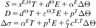
Fig. 2.1 presents a list of physical quantities (measurands) [6]. The list is certainly not exhaustive, but it shows the many possible measurands. For each of these quantities one or more measurement principles are available.
2.2.2 Classification based on port models
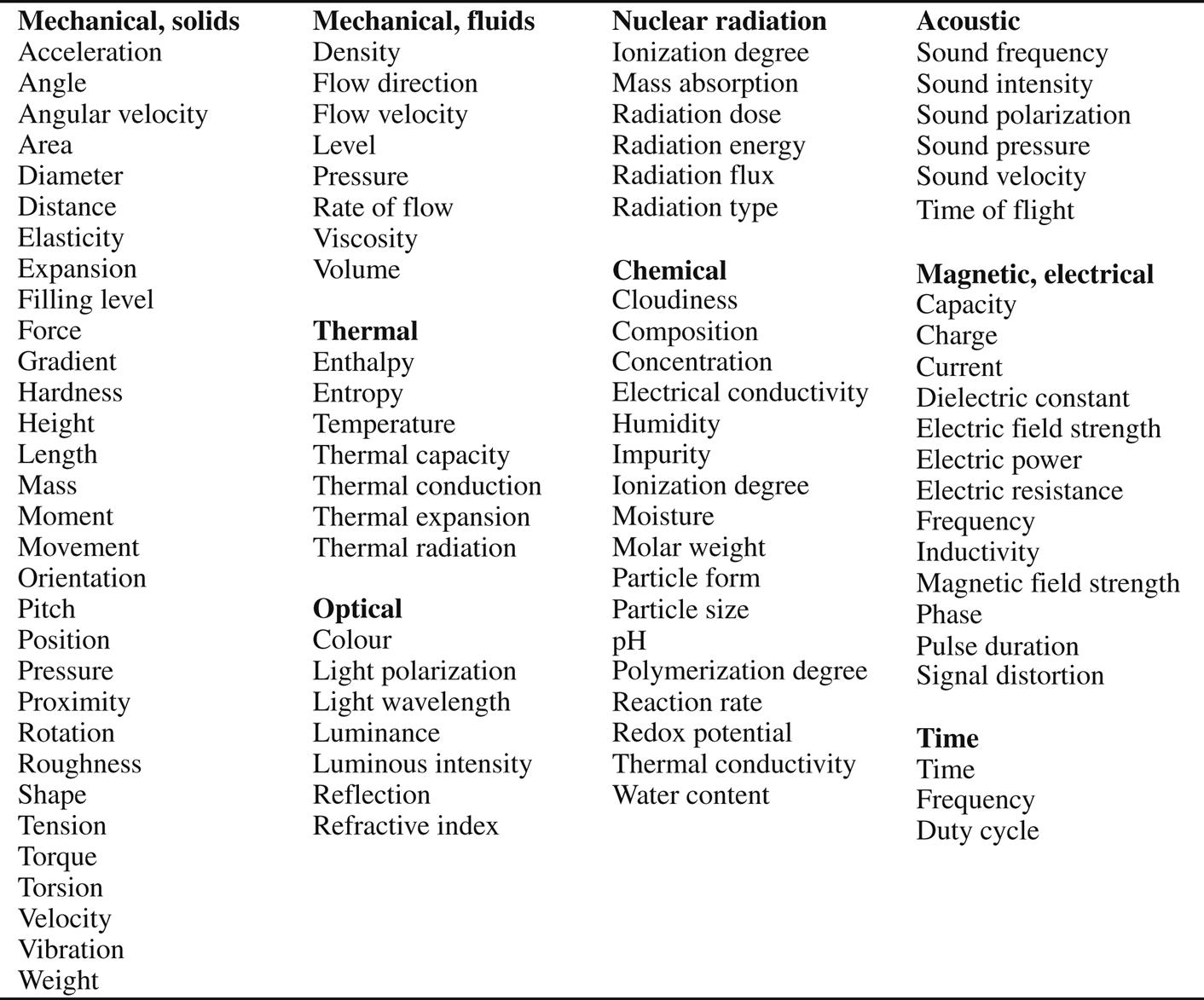
The distinguishing property in the classification based on port models is the need for auxiliary energy (Fig. 2.2). Sensors that need no auxiliary energy for their operation are called direct sensors or self-generating sensors. Sensors that need an additional energy source for their operation are called modulating sensors or interrogating sensors.
Direct sensors do not require additional energy for conversion. Since information transport cannot exist without energy transport, a direct sensor withdraws the output energy directly from the measurement object. As a consequence, loss of information about the original state of the object may occur. There even might be energy loss too—for instance, heat. An important advantage of a direct sensor is its freedom from offset: at zero input the output is essentially zero. Examples of direct sensors are the piezoelectric acceleration sensor and the thermocouple.
Modulating or interrogating sensors use an additional energy source that is modulated by the measurand; the sensor output energy mainly comes from this auxiliary source, and just a fraction of energy is withdrawn from the measurement object. The terms modulating and interrogating refer to the fact that the measurand affects a specific material property which in turn is interrogated by an auxiliary quantity. Most sensors belong to this group: all resistive, capacitive, and inductive sensors are based on a parameter change (e.g., resistance, capacitance, and inductance) caused by the measurand. Likewise, most displacement sensors are of the modulating type: displacement of an object modulates optical or acoustic properties (e.g., transmission, reflection, and interference), where light or sound is the interrogating quantity.
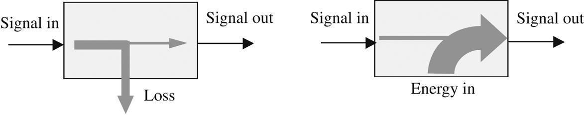
Energy (and thus information) enters or leaves the system through a pair of terminals making up a “port.” We distinguish input ports and output ports. A direct sensor can be described by a two-port model or four-terminal model (Fig. 2.3A).
The input port is connected to the measurand; the output port corresponds with the electrical connections of the sensor. Likewise, a modulating sensor can be conceived as a system with three ports: an input port, an output port, and a port through which the auxiliary energy is supplied (Fig. 2.3B). In these models the variables are indicated with across or effort variables ![]() and through or flow variables
and through or flow variables ![]() , respectively. The subscripts x, y, and z are chosen in accordance with the sensor cube, to be discussed in Section 2.2.4.
, respectively. The subscripts x, y, and z are chosen in accordance with the sensor cube, to be discussed in Section 2.2.4.
Direct sensors provide the information about the measurand as an output signal, an energetic quantity. Modulating sensors contain the information as the value of a material property, or a geometric quantity, not an energetic signal. The information enters the system through the input port, where the measurand affects specific material or geometric parameters. To extract the information from such a sensor, it has to be interrogated using an auxiliary signal. The information stored in the sensor is available latently, in the latent information parameters or LIPs [7]. These parameters are modulated by the input signal and interrogated by the auxiliary or interrogating input.
At zero input the LIPs of a modulating sensor have initial values, set by the material and the construction. Generally, the input has only a small effect on these parameters, resulting in relatively small deviations from the initial values. Note that direct sensors too have LIPs, set by materials and construction. They determine the sensitivity and other transfer properties of the sensor. So the input port of all sensors can be denoted as the LIP input port. As a consequence, any sensor can be described with the three-port model of Fig. 2.3B. Only the functions of the ports may differ, notably the LIP input port and the interrogating input port.
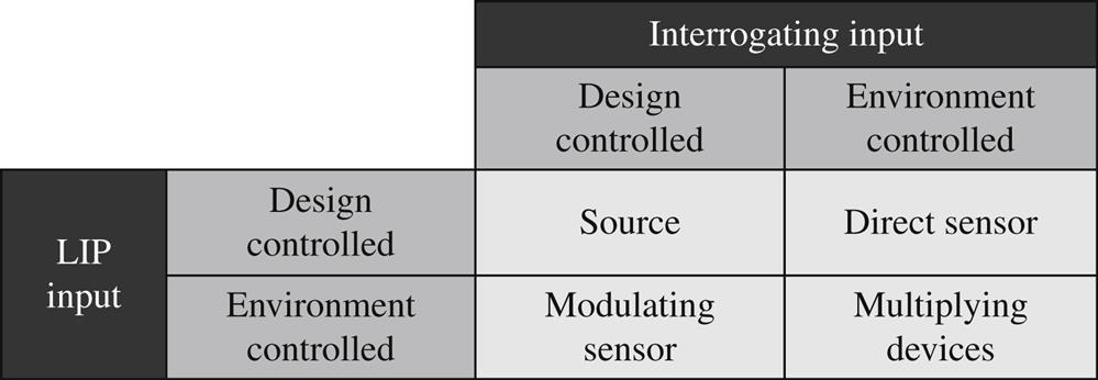
According to the “unified transducer model” as introduced in Ref. [7], an input port can be controlled either by design (it has a fixed value) or by the environment (the measurand or some unwanted input variable). So we have four different cases (Fig. 2.4). The characteristics of these four transducer types are briefly reviewed:
- • Design-controlled LIP input and design-controlled interrogating input.
All inputs are fixed. This type represents a signal or information source, for instance, a standard or a signal source with a constant or predetermined output. The output is totally determined by the construction and the materials that have been chosen. Any environmental effect on the output is (ideally) excluded. - • Design-controlled LIP input and environment-controlled interrogating input.
Since the latent information parameters are fixed by design, the output depends only on what is connected to the interrogating input. When this is the measurand, the transducer behaves as a direct sensor. Examples: - • Environment-controlled LIP input and design-controlled interrogating input.
The measurand affects particular material properties or geometric parameters. These changes are interrogated by a fixed or well-defined signal at the interrogating input. The transducer behaves as a modulating sensor. Examples:- • Strain gauge bridge: strain alters the resistance of the strain gauges; a bridge voltage converts this resistance change into an output voltage;
- • Linear variable differential transformer (LVDT): a displacement of an object connected to the moving core will change the transfer ratio of the differential transformer. An AC signal on the primary coil acts as interrogating quantity.
- • Hall sensor: the measurand is a magnetic induction field, which acts on moving charges imposed by a fixed (or known) current applied to the interrogating input.
- • Environment-controlled LIP input and environment-controlled interrogating input.
These are multiplying transducers: the output depends on the quantities at both inputs, often in a multiplicative relation. For instance, a Hall sensor could act as such, when the interrogating input is not a fixed current (by design) but a current that is related to just another measurand.
It is important to note that any practical transducer shows all four types of responses. A strain gauge (a modulating transducer) produces, when interrogated, an output voltage related to the strain-induced change in resistance. But the circuit can also generate spurious voltages caused by capacitively or magnetically induced signals. A thermocouple (a direct transducer) produces an output voltage proportional to the measurand at the interrogating input. If, however, the material parameters change due to (for instance) strain or nuclear radiation (inputs at the LIP port), the measurement is corrupted.
Since just one response is desired, other responses should be minimized by a proper design. The universal approach helps to identify such interfering sensitivities.
2.2.3 Classification based on conversion principles
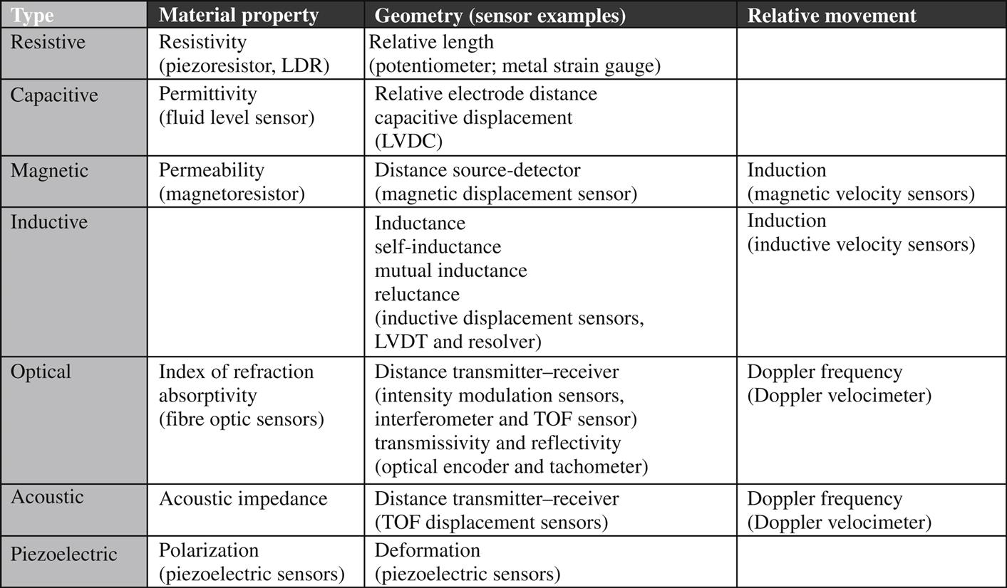
The classification according to conversion principles is often used for the reason that the sensor performance is mainly determined by the physics of the underlying principle of operation. However, a particular type of sensor might be suitable for a variety of physical quantities and in many different applications. For instance, a magnetic sensor of a particular type could be applied as displacement sensor, a velocity sensor, a tactile sensor, and so on. For all these applications the performance is limited by the physics of this magnetic sensor, but the limitations manifest in completely different ways. A closer look at the various conversion effects may lead to the observation that the electrical output of a sensor depends either on a material property or the geometry or a movement. Fig. 2.5 tabulates these three phenomena for various types of sensors.
2.2.4 Classification according to energy domain
A systematic representation of sensor effects based on energy domains involves a number of aspects. First, the energy domains have to be defined. Second, the energy domains should be allocated to both the sensor input and output. Finally, since many sensors are of the modulating type, the domain of the auxiliary quantity should also be considered. From a physical point of view, nine energy forms can be distinguished:
This classification is rather impractical for the description of sensors. Lion [8] has proposed only six domains and adopted the term signal domain. These six domains are: radiant, thermal, magnetic, mechanical, chemical, and electrical. The number of domains is a rather arbitrary choice, so for practical reasons we will continue with the system of six domains and call them energy domains.
Information contained in each of the six domains can be converted to any other domain. These conversions can be represented in a 6×6 matrix. Fig. 2.6 shows that matrix, including some of the conversion effects. An input transducer or sensor performs the conversion from a nonelectrical to the electrical domain (the shaded column), and an output transducer or actuator performs the conversion from the electrical to another domain (the shaded row). The cells on the diagonal of the matrix indicate effects within a single domain.

This two-dimensional representation can be extended to three dimensions, when the interrogating energy domain is included. This gives 216 energy triplets. To get a clear overview of all these possible combinations, they can be represented in a 3D Cartesian space, the “sensor cube” (Fig. 2.7). The three axes refer to the input energy domain, the output energy domain, and the interrogating input energy.
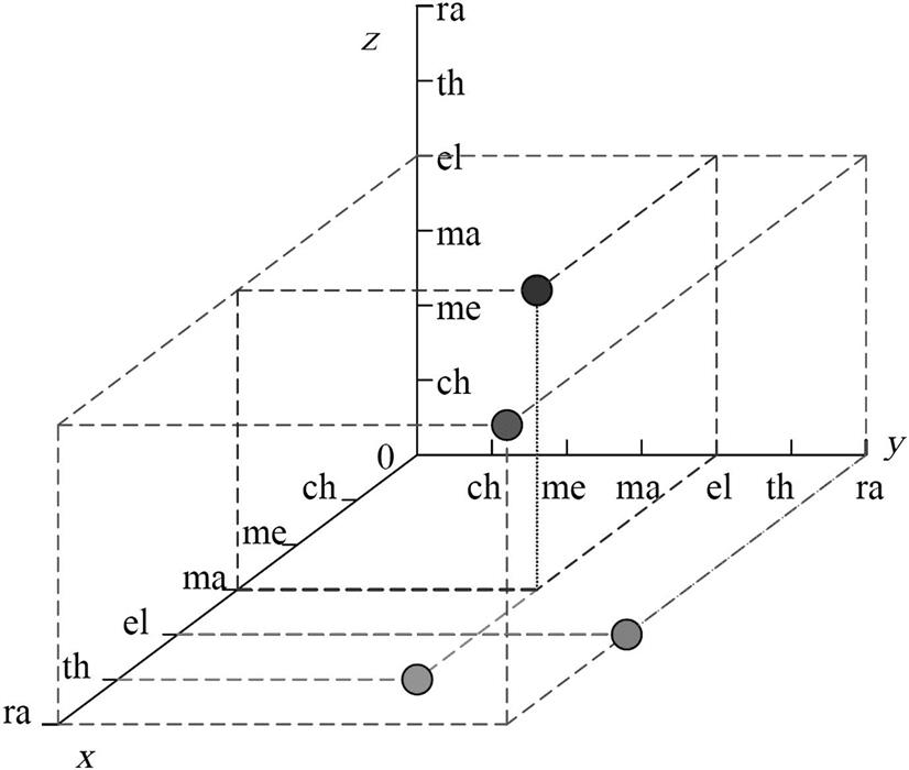
On each of the 216 elements of the 6×6×6 matrix a conversion effect is located. When restricting to electrical transducers, there are 5 direct input transducers, 5 direct output transducers, 25 modulating input transducers, and 25 modulating output transducers.
To facilitate notation, the transducers can be indicated by indices, like in crystallography, the so-called Miller indices: [x, y, z]. The x-index is the input domain, the y-index is the output domain, and the z-index is the domain of the interrogating quantity. With these three indices a transducer can be typified according to the energy domains involved. Some examples are as follows:
These transducers are also visualized in Fig. 2.7. The practical value of such a representation is rather limited. It may serve as the basis of a categorization for overviews or as a guide in the process of sensor selection.