Appendix A3
Propagation through the Atmosphere

When a laser beam is propagated through a substantial path length in the atmosphere, we experience a number of phenomena that affect the optical power carried by the beam and distort the wavefront. Usually, atmospheric effects are classified in two categories: (i) those associated with the non-ideal transparence of the atmosphere, notably absorption and scattering, called turbidity effects, and (ii) those coming from non-homogeneity of the index of refraction of the atmosphere, caused by thermal exchange and air mass motion, called turbulence effects.

A vast amount of literature is available on the subject (see, for example, Refs.[1-5]), and here we will report a few results to supply basic information useful for the evaluating performance of instruments treated in the text.

A3.1 Turbidity

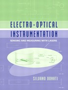
In general, a beam propagated through a medium on a path length L (Fig.A3-1) suffers a power loss, with respect to the initial value P₀ described by the Lambert-Beer law of attenuation:

(A3.1)

The quantities α and s are called the absorption and scattering coefficients of the medium, and their sum, a=α+s, is the (total) attenuation coefficient. Of course, a,α, and s are measured in m^-1 or cm^-1. Their inverse values represent the propagation length after which the initial power is decreased to 1/e=37% and are called the absorption, scattering, and attenuation lengths, respectively.

Figure A3-1 The attenuation of power propagated through a path length L follows the negative-exponential Lambert-Beer law

The quantity T= exp -(α+s)L is referred to as the transmittance.

In the atmosphere, absorption is due to constituent species (nitrogen, oxygen, carbon dioxide, etc.) and water vapor, while scattering is dominated by small-size (<1μm) particulate and eventually water droplets in the case of haze or fog.

The absorption contribution is fairly constant, whereas the scattering contribution strongly depends on weather conditions.

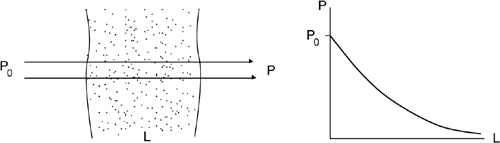
In Fig.A3-2 we report what is considered the most representative diagram [6] of atmospheric transmission T versus wavelength, measured at ground level on a normal, clear day on a path length of L=1800 m.

Figure A3-2 Standard atmospheric transmission (%) for a propagation on an L=1800 m length path at ground level

As we can see from Fig.A3-2, the atmosphere has a few transmission windows of reasonable transparency, useful for operating laser instrumentation on medium distances (say, 100 to 1000 m).

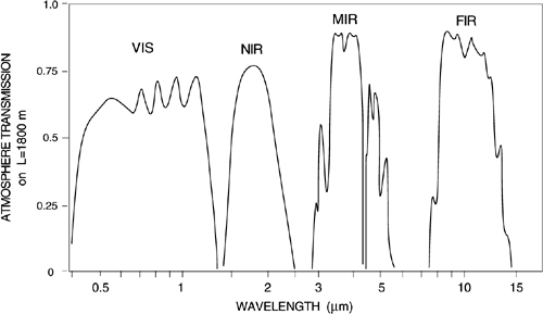
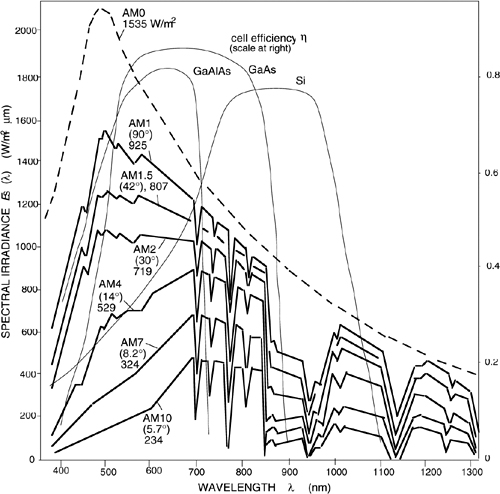
Another diagram useful for evaluating atmospheric transmission on larger distances (tens of km) is shown in Fig.A3-3. The diagram is the plot of solar spectral irradiance received at ground level on a clear day at different elevation angles θ of the sun on the horizon. The quantity AM=(cosθ)^-1 is the air mass number, and represents the equivalent number of atmospheres crossed by the rays at elevation θ. The curve with AM0 in Fig.A3-3 is the irradiance outside the atmosphere. The ratios of the values read on the curves at different AM# and at AM0 are the transmissions of the atmosphere for different elevations or air masses.

Figure A3-3 Spectral solar irradiance (W/m²μm) received at ground level for several elevation angles or air masses AM

In addition to the VIS (visible) window, we find the three well-known IR (infrared) windows of the:

- near-infrared (or NIR, λ=1.5-2.3 μm),

- middle-infrared (or MIR, λ=3-5 μm), and

- far-infrared (or FIR, λ=8-14 μm).

Beyond the FIR window, no other window is found up to millimeter waves. For a very dry atmosphere (RH<5%), there is actually a modest window at λ=330±10μm with a peak transmission T=5% (L=300 m), but T rapidly decreases with increasing relative humidity RH, going down to T<0.1% at RH=70%.

In the UV, the atmospheric transmission gradually decreases at shorter wavelengths until we reach VUV (vacuum-ultra-violet), requiring vacuum for propagation because of an intolerable loss, even for path that is a few centimeters in length.

In the visible range, the attenuation coefficient of a standard atmosphere has been computed from constituents as the sum a_st =α_oz+s_R+s_a of the following: ozone contribution α_oz(important for λ<290 nm), Rayleigh scattering s_R (important for λ<400 nm), and aerosol scattering s_a, giving a value a=0.18 km^-1 at λ-=500 nm.

The term s_a is dominant for λ>400 nm and gives the trend for total attenuation, a good approximation for λ= 0.5-5μm except for the narrow molecular absorption lines α_mol that must be added to the background value.

Data shown in Fig.A3-2 represent the transmission of the standard atmosphere and include the s_R and s_a terms. In addition to that, a much larger term, s_par, comes from scatterers extraneous to the clear atmosphere, such as particulate matter and small droplets.

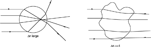
Scatterers are small-size particles that can be schematized as spheres randomly distributed in space, with a certain radius r_p and an index of refraction n_p. The radius is found to range from sub-μm size to over hundreds of μm, and the index of refraction is always well in excess of n_air=1 (e.g., n_p =1.33 for water droplets), the index of the surrounding medium.

Small size and large index of refraction difference is the peculiarity of turbidity. Conversely, turbulence is the regime where scatterers are large in size (mm to m) and their index of refraction difference is very minute (10^-6 to 10^-3) and may also fluctuate spatially and temporally.

Considering a small particle with a substantial Δn, the outgoing ray will largely deviate in angle on refraction inside and outside the particle (Fig.A3-4), whereas the deviation (or beam wandering) is very little if Δn is small. Also, as a large angular deviation brings the outgoing ray out of the beam, a scattered ray is equivalent to a lost ray, and thus scattering does contribute to attenuation. By contrast, the small deviation introduced by turbulence can be recovered by increasing the acceptance area of the detector and does not contribute to attenuation, at least in principle.

But, with turbulence, we will additionally have a random spatial mixing of contributions inside the beam, an effect called scintillation, which destroys spatial coherence.

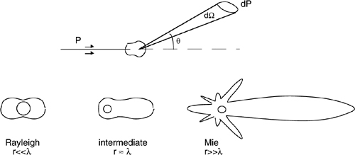
The quantity used to describe the angular scattering process is the scattering function, f(θ)dΩ=dP(θ)/4πP. It is defined as the relative power per unit solid angle Ω that we collect at the angle θ with respect to the θ=0 incidence (Fig.A3-4), 4π being a normalization factor.

Figure A3-4 Ray tracing through scatterers with a large Δn (turbidity, left) and a small Δn (turbulence, right) reveals the difference in angle deviation

Regarding the shape of the scattering function f(θ), the critical parameter is the ratio r/λ, and we can distinguish between two limit cases:

(i) for small particles, i.e., r<<λ, we are in the so-called Rayleigh scattering regime [3] and the function f(θ) is nearly isotropic. This means that we collect nearly as much power in the forward (θ≈0) as in the backward direction (θ≈π), the minimum being found at the right angle (θ≈π/2).

(ii) for very large particles, or r>>λ, we are in the Mie regime [3] and the scattering function is strongly peaked in the forward direction, and an appreciable contribution in the backward direction is left (Fig.A3-5).

Another important parameter to describe the scattering process is the cross-section A_sc of the scatterer, intended as the effective area subtended to incoming rays.

Figure A3-5 Top: definition of the scattering function f(θ). Bottom: the scattering function f(θ) in the Rayleigh and Mie regimes.

Like the scattering function f(θ), this quantity is calculated by an electromagnetic field analysis [3] of the scattering process. From the analysis, it is found that:

(A3.2)

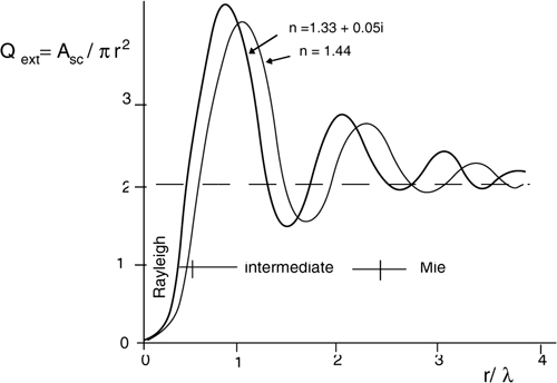
The factor Q_ext is called the extinction efficiency and is plotted in Fig.A3-6 versus the normalized radius r/λ. In the Rayleigh regime for small particles, the extinction efficiency Q_ext varies as (r/λ)^-4. The particles are seen from the electromagnetic radiation as if they were much smaller than their actual physical size. In the Mie regime for large particles, Q_ext=const ≈2 and particles are seen as twice as large as their actual radius. This apparently odd result is correct, because the diffraction contribution is found to be exactly equal to the physical obstruction produced by the particle.

Now we can sum up the effects of scattering. If we have a medium containing a concentration of c (cm^-3) particles per unit volume, each with an effective area A_sc, then the power remaining in the beam after propagation on a path length L will be:

(A3.3)

In addition, the power scattered in the far field at an angle θ..θ+Δθ from the incidence is P_sc= P₀ [1- exp-cA_scL] f(θ) 2πθΔθ.

Figure A3-6 The extinction efficiency versus the normalized radius r/λ. In the Mie region (r>>λ), Q_ext tends asymptotically to a constant (≈2), whereas in the Rayleigh region (r<<λ), Q_ext and the attenuation coefficient vary as (r/λ)^-4. There is also a minor dependence on Q_ext by the index of refraction of the droplet.

A quantity of importance, related to the attenuation coefficient, is the visibility range. Conventionally, the visibility range for vision through the atmosphere and other scattering media is taken as the value L_vis at which scene contrast is reduced to 2% of the initial value. This definition is related to the visual acuity of the eye, which can resolve a ≈2% contrast in good viewing condition [7]. As the contrast reduction is the same as the useful non-attenuated power, using Eq.A3.1 we find the visibility range as:

(A3.4)

Typical values of attenuation a, in km^-1 are the following:

0.18 for a clear atmosphere at sea level, (L_vis=22 km),

0.5-1 for a light haze (L_vis=7.8-3.9 km),

2-5 for thick haze (L_vis=1.9-0.78 km),

50-200 for a medium fog (L_vis=78-20 m),

300 for a thick fog (L_vis=13 m),

0.02-0.1 for an exceptionally clear atmosphere, with Rayleigh diffusion limit, seldom reached, of s_R=0.012 (L_vis=326 km).

Looking at the dependence of Q_ext from r/λ in Fig.A3-6, we can see that visibility in fog and haze can be improved by moving the wavelength of operation to the infrared.

Figure A3-7 The ratio L_a10/L_a0.7 of attenuation lengths at 10 μm (FIR) and at 0.7 μm (visible) versus the attenuation length in the visible L_a0.7 (from Ref. [8])

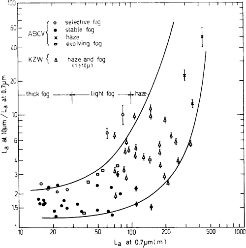
With a smaller r/λ, we may go from the Mie regime with Q_ext≈2 to the Rayleigh regime with Q_ext and attenuation proportional to (r/λ)^-4. In Fig.A3-7, we report experimental results on the FIR-to-visible ratio of attenuation length L_a10/L_a0.7, as measured by several researchers [8].

Other things being equal, this ratio is the expected visibility improvement. The ratio depends on L_a0.7, because the average radius of a particle changes with the type of turbidity, being small (r≈0.5μm) in hazes and fairly large (r≈0.5-10μm) in fogs.

In common conditions, the ratio L_a10/L_a0.7 may range from ≈1.5 for L_a0.7=20m (L_vis= 78m) to ≈5 for L_a0.7=150m (L_vis= 600m), up to perhaps ≈10 for L_a0.7=100m (L_vis= 390m). These values are very attractive in several applications, including navigation aids in automotive, avionics, and military systems.

Unfortunately, the improvement is the smallest at the shortest visibility range, where it would be the most desirable: in very thick fog, it may be down to about unity. In addition, the actual visibility improvement is appreciably less than is expected from the L_a10/L_a0.7 ratio. The reason is that the scene appearance changes appreciably from the visible to the FIR regions [16].

In the visible, the scene contrast is dominated by the surface diffusion coefficient, whereas in the FIR, it is determined by temperature differences [7]. Thus, an infrared scene has details correlated to the visible image, but with significant deviations introducing a task of identification to the observer, whereas detection and recognition [7,16] are easier.

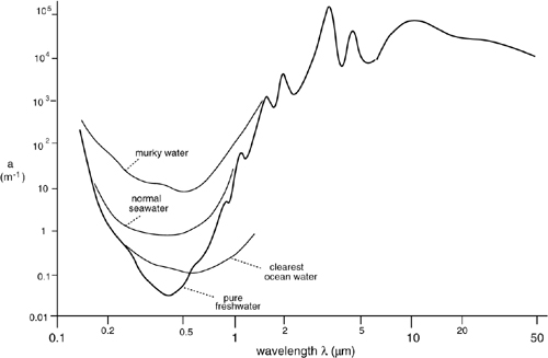
Figure A3-8 Typical dependence of attenuation vs. wavelength in water

In detection, improvements of visibility up to a factor 50 have been actually observed [9] on 10-km ranges with FIR imaging. For identification tasks, however, we should take account a difficulty factor [7]. This can be roughly estimated to decrease by a factor 2-3 the actual improvement with respect to the attenuation ratio L_a10/L_a0.7 [9].

Another natural medium of importance for electro-optical instrumentation is water.

As shown in Fig.A3-8, there is just one window in water, centered at 450 nm (blue-green), where the attenuation coefficient reaches the ultimate value of a=0.025 m^-1 for distilled water (L_vis=156 m). In very clear deep ocean waters, attenuation may reach, at λ=440 to 510 nm, a=0.05-0.1 m^-1(L_vis= 78-39 m, near Madeira island) [10], but usually it is a≈1 m^-1 and up to a≈10 m^-1 depending on particulate. In the maximum transparency window, the relative weight of diffusion s and absorption in attenuation a=s+α are 0.6 and 0.4, respectively, whereas outside (Fig.A3-8), absorption is dominant (α>>s).

A3.2 Turbulence

Propagation over a substantial distance (say, >10 m) in the atmosphere is affected by turbulence. Thermal exchanges with the ground and the sun’s heating are responsible for a daily temperature excursion producing convection and vortex in the air.

Because of the associated density fluctuations, the local index of refraction Δn has a small randomness superposed on the average value, and the propagated beam suffers a small angular deviation (Fig.A3-4).

If Δn were constant across the beam, there would be just a deflection, or a random wandering of the beam around the unperturbed direction. But, most frequently, the Δn scale of correlation is smaller than the size of the propagated beam after a substantial distance, and different portions of the beam are deflected differently.

As the result, the wavefront is distorted and the spatial distribution deviates from the Gaussian emitted from the laser, with dark and bright spots known as scintillation (Fig.A3-9).

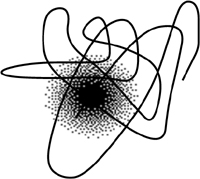
For such a distribution, the coherence factor μ_sp (Sect.4.5.3) of superposition at the detector is decreased. Also, when the wandering deviation is about the same as the spot size (Fig. A3-10), in addition to intensity fading, we face a serious speckle phase error (Sect.4.4.7).

The study of atmospheric turbulence is segmented into three steps: (i) assessing the statistical properties of Δn fluctuations, (ii) translating them into the statistics of the propagated optical field, and (iii) describing the consequent effect on the detected signal.

The details of the theoretical development are very complex, and here we will report just a few basic results, derived under a number of assumptions. An excellent review of turbulence is provided in the work of Hufnagel [11] and by other authors [12-14].

From the engineering point of view, nearly all the quantities of interest are related to C_n²∞Δn², called the structure constant, and associated with the correlation function defined as D_n(ρ)=[n₁(0)-n₂(ρ)]², where ρ is the distance between two points P₁ and P₂.

Tatarski [15] has found that D_n(ρ)= C_n²(ρ)^2/3, so the quantity C_n² is measured in m^-2/3.

Fig.A3-9 Scintillation of a 20 mW, w₀=1 mm He-Ne beam propagated through air at H=5m height from ground. Top: the beam spatial distributions (not to same scale) as they appear at L=0 (left), 40 m (center), and 200 m (right); exposure is 0.1-s. Bright spots change their position randomly in the beam cross-sections with a typical 0.1 to 1-s time scale. Bottom: profiles of intensity along a diameter exhibit an increasing number of spikes with L.

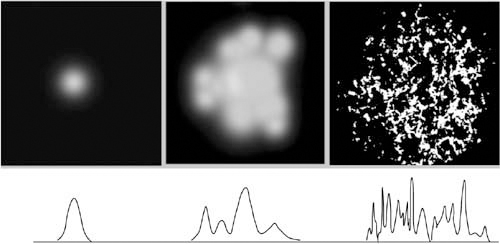
Fig.A3-10 Wandering of the propagated beam for an He-Ne laser (as in Fig.A3-8). The centroid of the beam cross-section (dotted circle) moves randomly in time around the average line-of-sight position.

The constant C_n² is easily connected to the temperature variance C_T²∞ ΔT² by the error propagation rule C_n²= (dn/dT)²C_T². The temperature coefficient is |dn/dT|≈1 ppm at sea level [see Eq.4.27] and decreases exponentially with height as |dn/dT|≈ exp–(H_(km)/12.6) [11].

According to the model of Kolmogorov [15], the kinetic energy of vortex is dissipated by friction on an inertial sub-range scale, spanning from a few mm to a few m. In this range, temperature fluctuations have a correlation D_T(ρ)= C_T²(ρ)^2/3, and Δn fluctuations have D_n(ρ)= C_n²(ρ)2/3, provided that l₀<ρ<L₀, where l₀ (≈mm) and L₀ (≈m) are called the inner and outer scales of turbulence.

Experimentally, the constant C_n² can range from ≈10^-15 to ≈10^-13 m^-2/3 for weak to strong turbulence, respectively, at sea level. The lowest values are found in the early morning and at dusk, in the absence of wind. With height, C_n² varies as H^-2/3 (low H or high wind) or H^-4/3 (high H or still air), with a break point at H≈1-10m.

To assess the effect of C_n² on the propagating optical beam, following Rytov [11,15], we can represent the electric field E= E exp[i(kr-ωt)+χ(r,t)+iφ(r,t)] as composed of an average part E with the usual propagation term exp i(kr-ωt), and of a random exponential attenuation χ(r,t) and phase disturbance iφ(r,t), both fluctuating and due to turbulence.

From the Rytov analysis, it is found that these random variables have zero mean values, χ=0, φ=0, and a normal distribution. Thus, the distribution of the attenuation exp χ is log-normal.

In the simple case of a horizontal path propagation (C_n²≈const) of a plane wave on a σ_χ² of the log-normal attenuation χ has been calculated [11] as σ_χ²=0.131·C_n² k^7/6L^11/6, with k=2π/λ being the wave number. For a spherical wave, the numerical factor is 0.546. Experimentally, the predicted values nicely match the measurements for σ_χ²<0.3, while for larger values a saturation is found at about σ_χ²≈0.5, which is typical for L≈ 300m or larger.

Correspondingly, the variance σ_E² of amplitude fluctuations is σ_E²=E²[(exp4σ_χ²)-1] and the variance of the intensity is I=E² is σ_I²=4I²(expσ_χ²-1).

About the phase variance σ_φ² Ishimaru [12] has reported that it is equal to σ_χ² or twice as much in the two cases and i.e., in the case of a turbulence scale of correlation l_c much smaller or much larger than the Fresnel-zone size , respectively. Conservatively, we may take σ_φ² ≈ C_n² k^7/6L^11/6 and find the maximum distance L at which the turbulence effect is negligible by equating σ_χ² to the value of accuracy required in our experiment. For example, letting σ_φ²=0.01(rad²), at λ=1μm we get L=47 m for a weak tur (C_n²=10^-15), but just L=3.8 m for a strong turbulence (C_n² =10^-13).

Beam wandering can be characterized by a radius ρ_w, defined as the rms value of the beam centroid deviation off the expected position. An approximate expression for a colli-mated beam is [12]: ρ_w= w/(1 - 2.45 C_n²k^1/3L^11/6w^-5/3), where w is the unperturbed beam size at distance L, or explicitly w²=w₀²+(λ/πw₀)²L² for a Gaussian beam.

At a relatively short distance, the beam shape is substantially unchanged and its centroid wanders randomly by a rms deviation ρ_w; The wandering has a characteristic time τ_w (given by ≈w/v_w, v_w being the wind velocity), and σ_χ², σ_φ² are negligible. On a time-scale slower than wandering time, the apparent beam size is w_turb w_turb²=w²+ρ_w². At a large distance, where ρ_w>>w, the beam no longer wanders appreciably, appears widened to a size w_turb with scintillation effects now showing up, and σ_χ², σ_φ² are no longer small.

A quantity of interest to interferometer operation through a turbulent atmosphere is the transverse coherence length S_t of the propagated beam, which corresponds to the speckle transversal size discussed in Sect.4.4.7 and is roughly the size of the individual grains found in both the scintillation and beam wandering regimes.

For propagation on a length L, the transverse coherence length is given by an approximate relation [16] as: S_t=(0.5 k²C_n²L)^-3/5. For example, at λ=1μm and L=200 m, we get S_t=40 cm for a weak turbulence (C_n²=10^-15) and S_t=2.6 cm for a strong turbulence (C_n2 =10^-13).

All these statistical results describe the point-like detection of amplitude and phase of the propagated field. Now, we can consider the effect of detector size. When we increase the detector diameter from d_det<<S_t up to the coherence size S_t, the average signal increases and the relative variance improves, such as σ_I²/I² =4 (expσ_χ²-1) for the intensity. For d_det >S_t, we collect uncorrelated samples of the χ and φ random variables, and the relative variance of intensity weakly improves, only as the logarithm of the number of coherence areas, or ln(1+d_det/S_t), while the phase variance is substantially unchanged.

Finally, regarding the frequency distribution of fluctuations, the power spectrum S(f) is related to the variance σ² by the Wiener-Khintchin theorem as ∫_0-∞ S(f)df=σ². If the spectrum falls off at a corner frequency f_tur, we can assume S(f) =σ²/f_tur as a reasonable first-order approximation. The corner frequency f_tur for both amplitude and phase fluctuations depends on the wind transversal velocity v_t as f_tur=l_c/v_t, where l_c is the turbulence scale of correlation. Typical values of the frequency corner are in the range of f_tur≈10 to 200 Hz.

References

[1] W.L. Wolfe and G.J. Zissis (editors), “The Infrared Handbook”, Environmental Research Institute of Michigan: Ann Arbor, MI, 1988.

[2] V.I. Tatarski, “Propagation of Waves in Turbulent Medium”, McGraw-Hill: N.Y., 1961.

[3] H.C. Van de Hulst, “Light Scattering by Small Particles”, J. Wiley: New York, 1957.

[4] Burle Industries Inc. “Electro-Optics Handbook”, Burle vol.TP-135, Lancaster, PA, 1992.

[5] OSA Staff, “Optics Handbook”, Opt. Soc. of Am.: Washington DC, 1992, vol 1.

[6] H.A. Gebbie et al., “Atmospheric Transmission in the 1-14 micrometer Region”, Proceedings of the Royal Society, vol.A206 (1951), pp. 87-96.

[7] S. Donati, “Photodetectors”, Prentice Hall: Upper Saddle River, NY, 2000, App.A3.

[8] S. Donati, “Optoelectronic Techniques for Navigation Aids in Poor Weather”, Alta Frequenza, vol.43 (1974), pp.725-732.

[9] S. Donati, “Thermal Imaging Through Hazes and Fog: Experimental Results”, Alta Frequenza, vol.42 (1973), pp.101-105.

[10] S. Duntley, “Light in the Sea”, J. Opt. Soc. of Am., vol.53 (1963), pp. 214-221.

[11] R.E. Hafnagel, “Propagation through Atmospheric Turbulence”, in The Infrared Handbook, edited by W.L. Wolfe and G.J. Zissis, IRIA: Ann Arbor, MI, 1978.

[12] A. Ishimaru, “Wave Propagation in Scattering Media”, vol.1 and 2, Academic Press: New York, 1978.

[13] A. Ishimaru, “Wave Propagation in Turbulent Media”, Proc. IEEE, vol.79 (1991), pp.1359-1366.

[14] R.L. Fante, “Electromagnetic Beam Propagation in Turbulent Media”, Proc. IEEE, vol.68 (1980), pp.1424-1443.

[15] V.I. Tatarski, “Propagation of Waves in a Turbulent Medium”, McGraw Hill: New York, 1961.

[16] G.R. Osche and D.S. Young, “Imaging Laser Radar in NIR and FIR”, Proc. IEEE, vol.84 (1996), pp.103-125.