Chapter 4
Laser Interferometry

Interferometry is one of the most powerful tools in measurement science. It provides a very high sensitivity, unequalled by any other techniques, and is widespread in virtually every segment of engineering and physics. Interference of light was one of the phenomena marking the birth of optics and challenging the seventeenth-century scientists to explain the nature of light, notably Newton and Huygens [1]. In the nineteenth century, though a good understanding of interference was reached, interferometry had few notable applications because of the limited coherence length of the sources then available [1]. With the advent of lasers in the 1960s, the full capability of this powerful technique was finally unleashed. Many impressive sensors and measurement devices were developed: submicrometer displacement interferometers, laser Doppler velocimeters, and gyroscopes, just to name the big engineering achievements of the electro-optical science.

In this chapter, we adopt a bottom-up presentation, first describing the operation of the instrument with a minimum of basics. Then, we expand the coverage by considering the many facets of modern interferometry. Among these, we will treat optical configurations, fundamental limits of sensitivity and accuracy, different schemes of superposition, and all the topics of general relevance. Other chapters in this book will deal specifically with applications of interferometry to velocimetry, gyroscopes, and fiberoptic sensors.

As a primer, let us now briefly outline the basic paradigm of interferometry.

A suitable source, usually a laser, is used to direct an optical beam into the experiment or the physical ambient to be sensed (Fig.4-1).

Fig.4-1 The conceptual scheme of interferometry (top) and the signal out from the photodetector (bottom)

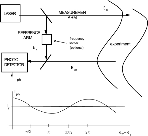
A fraction of the beam is kept in the instrument to be used as a reference. Upon returning back from the experiment, the measurement beam is superposed to the reference beam onto a photodetector.

If E_m and E_r are the optical fields of the two beams, the photogenerated current I_ph obtained as a signal out from the photodetector is:

(4.1)

where the fields E_m,r = E_m,r exp iφ_m,r have been represented as rotating vectors with amplitude E_m,r and phase φ_m,r, the bars (|..|) denote modulus, and σ is a conversion factor between current and squared field (or power). Developing Eq.4.1 yields:

(4.2)

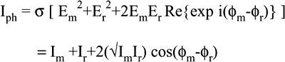
Here, I_m,r=σE_m,r² are the currents that the measurement and reference fields would provide individually, and the last term is the interference signal.

As we can see, the interference signal is proportional to the cosine of the optical phase shift φ_m-φ_r between measurement and reference beams. If we keep the reference beam fixed and unaffected by any disturbance (φ_r =const.), while the measurement beam carries the phase shift collected in the propagation, the signal from the photodetector is a quantity measuring the optical phase φ_m.

Usually, the beam propagates to a distant reflector and back, totaling a length 2s which amounts to a phase shift (2s/λ)2π=2ks, where λ is the wavelength, 2π is the number of radians per wavelength and k=2π/λ is the wave-number.

Apart from a constant term I_m+I_r, Eq.4.2 tells us that the interferometric signal is of the type cos 2ks (the cosine-signal), and its amplitude is proportional to , the geometric mean between reference and measurement powers.

This amplitude is times larger that of the signal I_m being detected alone. Thus, in the interferometer, there is a sort of internal gain, , of photodetection. This is a consequence of the beam superposition, resulting in a coherent scheme [3] of detection, a scheme further possessing the very welcome property of working at the quantum-noise limit of the received signal. Because of that, the sensitivity of the interferometer is very good, which is detailed later in this chapter.

4.1 Overview Of Interferometry Applications

Fig.4-2 presents a pictorial overview of the big tree of interferometry. Applications may be divided in the two branches of industrial/avionics and scientific measurements.

In the first, we find the well-established applications to the following:

– Mechanical metrology (positioning of tool machines, mechanical workshop calibrations, and measurements)

– Fluid anemometry (the so-called laser-Doppler velocimetry)

– Vibrometry (rotating machinery diagnostics and control)

In avionics, a very wide segment of application is covered by the gyroscope. This is an interferometer and senses the Sagnac phase shift induced by rotation. The gyroscope is the heart of inertial sensors like Inertial Navigation Units (INU), Heading Reference Systems (HRS), and attitude and spin control systems.

About scientific uses, a number of amazing examples of application have been successfully reported.

Fig.4-2 The tree of interferometry applications

Classifying them as in Fig.4-2 according to the distance or the baseline on which the measurement is performed, we find the following:

– Terrestrial tide monitoring (for geodesy)

– Satellite-to-subsatellite displacement pickup (to unveil mascons – mass concentrations useful to oil-field discovery)

– Long-distance vibrometry (for testing the structural integrity of towers, bridge and dams) and the metrology of length and derived quantity (gravimeter, thermal expansion of materials)

– Pickup of biological motility (respiration sounds and cells motility for fertility)

– Pickup of surface acoustic waves (study, design, and testing of SAW devices and AOM modulators).

Most recent on the long baseline end, we find the biggest interferometers ever built (or, near to completion), the Virgo and LIGO (Fig.1-11). These experiments are gravitational antennas based on an interferometer. They are aimed to detect very minute (10^-18m) bumps on a target mass acting as an antenna, coming from very remote (Megaparsec) sources of gravitational waves – giant-star collapses.

4.2 The Basic Laser Interferometers

The term laser interferometer is commonly used to indicate an electro-optical instrument capable of performing the measurement of displacement of a corner cube target, with a fraction-of-wavelength resolution and a 10^-6 accuracy or precision. The target is usually mounted on the carriage of a tool machine or the like, and the distance range covered by the measurement is up to the scale of meters.

Soon developed after the invention of the He-Ne laser in 1961, the laser interferometer has become a well-established instrument for measurements and especially calibration. The precision is exceptionally good because the scale factor is directly connected to the wavelength of the laser. This quantity can be easily stabilized to a relative accuracy better than Δλ/λ≈10^-8 in commercial, cheap He-Ne frequency-stabilized units (see Appendix A1).

Diode lasers are rapidly catching up in this application, but, to obtain at least Δλ/λ≈10^-6, we should have either a DBR laser diode, presently not yet available as standard products at visible wavelengths (610-680nm) where operation is preferable because of safety, or an external-grating stabilized diode, which is rather expensive.

Therefore, in the following, we refer to interferometers based only on the He-Ne laser.

In next sections, we describe the two main approaches considered the best for the development of practical laser interferometers: the dual beam and the two frequency.

Both approaches are used in commercial products, and give rise also to several variants in respect to frequency stabilization of the laser and/or electronic processing of the interferometric signals.

4.2.1 The Two-Beam Laser Interferometer

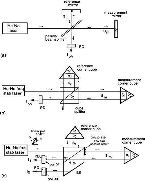
It may be instructive to follow the evolution of the Michelson interferometer, see Fig.4-3a, up to the modern two-beam laser interferometer of Fig.4-3c. As soon as the laser was available for use as the source in a Michelson interferometer, displacement measurements on a mirror target at a distance s_m have been performed with λ/2-resolution. This is done simply by counting the transitions (e.g., the upgoing semiperiods) of the cosine signal out of the photodetector, as shown in Fig.4-1. However, to avoid losing counts while moving the mirror target in a displacement measurement, angular alignment has to be ensured, which is a critical point that makes the setup impractical.

The solution was to adopt the Twyman-Green interferometer using corner cubes in place of mirrors. In a glass cube corner with dihedral angles of 90°, an impinging beam is returned parallel to the incidence, irrespective of the incidence angle (or of corner cube tilt). The lateral displacement of the returning beam is beneficial because the returning beam does not fall in the laser any more, like with mirrors. In fact, back-injection disturbs the laser oscillation, and may spoil the coherence length, generally. With the Twyman-Green interferometer, both back injection and alignment criticality are eliminated. It suffices that the measurement corner cube is moved with a small transversal error, less than the beam size, for a proper superposition with the reference to take place on the photodetector.

Also, a glass-cube beamsplitter is better than a thin beamsplitter because it is easier to mount in a wavelength-stable holder, and the reference corner cube can be cemented to one of its faces for increased stability of the reference-arm length s_r. The cube beamsplitter has the semitransparent surface fabricated by multilayer dielectric film, giving the desired splitting ratio at the wavelength of operation and has antireflection coating on the entrance/exit surfaces.

Last, to work also with large arm mismatch s_m-s_r (that is, at sizeable distance) without losing the beating signal (Fig.4-1), we shall use a long-coherence length source, such as a frequency-stabilized laser, which also brings about the benefit of wavelength calibration.

Thus, we come to the configuration of Fig.4-3b, which is actually working and satisfactory in some applications. In it, the source is normally a small-power (P_laser≈1mW), compact He-Ne unit, which is frequency-stabilized by means of one of the several possible schemes (see App.A1.2).

Entering the optical interferometer, the beam is divided by the cube beamsplitter BS into two equal parts with powers P_r and P_m, one reflected and one transmitted toward the reference and the measurement corner cubes. The corner cubes reflect the beams back to the beamsplitter, where the beams are recombined after propagation on a distance 2s_r and 2s_m, respectively.

After recombination, we get two equal beams, one of which is collected by the photodiode PD. The signal out from the photodiode is given by:

(4.3)

where I_m =σ P_m and I_r =σ P_r are the currents separately given by measurement and reference beams, taken equal in power, P_m = P_r = P_laser/2.

Fig. 4-3 Evolution from the Michelson interferometer (a) to the Twyman-Green interferometer (b) using angular-alignment tolerant corner cubes, and to (c), the modern two-beam laser interferometer measuring the displacement with its sign.

The interferometric signal cos2k(s_m-s_r) is superposed to a dc term (of amplitude unity) and can be processed in several ways, analogue and digital.

For example, if we want to measure small displacements with subwavelength amplitudes, we can try stabilizing the quiescent working point of the interferometer at the so-called half-fringe point, that is midway between the maximum and minimum of the cosine function. To do so, assume 2ks_m<<1 (or, s_m<<λ/4π) and take 2ks_r= π/2. Then, Eq.4.3 becomes:

(4.4)

or, we get a linear replica of the displacement s_m waveform directly from the photodetector current. This is the analogue vibrometer-regime of operation, discussed in detail later in this chapter.

On the other hand, if we want to measure fairly large displacements, we can count the interferometric signal transitions. Looking at the signal cos 2k(s_m-s_r), which can be written as cos (2ks_m-φ) with φ=const., we get a positive-going transition at each period of 2ks_m or for each variation Δ2ks_m=2π, that is, for Δs_m=λ/2 being k=2π/λ.

Thus, displacement s_m is measured in steps of λ/2 =316 nm, which is a digital readout without limit in dynamic range other than the accuracy of the wavelength yardstick.

However, a serious drawback of the configuration in Fig.4-3b is that it cannot distinguish increasing from decreasing displacement because the cosine function is even. The other unused output from the beamsplitter [see Fig.4-3b] cannot help either because the signal it supplies is 1- cos 2k(s_m-π/2), i.e., has the same ambiguity. Therefore, the single-channel scheme of Fig.4-3b only works correctly with monotonic displacements s_m(t).

To recover the sign of displacement, we double the measurement channel and take advantage of polarization diversity, as in the two-beam interferometer of Fig.4-3c. The linearpolarization of the laser mode is adjusted to enter the beamsplitter at 45° with respect to the incidence plane. Thus, two independent components, linearly polarized at 0° and 90°, are provided. Both components share the same physical path, down the corner cubes and back.

By inserting a λ/8-retardance plate at the beamsplitter output, as in Fig.4-3c, we add an extra path in one component (e.g., the one at 90°, parallel to plate slow axis) with respect to the other component (at 0°, the plate fast axis). In the go-and-return path, the total path length is λ/4, or π/2 in phase. Then, after the (polarization-independent) recombination at the beamsplitter, we have two beams feeding each photodetector PD1 and PD2. The beatings of 0° and 90° components are obtained by polarizers which are oriented at 0° and 90°. Taking into account the 1/2-attenuation introduced by the polarizer, the photodetected currents are written as:

(4.5)

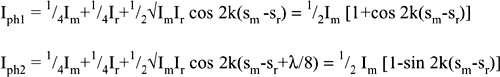
Now, with the pair of cosine and sine interferometric signals, the argument s_m-s_r of the trigonometric functions can be recovered without ambiguity. One possible processing strategy is illustrated in Fig.4-4.

Fig. 4-4 Signal handling in a two-beam interferometer. Cosine and sine signals are passed through discriminators, logic signals of amplitude and slope are obtained, and an appropriate logic combination of them acts as the up/down command at the counter input.

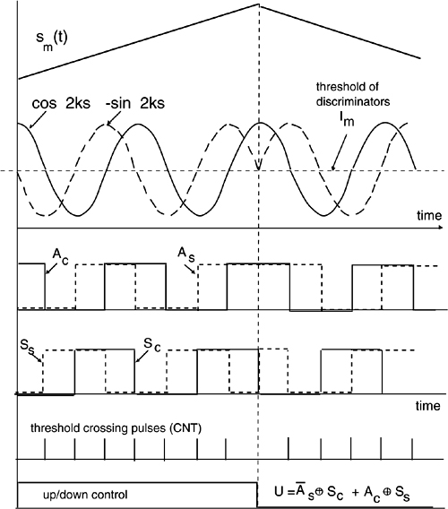
Fig. 4-5 The up/down 7-decade decimal counter stores the displacement under measurement in λ/8 units. A 6-digit multiplier brings the reading to metric units for the buffer register and the display.

Each signal out from the photodetector is passed through a comparator, with the threshold placed at the average (½ I_m) photocurrent so that amplitude logic signals A_C and A_S are generated (A=1 for high amplitude, A=0 for low amplitude).

Next, slope logical signals S_C and S_S are generated for each channel, according to the sign of the signal slope (S=1 for positive slope, S=0 for negative).

Count pulses are generated for the switching of both sine and cosine signals, for example, by differentiating the discriminator’s outputs (either upgoing or downgoing) and by rectifying the obtained pulses so that they are all positive. Because the sine and cosine signals provide four switchings per λ/2-period, one count represents a λ/8 (=0.079 μm for a 633-nm He-Ne laser) increment of displacement s_m.

Count pulses are sent to an up/down counter as clock (or count) pulses, and a logic combination of amplitude and slope enables the up/down input in the correct direction. With reference to Fig.4-4, let us suppose that the displacement first increases and then decreases. At the first switching, it is A_S=0 and S_C=0, at the second A_C=0 and S_S=1, at the third A_S=1 and S_C=1, and at the fourth A_C=1 and S_S=0, whereas in the decreasing portion the reverse is true.

The appropriate logic for the up-count command is therefore written as:

(4.6)

where * stands for the negation (or complement) and ⊕ for the exclusive-or logic operation. The calculation of U is easily implemented by using a few logic gates, as shown in Fig.4-5. The counter is normally a 7-decades counter, so that it can nominally accommodate readings of displacements from 0.079 μm up to 0.79 m.

Now, after the counter, we shall bring the counter content to decimal. This requires a 7-digit multiplier, with the other number entering the multiplier being the length corresponding to one count, e.g., 791..…, usually settable in a register for calibration.

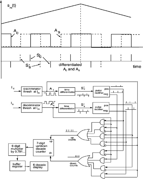
Fig. 4-6 Another more robust strategy for pulse counting in a two-beam interferometer. Pulses S_c’ and S_s’ from the switching edges of the discriminator outputs are processed directly by the AND/OR gates, and the results are counted in a 7-digit up/down counter.

The result is stored in a 6-digit buffer register, which has 0.1-μm as the least-significant digit and 0.1-m as the most-significant digit. Therefore, a displacement up to ±0.999999 m can be measured. The buffer is connected to the numeric display. This allows the display to be refreshed periodically (e.g., every 0.1 s) and to avoid the last digits from changing fast and becoming unreadable during count buildup. It is not advisable to go beyond 6 digits because of several errors intervening at the ppm (or 10^-6) resolution level.

The processing scheme described previously works well with well-behaved displacement waveforms, but has a weak point. The slope logical signals S_S,C are obtained necessarily by a high-pass circuit that rejects quasi-dc components of I _ph1,2. We can indeed design it with a very low frequency cutoff covering the practical range of s_m(t) expected frequency content, but can never reach zero. Therefore, an objectionable possible loss of counts for very-slow waveforms s_m(t) remains.

This drawback can be overcome with the more robust processing scheme of Fig.4-6. Here, we perform the up/down logic operation directly on the switching signal edges, derived from the amplitude comparator outputs, which make the same logic function as described by Eq.4.6, but without the need for a slope logic signal. Accordingly, the scheme of Fig.4-6 removes the low-frequency constraints on s_m(t).

The position of the discriminator threshold, nominally set at ½ I_m in electronic processing, is a critical factor to the performance of the two-beam interferometer. Because the photodetected signals I_ph1 and I_ph2 (see Eq.4.5 and Fig.4-4) can go well below the average value simultaneously, the strategy to derive the threshold is not trivial, unless an assumption on the expected behavior of s_m(t) is made. Perhaps, the less stringent assumption is that, because of ambient-related vibrations, s_m(t) undergoes several λ-cycles in a medium-term period. Then, a good practical choice is to take the threshold as the semisum ½ (I_ph1+I_ph2) of the interferometric signal amplitudes, integrated on say, a 1-s period.

Regarding the high-frequency cutoff of the circuits, if we take all of them having at least (a specified) bandwidth B, the interferometer can correctly count λ/8 steps of displacement at a rate of one per period 1/B. The maximum velocity allowed to target displacement is then: v_target= (λ/8)B. For B=10 MHz and λ/8=0.079 μm, we get the quite satisfactory value v_target= 0.8 m/s.

When going to the field, the two-beam interferometer is recognized as satisfactory by users. However, it reveals the following drawbacks that need to be eventually corrected:

- If the optical beam is interrupted, counts are lost and the measurement run shall be repeated

- High-frequency (EMI) disturbances sometimes leads to counting errors.

- Ambient-induced vibrations can occasionally lead to incorrect counts.

For the first point, a strategy is to monitor the amplitudes of signal I_ph1 and I_ph2 and give a warning (with a panel-mounted LED) when both fall below, say 5% of the time-averaged threshold.

The second and third points call for a good shielding from electromagnetic, as well as mechanical disturbances, but are difficult to be eliminated intrinsically. The basic reason is that the two-beam interferometer works on threshold crossing by baseband signals. Thus, all the disturbances falling in a spectral range 0-B are indistinguishable from signals and, even if small in amplitude, may lead to incorrect switching of the discriminators.

4.2.2 The Two-Frequency Laser Interferometer

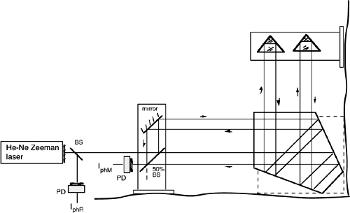
In this approach, we take advantage of the frequency difference between the two-orthogonal polarization modes emitted by a Zeeman-stabilized He-Ne laser (see App.A1.1.3) to make the interferometric signal available on a carrier frequency instead in baseband.

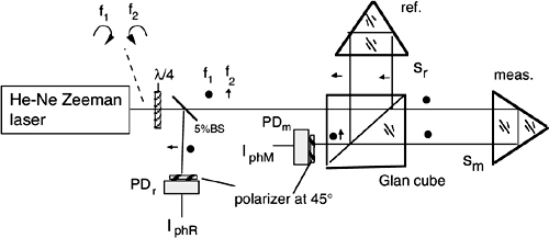
The basic schematic of the two-frequency interferometer is reported in Fig.4-7. The Zeeman laser is one with an axial magnetic field and generates two counter-rotating, circularly polarized modes, that are spaced in frequency by f₁-f₂=5 MHz approximately. The circular polarizations are transformed into linearly polarized waves by a quarter-wave retarder inserted at the laser output.

Before entering the optical interferometer, we first get a reference signal I_phR at the frequency difference f₁-f₂. To do so, a small fraction η of the beam power (for example, η≈5%) is deviated to the reference photodiode PD_R, in front of which a polarizer oriented at 45° is placed. The photocurrent is therefore written as (cf. with Eq.4-2):

(4.7)

where φ=φ₁−φ₂ is the relative phase of the two modes, and we let I₁=I₂=I_av for simplicity.

In the optical intereferometer, we use the usual corner cubes and a Glan-cube beamsplitter (or polarization splitter), one with the property of dividing linear polarizations. The Glan is usually made by calcite, a well-known birefringent crystal. The two halves of the Glan are cut along different orientations of the crystal, to have a large difference of index of refraction for the two polarizations. In this way, at the separation surface, incidence is beyond total reflection angle for one polarization (the perpendicular to incidence plane), which is accordingly reflected, while it is below the total reflection for the other polarization (the parallel to incidence plane), which is transmitted.

Thus, by virtue of the Glan-cube splitter, we are able to direct one polarization (the perpendicular, at frequency f₁) along the reference path, and the other (parallel, f₂) to the measurement path. On the return path, the two polarizations recombine in a beam directed on the photodetector (Fig.4-7).

In the propagation to the corner cubes and back, the two waves have cumulated a phase shift 2ks_m and 2ks_r and, accordingly, the signal I_phM from the photodetector PD_M is:

(4.8)

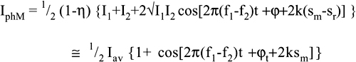
Fig. 4-7 The two-frequency interferometer uses the two modes of a Zeeman laser, separated by f₁-f₂≈5 MHz and with orthogonal polarizations. The polarization Glan beamsplitter sends one mode to the reference path and the other mode to the measure path. Upon recombination, the phase difference 2k(s_m-s_r) is found on the carrier frequency f₁-f₂.

where we have taken I₁=I₂=I_av, neglected the small η, and let φ_t=φ+2ks_r for the phase term, which is a constant if 2ks_r is kept constant.

Eq.4.8 shows that the quantity to be measured, 2ks_m, is now a phase superposed on a carrier at frequency f₁-f₂. To recover it, we have several possible choices.

For example, we may want to go back to analog interferometric signals. Then, we can electrically mix the photodetected signals I_phM and I_phR and generate sum-and-difference frequencies. The difference frequency term is cos 2k(s_m-s_r) and is recovered with a low-pass filtering of the mixer output. Also, by phase-shifting the reference I_phR by π/2 and mixing it again to I_phM, we obtain sin 2k(s_m-s_r). This approach works, but does not fully exploit the advantages of the two-frequency arrangement, which are made clear later.

A better signal processing is illustrated in Fig.4-8. The photodetected signals, I_phM and I_phR, are squared by comparators and, from the transitions (e.g., positive going), one pulse per period is obtained. We use two counters, one for the measurement and the other for the reference channel. The counters are allowed to count freely, and their content is transferred to buffers registers by a gate pulse G1. This pulse has a period T, which is the renewal time of measurement (typically 0.1 s). The reason for the buffer registers is that pulses may occur simultaneously in the two channels, both running close at f₁-f₂≈5 MHz, and they cannot be handled directly by an up/down counter (unless we use a complicate logic circuit).

To find the content of the counters at the end of period T, we use Eqs.4.7 and 4.8 with (d/dt)φ_t =0, i.e., assume a still reference-arm. Also, we recall that frequency is the time derivative of the phase, f=(1/2π)dφ/dt, and that counters perform an integration operation, which yields the integer part of the quantity C= ∫_0-Tf dt.

Thus, we obtain:

(4.9)

In this equation, v_m=(d/dt)s_m is the velocity of the measurement-arm corner cube. The term v_m/λ in the second line of Eq.4.9 can be recognized as the change in frequency induced by the Doppler effect, usually written as Δf=(v/c)f. The term Δs_m in the last line of Eq.4.9 is the displacement occurred in the period T, in units of λ/2.

The subtractor (Fig.4-8) makes the difference of the buffer contents, and the result is:

(4.10)

Last, the content of the subtractor is transferred to the main output register by the gate pulse G2 (delayed respect to G1, see Fig.4-8, to allow for subtraction time). In the output register, the 2Δs/λ counts from the subtractor are added (with sign) to the content already present there. Thus, the content at time t represents the counts in λ/2 units of s=∫_0-τΔs, which is the total displacement from time t=0 (the general reset) to current time t.

Fig. 4-8 Signal processing for the two-frequency interferometer. Measurement and reference signals are counted for a period T, and then are transferred to buffers. The results are subtracted to yield 2kΔs. A main adder gives 2ks, and a multiplier converts the counts in decimal units for the display.

The measurement resolution is now λ/2, but we can bring it readily to λ/4 by doubling the pulses obtained from the comparators (that is, by adding the negative-going transitions in both channels, properly rectified).

In a two-frequency interferometer, the maximum speed of the corner cube we can follow with correct counts is again v=(λ/4)B, where B is the bandwidth of processing circuits and, also, of the signal I_phM and I_phR filtering around the carrier f₁-f₂=5 MHz.

Allowing for a reasonable fraction of the carrier frequency, i.e., B=1MHz, we get a speed limit typically about v=0.15μm·10⁶s^-1=0.15 m/s.

The advantages of the two-frequency method over the two-beam method can be summarized as follows:

- The threshold of discrimination can be placed at zero because the dc components of I_phM and I_phR can be removed without loss of information.

- The rejection of electromagnetic disturbances is much better, at the 5±1 MHz frequency, as compared to the baseband.

- Any beam loss or interruption is readily detected, looking at the I_phM signal amplitude.

Fig. 4-9 A typical laser-interferometer instrument (from [2], by courtesy of Hewlett Packard)

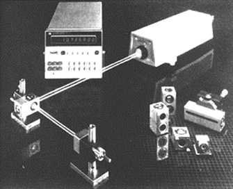
Based on the two-frequency approach, a number of commercial laser interferometers have been developed and are available from several vendors worldwide. Perhaps the most popular has been the 5525 Hewlett-Packard “Laser Interferometer”’ (Fig.4-9). This instrument was first released in 1967 and can nowadays been considered a great commercial success of electro-optical instrumentation.

4.2.2.1 Extending the displacement measurements to nanometers

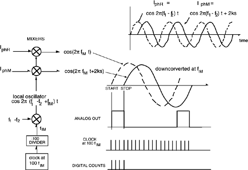
Also, we can go well beyond the λ/4 resolution and down to the ultimate limits of sensitivity by means of an electrical phase-shift measurement performed directly on the I_phM and I_phR waveforms, as illustrated in Fig.4-10.

To do so, it is customary to electrically mix both signals with a local oscillator at a frequency f_LO=(f₁-f₂)-f_IM, where f_IM is the intermediate frequency (usually f_IM ≈ 10-100 kHz) at which we perform the electrical phase-shift measurement. A feature interesting to be noted is that the phase shift 2ks is transferred from the f₁-f₂ carrier to a lower intermediate frequency f_IM with no error.

By measuring the phase shift with a 100-interval subdivision of the 2π angle, as provided by a counter at 100 times the intermediate frequency, we obtain a λ/200 resolution from the interpolator.

Fig. 4-10 The concept of interpolation to extend the resolution to λ/200 in a two-frequency interferometer.

The output of the interpolator is in digital format and is suitable for supplying the user with two additional decades of counts, that represent, say 0.01 and 0.001 μm.

Alternatively, we may also amplify and low-pass filter the analog output of Fig.4-10 to make available an analog-format signal that supplements the digital readout for small displacements.

It is interesting to remark that a nm-resolution of a displacement measurement is seldom required in machine-tool applications and, if we actually want to attain it, operation of the instrument on an antivibration table is mandatory.

On the other hand, measurement of vibrations (that is, periodic phenomena) with amplitudes down to nanometers and picometers really makes sense and has been actually developed (see next sections). The oscillating character of the phenomenon can be used to develop much simpler and effective approaches.

We may also wonder if the two-beam interferometer can be extended to operation in the nanometer range. Trying to resolve a submicrometer displacement Δs from the two signals given by Eq.4.5 leads to an ambiguity. Indeed, the signals X=1+cos2ks and Y=1-sin2ks lead to a second-degree equation in the argument 2ks.

To remove the ambiguity, we need at least to triplicate the measurement channels of the interferometer. One of the possible methods [6] is illustrated in Fig.4-11. It consists of segmenting the propagating beam aperture in three sectors, each detected by a separate photodetector. On the propagation path, a segmented retardance plate is inserted, with 0, 120, and 240 degrees of retardance. Thus, the signals are:

where A allows for nonunitary fringe contrast. By combining the signals, we have:

(4.11)

Now, the term 2ks can be solved for as: 2ks= -atan This calculation requires a small microcomputer receiving the signals S_1,2,3 through an A/D converter interface. In laboratory experiments [6], the approach has demonstrated to reach a 1-nm resolution easily.

Fig. 4-11 Extension of the two-beam interferometer to nm-resolution.

4.2.3 Measuring with the Laser Interferometer

The laser interferometer, in any of the previously described implementations, measures the incremental displacements of a target (the retroreflector). As such, it requires an initial reset (zeroing) of the counters with the target positioned on the mechanical zero of the system under control.

The target distance is dynamically measured by counts and requires that regular counts are developed and that no beam interruption occurs at any time during target movement. Interruption of the beam while the target is moving results in a loss of counts, and thus a wrong measurement that cannot be corrected anymore. In this case, we shall go back to the initial reset and restart operation.

For the same reason, immunity of the instrument to Electro-Magnetic Interference (EMI) is of the utmost importance, because we have no way to discriminate spurious EMI pulses from true displacement pulses. Interference may result in a wrong measurement with no warning to the user.

Another source of spurious counts comes from microphonics. This term means sensitivity to ambient-related mechanical disturbances that induce vibrations into the measurement path. Vibrations generate up/down counts that have nominally zero average and are harmless, but may introduce an error when the content is sampled instantaneously.

In interferometers with fraction-of-λ resolution, vibration-induced spurious counts are kept low or negligible by mounting the measuring setup on a suitable antivibration table. On the other hand, if we deal with instruments reaching the nanometer resolution, mechanical isolation is more demanding and may require a special design or arrangement of the experimental layout.

Another specific requirement of the laser interferometer is the need for a corner cube reflector.

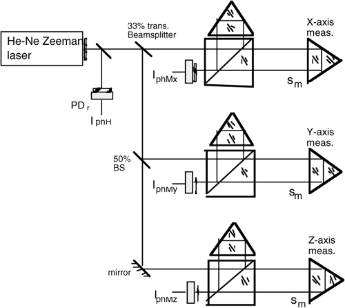
Fig. 4-12 Three-axis extension of the interferometer measurement

The corner cube is mounted on the moving carrier of the tool-machine under measurement to serve as the mechanical reference. The device is generally compact (typically, 1-2 cm in diameter), yet mounting it in the experiment means that the measurement is invasive. Additionally, we need to keep it reasonably clean in the surrounding environment.

In the practical operation of the instrument, several systematic errors may occur.

One is the cosine error, arising because the beam wave vector k and the motion vector s are not strictly parallel, but form an angle α_ks. As the target is moved, the displacement s is measured as if it was s cos α_ks. To adjust the parallelism of k and s, despite vector k being immaterial, we must check alignment of an optical component (usually the front surface of the corner cube) at the beginning and at the end of a displacement stroke [3].

Another systematic error comes from minute spurious reflections of the reference and/or the measurement beams on a parasitic optical path. If ε is the fraction of optical power leaking to the unwanted path, either reference or measurement, a cyclic error is generated. This cyclic error is a ripple error, affecting the true value of measurement with an amplitude σ_cyc and a periodicity λ/2 versus displacement [4].

Using good engineering practice, the previous errors can be minimized and the laser interferometer can be used in a number of circumstances, as detailed in the following sections. Frequently, the ultimate limits of performance discussed in Sect.4.4 are actually reached.

4.2.3.1 Multiaxis extension

Tool machines with numerical control usually require three-axis positioning. We do not need to triplicate the interferometer to perform a three-axis measurement, however.

Fig. 4-13 A universal tool machine equipped with a three-axis laser interferometer (from Ref. [3], by courtesy of Hewlett-Packard)

To save parts, we may share the laser, taking advantage of the power being still adequate when reduced to 1/3, and use for each axis the two-frequency scheme, with the same reference for all axes, as illustrated in Fig.4-12.

A universal tool machine equipped with the three-axis laser interferometer is shown for illustration in Fig.4-13.

4.2.3.2 Planarity measurement

Another measurement commonly performed in mechanical workshops is planarity.

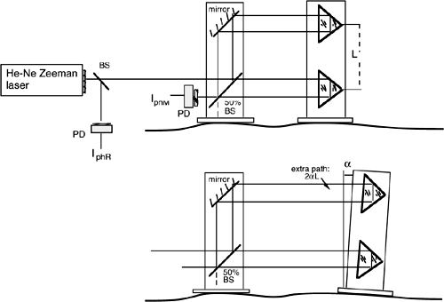
We may use the scheme shown in Fig.4-14 where, by aid of a beamsplitter and mirror combination, we direct two beams to a couple of corner cubes mounted on a square.

The square with the corner cubes is moved along the plane to be tested, whereas the reference mirror and beamsplitter assembly is kept fixed.

The measurement photodiode receives the recombined beams returned from the corner cubes, and it supplies a signal containing the interferometric phase difference 2k(s_upper-s_lower), where s_upper and s_lower are the path lengths of the upper and lower beams.

When the corner cube square is moved and it remains parallel to itself, s_upper and s_lower increase by the same amount, and no count is developed. However, if a tilt α is suffered, the path length difference 2αL is counted in units of λ/4, with L being the distance between the corner cubes (Fig.4-14). Thus, the angular resolution corresponding to a single count is α_1c = λ/8L. Taking L=100 mm and being λ=0.633 μm, we get α_1c =0.8 10^-6 rad or 0.16 arc-sec, a very good resolution indeed.

Fig. 4-14 Planarity measurement scheme

As a further step, we may divide the surface under test in individual cells, typically of the size of the corner cubes square basement, let’s say L_B=100 mm, and collect the measurement counts N_c developed along the surface.

From these data, the profile z(x,y) of the surface under test can be easily computed as a function of spatial coordinates x and y simply by adding step by step the vertical displacement Δz=αL_B=N_cL_B λ/8L from one cell to the next.

The vertical resolution we obtain in the planarity deviation of the surface under test is Δz=N_cλ/8 (for L_B=L), or, λ/8=0.08 μm using a He-Ne laser interferometer.

4.2.3.3 Rectangularity measurement

A variant to the planarity scheme is obtained by adding a 90° deviation of the beams by means of a pentaprism, as indicated in Fig.4-15.

The pentaprism has a dihedral angle of γ=45°, and it is easily seen to deviate the incident beam by 2γ=90° irrespective of the incidence angle. With respect to using a mirror oriented at 45°, the pentaprism eases the alignment and introduces no error associated to incidence angle.

The counts developed in the arrangement of Fig.4-15 are related to the planarity errors, plus the deviation error from rectangularity of the surface under test on which the mobile corner cube square slides on.

Again, the resolution in rectangularity is the same as for planarity, α_1c=λ/8L, while the precision, is of course, affected by the pentaprism dihedral angle error ε=γ-45° (typically <1 arcsec in best units).

Fig. 4-15 Rectangularity measurement scheme

4.2.3.4 Extending the measurement on diffusing targets

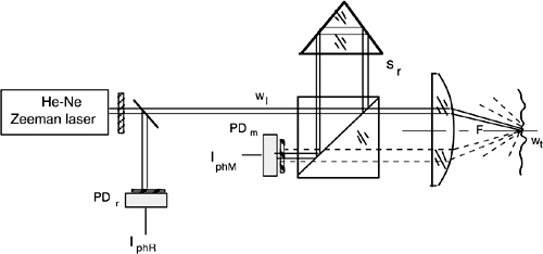
Still another extension of the basic interferometer, either dual-beam or two-frequency, is that of attempting operation on diffusing surfaces. To improve collection of light returning to the measuring section, we need a focusing lens in front of the diffusing target that is used in place of the corner cube, as shown in Fig.4-16.

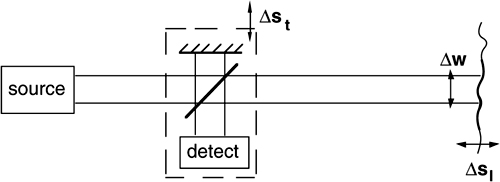
Though the scheme in Fig.4-16 is probably not the optimal approach, it is instructive to analyze it to point out the problems we face using a diffuser. On the target, the spot focused by the lens ideally has a (radial) dimension w_t=λ/πNA (see Eq.A2-10 in Ref.[5]), where NA is the numerical aperture of the lens used by the incoming beam, given by NA= w₁/F, where F is the lens focal length and w₁ the input beam spot size.

Radiation rediffused by the target follows Lambert’s law (see [5], Appendix A2) and the amount of it superposed to the reference path spot of area πw₁² on the photodiode PD_m is readily found as P_m= (1/π)P₀(πw₁²)/F²=P₀(w₁/F)² where P₀ is the power from the laser leaving the beamsplitter. Because it is usually (w₁/F)²<<1, first we shall expect a weak signal back to the readout section of the interferometer.

This is not a serious problem, however, because the interferometer detection is a truly coherent detection scheme (see [5], Sect.8.1) and, accordingly, it works at the quantum limit of the received power. When the target moves, a signal of the form 2ks is developed, that can be processed like in a conventional interferometer, even though its amplitude is attenuated by w₁/F with respect to the signal from a corner cube target.

Of more concern is the range of displacement allowed for the measurement before a large speckle error is suffered.

When the diffuser moves along the z-axis appreciably, it runs out of focus with respect to the (fixed) lens.

Fig. 4-16 Modification of the optical setup for operation on a diffusing target

The size of the spot w₁ then increases and, much worse, the sample of random elemental areas contributing to the returned field also changes, adding a random phase error φ_sp to the expected phase shift 2ks.

This error is called the speckle-pattern phase error, and it will be analyzed in detail in Section 5.1. For the moment, let us just mention that φ_sp becomes comparable with 2π as the displacement Δz brings the target out of focus of the lens. As a consequence, the diffuser statistical sample generating the speckle is changed over, and the phase error is ≈2π.

For this to happen, we need Δz=w_t/(w₁/F) where w₁/F=NA is the numerical aperture used by the beam of spot size w₁. Using w_t=λ/πNA in this expression, we get Δz =λ/πNA² as the dynamic range of maximum displacement for a λ-error. Even at a small NA, the resulting range is clearly much less than the tens of cm to meters we require in applications of the interferometer to mechanical metrology.

On the contrary, the dynamic range allowed by the speckle statistics is adequate for vibration measurements, where the amplitude of the periodic displacement is much smaller (typically ranging from nm to hundreds μm).

4.3 Performance Parameters

Irrespective of the working principle, interferometers can be characterized by a set of parameters describing their ability to detect target movement in a variety of situations.

The first is the minimum detectable amplitude of displacement that is set either by a threshold of discrimination or by the noise inherent to detected radiation or to circuits.

Second, the maximum amplitude of displacement that is accommodated is limited by the dynamic range of circuits.

Third, we find a maximum (and eventually, a minimum) frequency of detectable displacement due to the frequency cutoff B of the circuits handling the interferometric signal.

Last, we shall consider a fourth limitation – the speed or Doppler limit – due to the fact that even a slow displacement can develop a high-frequency interferometric signal. Indeed, if the target moves at a speed v, the interferometric signal is cos2ks=cos2kvt, or its frequency content is f=2kv/2π=2v/λ. This quantity shall be less than the circuit bandwidth B, indicating that large and fast displacements have a v<λB/2 limitation in performance.

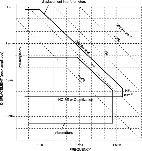
We can represent these four parameters in a diagram of performances (Fig.4-17) which is also called Wegel’s or lemon diagram because of its shape. Each square in the diagram is a 10 by 10 factor of covered performance. The more decades found in the diagram, means the more the instrument performs.

Of course, several other parameters are necessary to complete the interferometer performance description. The most common are the following:

(i)   The accuracy of the readings (depending on the calibration and stability of the wavelength).

(ii)  The dependence on temperature and atmospheric pressure and composition

(iii) The dependence on quasistatic magnetic fields.

(iv) The immunity to EMI disturbances.

Fig. 4-17 Wegel’s diagram for interferometer performances. Operation is inside the thick-line perimeter. Typical performances of a displacement-measuring interferometer and of a vibrometer are indicated.

4.4 Ultimate Limits Of Performance

We have seen in the preceding sections that laser interferometers easily reach several digits (e.g., six) of dynamic range and submicrometer resolution. To ascertain the fundamental limits of operation posed by physical laws, we analyze in this section several factors that affect the instrument performance.

4.4.1 Quantum Noise Limit

The ultimate limitation to the sensitivity of a laser interferometer is the quantum limit associated with the detection of the signal returning from the optical interferometer.

Let us consider it in detail, starting with the photocurrent written in the generalized form as:

(4.12)

where R is the responsivity and V the fringe visibility (see App.A2). For simplicity, the reader may start taking V=1 and R=2, as in previous sections.

We assume that we can adjust the reference path so that the interferometer works in a quiescent point of maximum sensitivity, that is at Rk(s_m-s_r)=φ-π/2 (or, at half fringe). In this case we have from Eq.4.12:

Explicitly, the phase φ will then be given by the small displacement to be measured, φ=RkΔs. For a small deviation around the quiescent point, the photocurrent deviation ΔI_ph is:

(4.13)

Superposed to the useful signal I_ph, we find a fluctuation ΔI_ph associated with the shot (or quantum) noise (see [5], App.A4) of the quiescent point current I₀. The rms value i_n of such noise is proportional to the square root of the average current I₀ and of the observation bandwidth B:

(4.14)

The associated signal-to-noise ratio of the current amplitude measurement around I₀ is S/N= i_n/I₀ = (2eB/I₀)^1/2. Equating φ=φ_n and ΔI_ph = i_n in Eqs.4.13 and 4.14, we get:

(4.15)

Now, we may introduce the Noise-Equivalent-Displacement (NED) which is defined as the value of displacement Δs giving the same effect as the intrinsic noise φ_n. By definition and Eq.4.12, it is RkΔs = φ_n or:

(4.16)

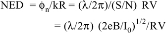
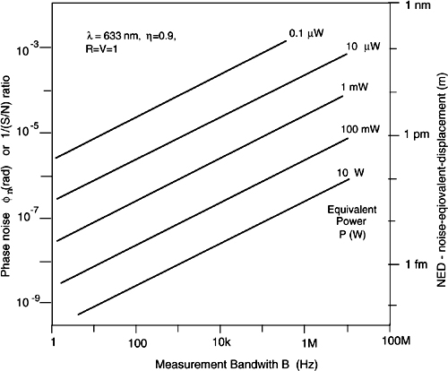
The diagram of Eq.4.16 is plotted in Fig.4.18 for the representative case of λ=633nm, η=0.9, and R=V=1.

As we can see from the figure, the quantum limit is indeed very low and theoretically allows us to reach very high sensitivities (e.g., φ_n≈10^-6-10^-8 rad in most cases).

For example, a displacement sensor working with an instrumental bandwidth of, say, B=1 Hz, and with 1mW of detected power, we can go down to a resolution of just a few femtometers (10^-15 m). For a vibrometer aimed at detecting oscillations up to a few hundred kHz, the quantum noise limit is around a few picometers (10^-12 m).

These very challenging figures are indeed obtained in practice, for example, in the gyroscope. However, we shall stress that generally they require a very careful design to first get rid of several perturbing effects, usually much larger than the quantum limit.

For RV ≠1, the values of φ_n read in Fig.4.16 shall be divided by V, the fringe visibility, and those of NED by RV.

Fig. 4-18 The phase noise and the NED versus measurement bandwidth B, with the detected power P as a parameter, at the quantum noise limit of operation in an interferometer

4.4.2 Temporal Coherence

When recombining two beams propagated on different lengths along the measurement s_m and reference s_r paths, we actually superpose two field contributions delayed of a time T=(s_m−s_r)/c. If the optical frequency ν is not truly constant, but fluctuates in time, a decrease from the ideal unity visibility of fringes is incurred, and additionally, a phase error in the measurement of k(s_m−s_r) is generated.

An easy way to describe the decrease of fringe visibility is to consider the finite line width Δν of the source. If frequency ν₀ is defined not better than Δν in the time-dependent term exp i2πνt+iφ= exp i2π(ν₀+Δν)t+iφ, after a time T_coh= 1/Δν the initial phase φ has changed by 2π, and coherence is lost (see also Appendix A1.1.2).

Time T_coh is therefore called the coherence time of the source. Alternatively, we talk of coherence length L_coh=cT_coh as the distance traveled by light in the coherence time T_coh. The quantity L_coh represents the maximum value allowed to the path length difference s_m−s_r of the interferometer if a beating is to be obtained.

Usually, if the shape of the line is a Lorentzian, p(ν)=[1+4(ν-ν₀)²/Δν²]^-1, the decrease of fringe visibility is a negative exponential: A=exp-T/T_coh.

To study the phase error due to incomplete temporal coherence, let us assume that the frequency is a constant ν₀ and ascribe all the fluctuations to the phase term φ(t). Writing the superposed fields as:

The beating on the photodetector becomes:

(4.17)

Now, let us express the phase term φ(t)=φ₀+φ_n(t) as the sum of a mean value φ₀ and a random fluctuation φ_n(t) with zero mean value, or φ_n(t)=0. Then, the phase difference in Eq.4.17 becomes φ(t)-φ(t+T)=φ_n(t)-φ_n(t+T)= φ_n and we get by inserting in Eq.4.17:

(4.18)

The mean photodetected current is obtained by taking the average at both sides of Eq.4.18. Because φ_n=0, it is also sin φ_n=0 because sin φ_n is an odd function of a zero mean argument, and therefore we have:

where μ_tc=cosφ_n takes the meaning of coherence factor (see also [5], Sect.8.1.2). Developing the cosine in Taylor’s series, cosφ_n=1-φ_n²/2+…, reveals that μ_tc≈1-φ_n²/2 is related to the variance σ_φ²=φ_n² of the random-phase difference φ_n(t)-φ_n(t+T) at times t and t+T. If T is short, we may expect that φ_n keeps much less than unity and μ_tc≈1. The fringe visibility then decreases as A=μ_tc in Eq.4.12.

Moreover, the fluctuation i_n around the mean value I_phadds a phase error. To evaluate it, let us note first that the cosφ_n term in Eq.4.18 is close to unity, in the case of practical interest of not so bad temporal coherence (μ_tc≈1), and therefore it can be assumed as a constant not contributing to fluctuations. By taking the differentials at both sides of Eq.4.18, and then squaring and averaging, we get for the variance i_n²:

Again assuming the case of μ_tc≈1, the term sin²φ_n can be approximated to φ_n²=σ_φ². Now, we recall that the phase error is related to the amplitude error by Eq.4.15, and assume that the maximum sensitivity condition k(s_m-s_r=-π/2 to obtain the result:

(4.19)

The phase error σ_φ²can be traced to the two-sample Allan’s variance σ_ν²(2,T,τ) describing the frequency stability of a generic oscillator. This quantity is defined as:

(4.20)

or, it is the mean square deviation of two frequency samples separated by a delay T and averaged on a time interval τ. The phase error is found to be related to the frequency variance by σ_φ=(2πτ)σ_ν(2,T,τ), and in its turn σ_ν is related to a two-consecutive sample variance by σ_ν(2,τ,τ)=τ/T) σ_ν(2,T,τ) for T<< τ.

Using Eqs.4.16, 4.19 and 4.20, we then get the NED_tc due to temporal coherence effects as:

Recalling that T=(s_m−s_r)/c, we may write the result in the expressive form:

(4.21)

This result tells us that incomplete temporal coherence, beyond reducing the fringe visibility, produces a noise-equivalent random error equal to a fraction of the arm mismatch (s_m−s_r). The fraction is given by the relative frequency stability σ_ν/ν of the source and is evaluated in the integration time τ (where τ =1/2B in terms of observation bandwidth).

With practical frequency stabilized lasers, frequency stability of 10^-9 to 10^-11 are obtained, so a 1-count or λ/4=0.15 μm error is generated for an arm mismatch s_m−s_r= 0.15 μm/(10^-9..10^-11)≈0.15..15 km.

4.4.3 Spatial Coherence and Polarization State

In the superposition at the photodetector, the reference E_r and measurement E_m fields shall have the same spatial mode distribution. If not, their interference term, and according the fringe visibility, will be reduced from the full value to a factor:

(4.22)

Eq.4.22 explains why interferometers shall use single-mode beam spatial distributions. If the beam contains a mixture of N modes sharing the total power, because the integral product of different modes is zero, only homologous modes will contribute to μ_sp. The net result is that μ_sp cannot be larger than 1/N. More commonly, it will be μ_sp<<1/N because, in addition, the different modes may have a slightly different propagation constant and smear out the interferometric phase difference.

Similarly, we shall use the same State of Polarization (SOP) for both modes, either linear or circular, or generically elliptic. If not, the signal will be reduced by a factor:

(4.23)

where E_m·E_r is the product of Jones matrixes of signal E_m and local oscillator E_r, and |..| indicates the modulus of vectors.

Thus, the combined effect of spatial, temporal, and polarization matching is to reduce the fringe visibility to:

(4.24)

No extra noise is generated by the loss of visibility due to spatial and polarization effects, however, because of the deterministic nature.

4.4.4 Dispersion of the Medium

A nice feature of interferometric measurements is the very precise yardstick on which they are inherently calibrated: the wavelength. However, we usually propagate the beams in air, and therefore the unit of measure is λ/n_air. Though not too different from unity, the index of refraction can indeed introduce a calibration error in measurements with several significant digits.

In standard condition (T=15°C and p=760 mbar) and with its standard composition, air has an index of refraction that is well approximated by the following expression (see Ref.[7] of Ch.3):

(4.25)

We can see from this expression that in standard conditions the interferometric measurement requires a correction of about 280 ppm (ppm = part-per-million) at λ=633 nm. In addition, the correction is also dependent on the wavelength of operation, and the amount is a few ppm along the visible to near infrared regions.

At temperatures and pressures other than those of the standard conditions, the excess to 1 of the index of refraction is easily computed by noting that this quantity is proportional to the mole number per unit volume n/V, and therefore is equal to P/RT for the law of perfect gases. Therefore we can write:

(4.26)

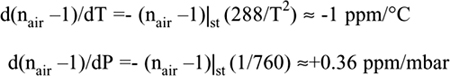
From Eq.4.26 we can calculate the temperature and pressure coefficients of the wavelength and of the correction to the corresponding interferometric measurement:

(4.27)

If we take reasonable values for ΔT and ΔP, for example 10°C and 10 mbar, we can see that temperature and pressure variations affect the 5^th and 6^th decimal digits of the displacement measurement. As already noted in Sect.4.2.1, the correction is performed by two sensors with outputs that change the multiplication factor (as shown in Figs.4-6 and 4-8) used to convert the fraction-of-λ counts to a metric scale.

Ideally, the sensors should average T and P on the actual optical path, but this is clearly awkward in practical operation.

With point sensors, located internal to the instrument, or close to the measurement optical path covered by the instrument, the correction is effective to the 6^th decimal digit in the normal laboratory conditions.

4.4.5 Thermodynamic Phase Noise

In optical fiber sensors with interferometric readout (see App.A2 and Fig.8-28)), the thermodynamic fluctuation of index of refraction of the fiber introduces a phase noise φ_th that may become comparable or even larger than quantum noise. By an analysis of the phenomenon [7], the NED_th is found as:

(4.28)

where k_B is the Boltzmann constant, T the absolute temperature, L the fiber length, and κ the thermal conductivity. Because of the interference of counter-rotating waves sharing the same medium, the Sagnac configuration (App.A2) provides a partial cancellation of φ_th and the best immunity to thermodynamic phase noise [7].

4.4.6 Brownian Motion

When aiming to small-mass targets, Brownian motion may add a fluctuation that has to be taken into account in interferometric measurements of vibrations or displacements, despite not being a fault of the instrument.

On the line of sight along which we are performing the measurement, we find a thermodynamic degree of freedom and hence an energy (1/2)kT. This energy shall be equated to kinematic energy (1/2)mv², thus obtaining:

(4.29)

In the same way, for a rotating target for which we want to measure the angular speed of rotation Ω, we have a kinematic energy (1/2)IΩ², where I is the inertia momentum of the target. Equating to (1/2)kT gives a variance of the angular speed:

(4.30)

Letting numbers in Eqs.4.29 and 4.30 reveals that even for not so small masses (e.g., 1 to 10 g), the Brownian-induced speed or displacement may become comparable to the quantum noise NED.

Example. If we let T=300 K and being k= 1.38^.10^-23J/K the Boltzmann constant, we get for a 1mg mass from Eq.4.29: v²=4^.10^-21/10^-3=2^.10^-18, or , which is a value well in the reach of a typical interferometer (it corresponds to s=1nm and f=1Hz in the diagram of Fig.4-17). Also, for a disk of mass 0.01-g and radius 1-mm, the inertia momentum is I=(1/2)mr²=5^.10^-3.10^-6=5^.10^-9, and we get from Eq.4.30: again a value within the readout sensitivity of a gyroscope (see Ch.7).

4.4.7 Speckle-Related Errors

When the interferometer works on a diffusing surface, a random phase error originates form the speckle-pattern statistics.

In addition, we find fading of field amplitude, as well as a deterministic field-curvature error. When these effects are cured, we are left with the speckle-induced phase error discussed in this section.

Of course, this situation is relevant only for the detection of vibrations on nonreflective surfaces, whereas in a corner cube interferometer the error is absent.

The statistical properties of the speckle field will be treated in Chapter 5. To discuss the ultimate error of an interferometric measurement on a diffuser, we refer to the conceptual scheme of Fig.4-19 (similar to the practical setup of Fig.4-16).

The three basic contributions to speckle errors, according to the displacement considered, are the following:

Fig. 4-19 Conceptual scheme to evaluate the NED of an interferometric measurement performed on a diffusing surface

(i)  On-axis (along the line of sight)

(ii)  Transversal (perpendicular to the line of sight)

(iii) Projection (change of the diffuser portion illuminated by the beam)

For a longitudinal displacement Δs₁ of the target along the line of sight, the noise-equivalent displacement is found as (see also Sect.5.1):

(4.31)

where S₁=λs²/w² is the longitudinal speckle size, and C is a factor depending on the intensity of the particular speckle on which we are making the measurement.

If I(0) and I(Δs₁) are the intensities (or powers collected) at the extremities of the displacement Δs₁, and I is the mean intensity, we have the conditioned value of C:

(4.32)

On the other hand, if we disregard the intensity or are not able to choose a particular speckle, the average (in quadratic sense) of the error given by Eq.(4.31) corresponds to the free value of C:

(4.33)

As we can see from Eq.4.31, the error is of the order of the wavelength multiplied by the dynamic-range to speckle size ratio. The factor C is of the order of unity (up to Δs₁≈S₁) in the free measurement (Eq.4.33), but, if we choose a bright speckle with I(0) and I(Δs₁)≈ I(0) say K times larger than the mean intensity I the NED is decreased with respect to the free value of a factor .

For a transversal displacement Δs_t of the interferometer in the speckle field, one that should theoretically give a zero output, we get an error:

(4.31a)

Here, S_t=λs/Δw is the transversal speckle size, and C is again given by Eqs.4-32 and 4.33 for the free and conditioned measurements, with Δs₁ and S₁ changed to Δs_t and S_t.

Last, a projection error is generated when the diffusing target moves transversally of a quantity Δw across the spot size w, a situation that should theoretically give no output. Because the random sample of the diffuser is changed, a random error is generated, and the corresponding NED is:

(4.31b)

All the errors considered previously can be kept to a small value by narrowing the allowed range of displacement as compared with a characteristic length. This length is the speckle-sizes S₁ and S_t for longitudinal/transversal displacements, and the spot-size w for a diffuser change.

Because both transversal and projection errors are likely to occur simultaneously in a practical setup, it may be useful to note that their composition is quadratic, that is NED = (NED_tr²+NED_tp²)^1/2.

4.5 Read-Out Configurations Of Interferometry

The laser interferometer we have considered so far can be classified as an external configuration, and in applications it is by far the most commonly used configuration. In it, the laser feeds an optical interferometer external to the source, and from the recombination of the propagated beams, a signal I₀ cosΦ is provided, that is, an intensity signal carrying the phase information Φ=2ks (see Fig.4-20).

This is not the only possibility we have available to make an interferometric readout, however.

We may also think of using the mirrors of the laser itself as the optical interferometer, as shown in Fig.4-20. This is the internal configuration, which generates an output signal of the form I₀ cos Ωt, i.e., a frequency signal Ω proportional to the optical phase shift, Ω=χks, χ being a suitable constant. The internal configuration is put to advantage in the Ring-Laser-Gyro (RLG) version of the gyroscope (Ch.7).

A third configuration is the injection-modulation, or self-mixing, interferometer, (Fig.4-20, bottom). Here, the optical interferometer external to the source is absent, and we rely just on the interaction of the returned field from the remote target into the laser cavity field to produce a modulation of the emitted field related to Φ.

The self-mixing configuration generates interferometric signals in form of Amplitude Modulation (AM) and Frequency Modulation (FM) of the oscillation (or, laser field), which carry the driving terms cosΦ and sinΦ, respectively.

Fig. 4-20 Configurations of interferometry: external (top), internal (middle), and injection or self-mixing (bottom)

4.5.1 Internal Configuration

Let us consider a laser oscillating in a single spatial and longitudinal mode, for example, a 20-cm He-Ne tube with external mirrors (see App.A1-1). As we move one mirror by a small displacement Δs along the cavity axis, the oscillation frequency will change by:

(4.33)

This result is explained because the spacing of longitudinal modes is c/2L, where L is the mirror distance (see Fig.A1-1) and, for each λ/2-increase of the laser cavity length L, frequency changes by c/2L (and the order of the mode increases by 1). Therefore, the ratio R_f of frequency variation Δf to displacement Δs, called responsivity R_f, is given by:

(4.34)

By letting λ=0.633 μm and L=20 cm so that c/2L=750MHz, we get from the internal configuration the remarkable responsivity to mirror displacement R_f = 750 MHz/316 nm = 2.4 MHz/nm, which is a very high value.

However, we cannot measure optical frequency directly and, to exploit this result, we need a second mode to be used as a reference frequency so that the frequency shift Δf can be converted down to an electrical frequency.

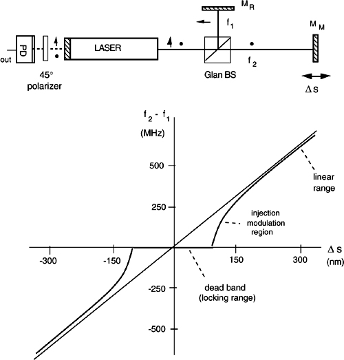
Thus, we have the arrangement of Fig.4-20, where a beamsplitter is used to allow the laser sustaining the oscillation of two modes, defined by the mirrors M_M and M_R. When M_M is moved, the frequency difference f₂-f₁ carries the interferometric signal and has a frequency variation proportional to Δs as given by Eq.4.34, a value that we will measure from the photodetector output. The maximum range of displacement is Δs=λ/2=316 nm, and the corresponding frequency is Δf= f₂-f₁=c/2L=750MHz. As we now have a Michelson interferometer brought inside the active cavity, the name internal configuration is justified.

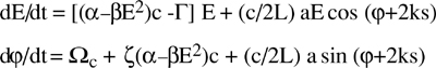
In an actual experiment, however, the linear response expected from the configuration is obtained only when the frequency difference f₂-f₁ is not too small (Fig.4-21). When f₂ approaches f₁, first a decrease in response is found, and then, for f₂≈f₁, the signal suddenly disappears [8,9].

The dead band is due to the frequency locking of the two oscillations. Locking is a very general phenomenon in coupled oscillators, which comes from even very minute coupling of power from one oscillation to the other. A residual very small interchange of power is unavoidable (for example, because of mirror scattering and gain-medium coupling), and therefore the dead band will never be zero (see also Ch.7).

However, we first try to reduce it as much as possible, and an improved scheme is shown in Fig.4-21. Here, because we use a Glan beamsplitter, two modes oscillate with linear orthogonal polarizations. At the rear mirror output, we can insert a polarizer in front of the photodetector, and orient it at 45° for the modes to beat on the photodetector.

Fig. 4-21 Internal interferometry. Top: scheme with polarization-split modes. Bottom: the theoretical response of frequency difference f₁-f₂ versus displacement Δs is linear, with a range of c/2L=750 MHz for a Δs =λ/2=316 nm displacement (values for a 30-cm He-Ne). In practice, a dead band around f₁-f₂=0 is found because of locking.

Because of the orthogonal polarizations, the gain coupling in the active medium is nearly suppressed. In addition, we get rid of the 50% loss of a normal beamsplitter used in Fig.4-20, which is hard to be compensated in a normal He-Ne laser.

Using low-scatter mirrors and a high-quality Glan cube to realize a He-Ne internal interferometer, we may go down to a few MHz of locking range as compared to several hundreds MHz of the basic scheme. Then, we can bias the interferometer to operate far away from f₂-f₁=0, e.g., at f_bias=100 MHz, so we can also detect the sign of Δs.

This can be done by finely adjusting the position of mirror M_R. A further refinement is to mount M_R on a piezo actuator and make a servo loop on the reference mirror position to stabilize the interferometer at f₂-f₁=f_bias=const. The Δs signal is then obtained from the error signal of the feedback loop.

The internal configuration is critical to operate because mirror M_M shall be kept aligned to the cavity during motion, and the tolerable error is much less than the diffraction limit, <1 arc-second in practice. Though the displacement we are aiming at might be very small, alignment is still very critical.

On the other hand, the internal configuration concept is useful in Sagnac interferometers like the gyroscope (Ch.7). In this case, optical path length variations are induced in a balanced cavity from outside, and the very high responsivity of the readout is put to great advantage.

4.5.2 Injection (or Self-Mixing) Configuration

Even without using any optical interferometer external to the laser source, we can make a laser interferometer by using the interaction, produced in the laser cavity, by a small fraction of the field emitted from a laser and returned back after propagation from the remote target.

First reported in 1978 [10], the resulting configuration is variously referred to in the literature as induced-modulation, injection, self-mixing, or feedback interferometry.

A straightforward explanation of the phenomenon comes from considering the field oscillating in the laser cavity as a rotating vector (Fig.4-22). The cavity field E rotates in the phase plane at optical frequency ω. If a fraction αE of it is allowed out for propagation to a remote target at distance s, the optical phase shift accumulated in the go-and-return path is Φ=2ks.

Thus, upon re-entering in the laser cavity through the mirror with transmittance t, we find a rotating vector of complex amplitude aE exp iΦ, where a=tαη, and η is an eventual propagation loss. This contribution adds as a vector to the existing field E to give the instantaneous new cavity field. The addition of rotating vectors is a well-known result of communication theory.

This result can be stated as follows. The in-phase component aE cos Φ produces amplitude modulation of the pre-existing field E, and its modulation index (or depth) is a·cos Φ. The in-quadrature component aE sin Φ produces frequency modulation of the pre-existing field E, and its modulation index (or depth) is a·sin Φ.

Thus, the laser cavity field acts as the optical carrier of AM and FM modulations induced by the perturbation returning from the remote target. The modulation indexes are exactly the sin Φ and cos Φ signals of the optical path length Φ=2ks, which we were attempting to procure in conventional configurations based on an optical interferometer.

In other applications of lasers, injection phenomena are usually undesired, and we want to get rid of them. For example, in fiberoptics communications, it is common practice to protect with an optical isolator the narrow-line laser transmitter, from the unwanted back-scattering that spoils the laser line and adds amplitude noise.

Fig. 4-22 Rotating vector description of injection modulation (top), and the circuit analogy of the injection phenomenon (bottom)

The injection interferometer, on the other hand, uses injection in a well-controlled way to measure the returning field. Of course, we need a narrow-line, single-mode laser to make clean modulation waveforms available.

It is interesting to observe that the injection phenomena are quite general, and the discussion here reported for a laser source actually applies with minor changes to virtually all kinds of oscillators.

For example, echo detection by feedback modulation has been reported in microwaves as well as in ultrasonic measurements. In addition, if we make an Op-Amps version of the circuit model of Fig.4-22, we will readily obtain for voltage signals the same induced-modulation waveforms that will be presented later in this section.

It is also interesting to note that we focus here on the interferometric measurements performed with the injection configuration, but the scheme of Fig.4-22 is conceptually a coherent detection scheme [5] that allows applications based on the phase, as well as the amplitude of a returning weak signal [11].

To describe the injection phenomena, we have to distinguish three levels of injection according to the fraction of power returned to the cavity, and to the ratio of cavity length L to target distance s.

As it will be shown later, the dependence is summarized by a feedback parameter C defined as [12]:

(4.35)

where a is the field-amplitude feedback parameter (or, the square root of returning power fraction), α_en is the linewidth enhancement factor [13] (≈1 in He-Ne and ≈2..6 in diode lasers), and n₁ is the refractive index of the active medium. Then, we have the following cases:

- Weak feedback, for C<<1. If the output mirror has a high reflectivity (R≈0.99, as in a He-Ne laser) and distance is s<10m, we are probably in this case. The simple picture of rotating vectors is applicable, the laser has nearly the same properties as in the unperturbed state, and the interferometric waveforms are sinusoidal.

- Moderate feedback, for C≈1. This is easily found in semiconductor laser diodes (R≈ 0.05…0.3). The interferometric signal becomes a distorted-sinusoid waveform, and switching between levels in each 2ks=2π period may occur. Both spectral line and coherence exhibit significant deviation from the unperturbed state.

- Strong feedback, for C>>1. The interferometric waveform exhibits multiple switching in each 2ks=2π period, coherence length and line width are strongly affected and the laser starts oscillating on the external cavity [13-15,20].

4.5.2.1 Analysis of injection at weak-feedback level

In weak feedback conditions, we can apply the description based on the well-known Lamb’s equations [12] used in the original derivation [10] to analyze injection in He-Ne lasers. In the standard treatment, we start writing the laser cavity field E and the returned signal field E_s as rotating vectors, i.e.:

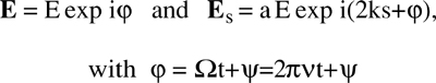
Amplitude E and phase φ of the oscillating field are assumed to be slowly varying quantities, and a balance is written of their time derivatives dE/dt and dφ/dt. Taking into account the external field re-entering the cavity after propagation to a remote target at distance s with field attenuation a, the Lamb’s equations are written as:

(4.36)

where:

a = At₁²η is the total field loss suffered by the reinjected field because of: (i) attenuation A in the go-and-return propagation to the target, (ii) double passage through the output mirror with a field transmission t₁, and (iii) mismatch η of the mode (cavity vs. returning) spatial distributions;

is the field transmission of the input mirror of field reflectance r₁ (explicitly, the power transmittance and reflection are T=t₁² and R=1-T=r₁²);

α=λ2(n₂-n₁)/8πτ₂₁Δτ_at is the active medium gain rate per unit length (of the field)

n₂-n₁ is the population inversion concentration (cm^-3);

Δν_at is the (atomic) gain line width and τ₂₁ is the active level lifetime;

β is the gain saturation coefficient;

Γ= Ω_c/2Q is the cavity field loss-rate (per unit time), including scattering in the medium and mirror transmission loss, explicitly Γ=t₁t₂c/2L+Γ_scc;

Ω_c is the cavity resonant frequency;

L is the cavity length, and c/2L is the longitudinal mode spacing;

ζ = (ν₀-ν_at)/Δν_at is the frequency detuning respect to the gain line center ν_at.

Letting (d/dt)E=0 in Eqs.4.36, we get the steady-state solution.

For the solitary laser (a=0), the quiescent values E₀, Ω₀ are readily found as and Ω=Ω₀=Ω_c+ζΓ/c.

For a≠0, we look for a small-perturbation solution of Eq.4.36, by letting E=E₀+ΔE and considering ΔE<<E₀ so that only first-order terms in ΔE are retained. By neglecting the pulling term ζ<<1 and dropping the unessential constant phase φ₀, after some algebra, we obtain the solution as:

(4.37a)

(4.37b)

where γ₀=α-Γ/c is the net gain per unit length available in the medium when oscillation is not yet started (it equals βE² because, in the permanent regime of oscillation, α+βE²-Γ/c=0).

Thus, at the first order of perturbation, the cavity field has an AM with modulation index m_A=(a/2Lγ₀) cos2ks proportional to the cosine of the external pathlength, and an FM with frequency deviation Δ/2π=a(c/4πL) sin2ks proportional to the sine of the external path-length.

Numerical example. The proportionality coefficient of AM is primarily the total attenuation a=Aηt₁², while the term 2Lγ₀ at the denominator has an order of magnitude not far away from unity in practical cases. Working on a diffusive target with a Gaussian beam with waist w₀, we find A=λ/πw₀ in the near field and A=w₀/s in the far field. For a retroreflector, it is A=1.

The mode superposition efficiency is η=1 for the diffuser and η²=2/[(w/w₀)²+(w₀/w)²] for the retroreflector, where w²=w₀²+(λ2s/πw₀)² is the spot size at distance 2s. In the far field, the product Aη is in both cases Aη∝1/s, for which we get an inverse-distance dependence of the signal level, which is typical of a coherent detection scheme (see [5], Ch.8) and well confirmed by experiments. Last, the output mirror (power) transmission is usually t₁²≈0.01 in a He-Ne laser. About the AM modulation index, α-Γ/c can be estimated from the amount of extra gain allowed for the startup of oscillation. In a He-Ne laser, usually α≈0.0005 cm^-1 and with L=20 cm, we have 2Lα≈0.02; with t₁²≈0.01, it would be Γ/c=t₁²/2L≈0.00025 cm^-1 and γ₀=0.00025 cm^-1.

To conclude our example, let us take a 20-cm He-Ne laser with a 0.2-mm waist w₀ and a 1-mr divergence. Working at s=500 mm distance on a diffuser target (far-field condition), we have: m_A=Aηt₁²/2Lγ₀≈ (0.2/500)0.01/0.00025 ·40=4 ·10^-4, while, on a retroreflector, it would be m_A≈0.2·0.01/0.01 =0.2. Correspondingly, the frequency deviation Δ/2π in the two cases is 750 MHz(0.2/500)0.01/6.28=500 Hz and 750MHz·0.2·0.01/6.28=250kHz, respectively.

Eqs.4.37a and 4.37b are an adequate description of the weak-injection regime (a<<1) in media with a population inversion n₂-n₁ only dependent on the pumping rate (α,β ≈ constant). These equations are well suited to He-Ne lasers and other media with small gain per unit length, for which they provide a good fit of theory to experimental data. They also hold at first approximation for semiconductor lasers at weak injection.

4.5.2.2 Bandwidth and noise of the injection interferometer

The frequency response of the interferometric signal (E, dφ/dt) to a variation of the distance s is made up by two contributions. One comes from the finite time that the laser medium takes to reach a new equilibrium condition established by the external distance, and the other is the delay associated with the propagation time of the field reflected by the target.

A third, usually dominant, limit is the frequency response of the photodetector translating the laser field into an electrical current signal. Because this limit is not inherent to the injection mechanism and can be separately evaluated, we will not deal with it furtherly.

To estimate the laser medium response time, we may take account that the cold laser cavity has a decay time τ_d=1/Γ. In addition, the laser oscillator is a feedback system with loop-gain G=1/2Lγ₀, as can be seen from Eq.4.37a where the effect of an input aE is transferred to an induced field aE/2Lγ₀. As a result of feedback theory, the resulting time constant of response is then τ=τ_d/G=2Lγ₀/Γ, and the corresponding bandwidth is B= 1/2πτ=Γ/4πLγ₀.

The external pathlength introduces a delay T=s/c in the effective field perturbing the cavity. Should the change in (E, dφ/dt) further interact with the laser cavity in the next round trip to the distance s, this delay would actually affect the frequency response. However, if the returned field in the first roundtrip is aE, it will become a²E in the second, and if a<<1, we may safely neglect this contribution, and state that the external distance effect is simply a delay T in response. This conclusion also applies to the medium-level of injection (Sect.4.5.2.3) that is applicable to semiconductor lasers.

With the usual values of parameters, B is in the range of some hundreds MHz in He-Ne lasers and of gigahertz (GHz) in semiconductor lasers.

To evaluate the noise, let us recall that the signal returned to the cavity is aE. If no amplification mechanism were present, the detected power would be a²E²=a²P. Because the detection is coherent, the quantum noise limit is attained. Thus, we may conclude that the minimum detectable displacement (or NED) of the injection interferometer is given by the diagram of Fig.4-18, in which we shall use a²P as the value of power, P being the power output from the unperturbed laser.

This result can be used as a default estimate of the injection interferometer noise. To improve the evaluation, however, we may account for the amplification undergone by the injected field. From Eqs.4.37, we can see that the laser supplies an AM signal 1/2Lγ₀ larger than the cosine component and a frequency FM signal equal to the sine component. In power, we have thus a gain G=1+(1/2Lγ₀)². From optical amplification theory (see [5], Sect.8.3) the noise figure is given by NF=1+2n_sp(G-1)/G, where n_sp=n₂/(n₂-n₁) is the inversion factor (≈1 for n₂>>n₁). Therefore, we may conclude that, at most, noise is increased by a modest 3 dB (or a factor 2) with respect to the a²P level when G>>1 and n_sp≈1.

4.5.2.3 The He-Ne injection interferometer

The experiment is carried out with a frequency-stabilized He-Ne laser (Appendix A1.2). In the practical implementation, we can use a Zeeman-split two-frequency source actuated by thermal expansion through a resistive wire wound on the He-Ne capillary tube, as originally reported in [10].

The two frequency split modes oscillate with linear, orthogonal polarized states. With a polarizer P placed in front of the main output mirror (Fig.4-23), one mode (say f₁) is selected for propagation to the remote target. The other mode (at f₂) is prevented from exiting the laser and is kept in cavity to act as a reference local oscillator for detection.

The propagated mode undergoes the AM and FM injection modulations and carries the optical path length 2ks information. When both modes are superposed on the photodetector placed on the rear mirror (Fig.4-23), they will beat and downconvert the AM and FM modulations to an electrical carrier at f₁-f₂.

Fig. 4-23 Injection interferometry with a He-Ne laser: two modes at slightly different frequencies (f₁-f₂≈100kHz) are generated by Zeeman-splitting due to a transversal magnetic field applied to the capillary tube. The two modes have linear orthogonal polarizations. One mode is allowed to propagate through the polarizer P, and the other mode is kept in the cavity. Polarizer P1 in front of the photodetector PH is oriented at 45° to allow beating of the propagated mode with the unperturbed mode kept in cavity. After frequency and amplitude demodulation, the signals sin 2ks and cos 2ks are obtained. The frequency signal is also used for frequency stabilization through the thermal actuator. Through differentiation and cross-multiplying of sin 2ks and cos 2ks, the v and s are recovered (from Ref.[10]).

The experimental waveforms of the photodetector current are shown in Fig.4-24. These are obtained with a 20-cm long tube, 0.5-mW commercial He-Ne laser aimed at a diffuser-surface target (a loudspeaker driven by a triangular waveform at audio frequency) placed at a s=40-cm distance. After AM and FM demodulation of the photodiode electrical signal, the waveforms of the interferometric signals S=sin 2ks and C=cos 2ks are obtained, as shown in Fig.4-25. Starting from these signals, several schemes can be devised to recover the displacement s.

Fig. 4-24 Waveforms of the electrical signal out from the photodiode when the target is a diffuser (white paper on a loudspeaker driven at audio frequency). To ease comparison, bottom traces with injection are shown along with top traces with the beam blocked off. On a 20 μs/div scale, the waveform reveals the FM signal in form of a time jitter; on a 1ms/div scale, the AM signal shows up in form of a ripple. Using a corner cube target, the signals become much larger and require an attenuation inserted on the beam (from Ref.[10]).

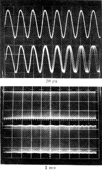
Fig. 4-25 Top: waveforms of target driving signal and of the interferometric signals S=sin 2ks and C=cos 2ks demodulated from the photodiode output; bottom: the reconstructed velocity signal v=ds/dt and its integral, the displacement s. Time scale: 1ms/div (from Ref.[10]).

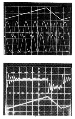
For example, we can acquire S and C through an A/D interface and use a small dedicated computer to calculate s. For small displacements Δs<λ/2, Δs is simply computed as Δs =(1/2k) atan S/C.

For large displacements, because atan is a multivalued function, we shall compute s looking at the evolution of Δs. Using a digital processing, we may add to (1/2k) atanS/C an increment ±λ/4 for each zero-crossing of C, with the sign (+) for U=1 and (−) for U=0, where U is given by Eq.4.6.

Alternatively, we may prefer to use a straightforward analogue processing performed by a few electronic analogue circuit blocks. Taking the time derivatives of S and C, we get:

where v=ds/dt is the velocity. By cross-multiplying the two derivatives to C and S and subtracting, we have:

(4.39)

and, with a time integration, we obtain the displacement s = ∫ v dt [10].

The circuit performing this analog processing is shown in Fig.4-23. With this circuit, the reconstructed velocity and displacement for a triangular waveform excitation of the target are those reported in Fig.4-25. Note that the s(t) and v(t) waveforms deviate somehow from those expected from the drive waveform. However, this is simply a consequence of the loudspeaker real response and is actually a measurement of the response itself.

Here, the target was a piece of plain white paper glued on the loudspeaker. Accordingly, the back-scattered field received by the laser obeys the speckle-pattern statistics. The dynamic range is then limited by the longitudinal speckle dimension S₁ = λs²/w² (where w is the spot size on the target and s is the target-laser distance). A peculiar feature of the injection interferometer is the ability to self-filter the returned field spatially.

The transversal speckle size is S_t = λs/w, and the far-field spot size is w=(λ/w₀)s. By substitution, we get S_t=w₀, that is, the returning speckle (or coherence) size S_t exactly matches the laser mode size w₀, and no waste of power occurs.

Another field of application is the pickup of biological motility signals, like respiratory sounds and blood pulsation [16]. In Fig.4-26, we can see the experimental trace of the blood pulsation detected on a finger, revealing the cardiac pulsation, detected remotely without contact with the tissues under measurement.

Fig. 4-26 Pickup of biological motility with the He-Ne laser injection interferometer. The blood pulsation waveform is measured on a finger and reveals the left ventricular ejection (LVE) as well as the dicrotic incisure (DI). The vertical scale is 0.1 μm/div, and the horizontal scale is 0.2 s/div.

Of course, the injection interferometer of Fig.4-23 can operate on a corner cube target as well [17]. In this case, the returned signal is much larger than with the diffusing target, and an optical attenuator is inserted on the beam to avoid high-level injection effects. When counts are drawn out of signals C and S, the performance is much the same as the two-frequency interferometer.

The He-Ne laser is well suited for the weak-level injection interferometer, because it readily provides two frequency-split modes, one for propagation and the other for internal reference and down-conversion to electrical frequency. However, because the He-Ne is rather bulky and its reliability is questionable, we may think of replacing it with a semiconductor laser.

In diode lasers, unfortunately, we are not able to make the equivalent of a Zeeman dual-frequency oscillation. Thus, just the AM signal is available as a modulation in emitted power, whereas the FM signal cannot be recovered. This brings about the ambiguity of the cos 2ks function, which is not easily circumvented for the application to displacement measurements, at least in the weak-injection regime. On the other hand, the single interferometric AM signal cos 2ks is sufficient for small-vibration measurements, when amplitude Δs is less than or comparable to λ/2 (Sect.4.6).

4.5.2.4 Analysis of injection at medium-feedback level

The regime of injection at moderate levels of a back-reflected field is important in applications because it permits collecting, with a single AM signal, the same information supplied by the signal-pair cos 2ks and sin 2ks. In this regime, we can perform an unambiguous measurement of displacement, in increments of a fraction of wavelength with the correct sign (e.g., + for increasing distance, - for decreasing), yet with a single signal.

Experimentally, we have the setup of Fig. 4-27, in which a laser (usually, a semiconductor single-mode laser) is aimed through a collimating objective lens to a mirror target. A variable attenuator is used for adjusting the level of power returned into the laser cavity. Detection can be performed by a photodiode placed everywhere on the beam (because the AM signal is carried by the beam itself, a distinctive feature compared to conventional interferometers. Most conveniently, however, we may use the monitor PD usually incorporated in the diode-laser package at the rear mirror of the laser.

Fig. 4-27 Conceptual arrangement for experiments with an injection interferometer: using a variable optical attenuator, we adjust the level of injection and look at the AM waveform using the rear-mirror photodiode PD.

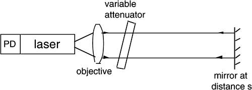
Fig. 4-28 Waveforms of optical power in an injection interferometer. At weak levels of injection (C<<1), the normal dependence cos2ks from external phase shift is found. Increasing the injection, the waveform becomes progressively distorted and asymmetric. As C reaches unity, a switching occurs with period 2π. If the target reverses its motion, the phase shift decreases, and the waveform becomes time-inverted, except at the switching point where now it follows the up arrow. Beyond C≥4.6, more than one switching per period occurs, and operation becomes affected by errors.

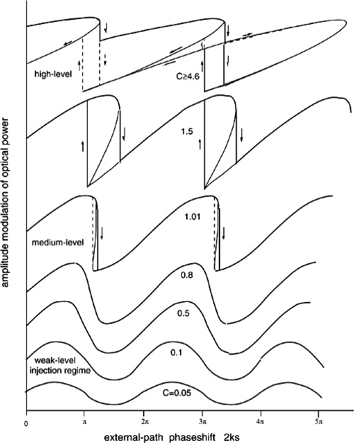
Thus, a signal I=σP is obtained, which is proportional to the power P emitted by the laser and that carries the AM modulation waveform, that is, cos2ks at low-injection level.

We enter the moderate or medium level of injection when, at increasing back-reflected power, the interferometric signal cos 2ks becomes appreciably distorted (Fig.4-28). First, the waveform exhibits a leading semiperiod slower than the trailing semiperiod. Then, when injection is increased further and C (Eq.4.35) reaches unity, the waveform becomes sawtooth like, with a sharp switching in amplitude. Then, we find one switching per period of the optical path length 2ks, that is, one for each Δs=λ/2 increment of displacement and, important to note, the switching is negative-going when 2ks is increasing (Fig.4-28).

Now, if the motion of the target is reversed, the diagram of Fig.4-28 still applies, but with 2ks runs from right to left. The waveform has now a leading semiperiod faster than the trailing semiperiod and, most important, the switching is now positive-going (and occurs at a slightly changed value of 2ks because of hysteresis).

The strategy to make a displacement measurement without ambiguity easily follows. By operating the injection interferometer at C>1, we count each switching corresponding to λ/2. Counts are with the positive sign if the transition is up-going and with the negative sign if it is down-going. Operation is limited to the range 1<C<4.6 where there is just one switching per period (Fig.4-28) [15]. The experiment will be developed in more detail in next section. In the basic setup of Fig.4-27, the FM signal cannot be detected. However, we should expect that the sin2ks signal, similar to the cos2ks, is asymmetrical and has switching on its period [15].

4.5.2.5 Analysis by the three-mirror model

Let us consider the injection interferometer as a three-mirror cavity laser, as shown in Fig.4-29. Analyzing the round trip loop, we can write the field returning to the initial point as the sum of two contributions, from the paths internal and external to the laser cavity, as:

(4.40)

where r₁ and r₂ are the mirrors’ field reflectivity, α^*=α-βE²-Γ/c is the net gain (or, gain less loss) per unit length, L is the laser cavity length, and a=A(1-r₁²)η is total field loss in the external propagation to the third mirror. Thus, the loop gain is:

(4.41)

Because of the well-known Barkhausen criterion of oscillators, G_loop shall be exactly unity in the permanent regime of oscillation, and phase φ_loop exactly zero, or:

(4.42)

Fig. 4-29 Schematization of the injection interferometer as a three-mirror laser

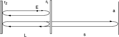
When a=0, Eq.4.42 requires (net gain equal to mirror losses) and φ_loop=2kL=0_[mod2π] (cavity resonance condition), or that 2ks is an integer multiple of 2π. Writing the condition as 2·2πn₁Lν₀/c=N2π the unperturbed frequency is found as ν₀=Nc/2n₁L, with N being the order of the mode and n₁ the index of refraction of the active medium. Near to resonance, if the actual frequency ν deviates from ν₀, the part of 2kL in excess of 2π can be expressed as 2kL=4πn₁L(ν-ν₀/c [as 4πn₁Lν₀/c=N2π].

In presence of feedback (a≠0), the phase condition is φ_loop=atan[ImG_loop/ReG_loop]=0 or, more simply, Im{G_loop}=0, and explicitly reads:

(4.43)

Using r₁r₂ exp 2α^*L=1 in Eq.4.43, assuming in the first term that ν-ν₀ is small (so that sin x ≈ x) and noting that 2ks=4πsν/c≈4πsν₀/c, we obtain:

(4.44)

This equation tells us that, in presence of injection, the actual frequency ν deviates from the frequency ν₀ of the solitary laser by an amount (c/4πLn₁) a sin2ks, which is easily recognized to coincide with the factor Δ that is derived by Lamb’s equations (Eq.4.37) treatment for small a.

Now, if we plot ν versus ν₀ as given by Eq.4.44, we get a sinusoid curve superposed to a straight line (Fig.4-30). When the distance s is changed by λ/2, the argument of the sine changes by 2π, and ν covers the full swing of the sine curve displayed in Fig.4-30. Thus, the actual frequency obtained depends on the residue Δs of distance s= Nλ/2+Δs to the nearest integer multiple of λ/2. We can draw a horizontal line (the dotted line in Fig.4-30) to represent the working point determined by Δs, which moves vertically along a full period of the sinusoid as Δs varies of λ/2.

As long as the amplitude of the sinusoid is minute, only one intersection is found, and we are in the case of weak-feedback injection. However, at increased injection, we may have a curve with three intersections to a horizontal line. The frequency then stops following the sine curve smoothly and will flip suddenly to another portion of the curve (Fig.4-30).

We may take the boundary from the weak- to the moderate-feedback regime as that of the curve with a horizontal flex. Mathematically, the condition of a horizontal flex in the y-x diagram, for a function y=x+A sin Bx is AB=1. Comparing with Eq.4.44, we find the condition (c/4πLn₁)a4πs/c=1, or also: as/Ln₁=1.

We may now define a factor describing the strength of injection as C= as/Ln₁ and state that, for C>1, we enter in the regime of frequency switching. This factor coincides with that already quoted in Eq.4.35, except for the term specific of the semiconductor lasers.

Fig. 4-30 Frequency of the injection-perturbed oscillation ν as a function of the solitary laser frequency ν₀. At increasing feedback level (C values), the curve has three intersects with the dotted line representing the distance s and exhibits switching.

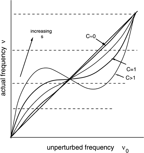
About the AM amplitude signal, from the amplitude Barkhausen criterion, it is . Letting E=E₀+ΔE in Eq.4.41, developing the mosulus and considering ΔE<<E₀ in it, after some lengthy calculation we find:

(4.45)

This expression is coincident with the weak-feedback result (Eq.4.37a) for a<<1. Moreover, when the factor a increases, the waveform becomes distorted because of the cosine dependence at the denominator. At C=1, when frequency switches, ΔE and the AM signal will, too, because of the ν-dependence of the cosine term at the numerator.

By solving numerically Eq.4.44 (or using the diagram of Fig.4-30), we can find a function ν=F(4πsν₀/c) that replaces ν in sin4πsν/c at the moderate feedback level.

Using ν=F(s) in Eq.4.45, the diagram of Fig.4-28 can be obtained.

As a conclusion of the previous analysis, by applying the Barkhausen’s criteria to the three-mirror cavity model [15,18,22], we have been able to derive the basic results describing the moderate-level feedback regime. In particular, switching of frequency and amplitude signals are found to occur at a critical value C≥1. Using them, we are able to perform an unambiguous measurement of displacement using the amplitude waveform only.

4.5.2.6 Analysis by the Lang and Kobayashi equations

A more rigorous treatment of moderate-level feedback, including the effects specific to a semiconductor laser, is provided by the description through the Lang and Kobayashi equations [13,14]. These equations rephrase Lamb’s equations for amplitude E and phase φ in a perhaps more detailed way, and also add a third equation for the active-level population and its dependence from pumping rate and cavity field. In presence of feedback, the Lang and Kobayashi equations read [14,15]:

(4.46a)

(4.46b)

(4.46c)

where: g_N is the gain coefficient [typically 8·10^-7cm³s^-1]; in terms of the Lamb’s coefficient

α, (Eq.4.36) it is g_N =αc/(n₂-n₁)=λ²c/8πτ₂₁Δν_at.

N=N(t) is the carrier (electron-hole pairs) density (cm^-3) in the active region.

N_tr and N_T are the carrier density (cm^-3) at transparency and at threshold of the solitary laser [typically a few 10¹⁸cm^-3], and it is g_N(N_T-N_tr) =1/τ_p.

τ_p is the photon lifetime [typically a few ps] related to absorption and mirror losses a = At₁²η is the total field loss suffered by the reinjected field in the roundtrip path.

L is the laser cavity length, and n₁ is the active-medium index of refraction.

τ =2s/c is the external roundtrip time

ω₀ is the (angular) frequency of the unperturbed laser.

α_en is the linewidth enhancement factor [13] [typically 3 to 6 in diode lasers].

J is the pump current density (A/cm^-2, d =active layer thickness

τ_s is the charge-carrier lifetime [typically a few ns].

The analysis of the moderate-level injection [15] starts with letting dE(t)/dt=0 and (d/dt)N =0 in Eqs.4.46a and 4.46c, and solving for the stationary values E_0f and N_0f in presence of feedback. From Eq.4.46a we get:

(4.47)

The term on the right-hand side shows that feedback induces a modulation of the carrier density N. As a consequence, a variation of voltage developed across the laser-diode junction is induced [15, 21]. This is a signal that can indeed be recovered and used as the interferometer output in place of the normal photodiode output.

By inserting Eq.4.47 in Eq.4.46b, we find the perturbed oscillation frequency ω_0f as:

(4.48)

This equation can be brought to coincide with the Barkhausen phase-condition (Eq.4.44). Now, we can use the feedback parameter C, already defined by Eq.4.35 and repeated here for convenience:

By multiplying both members of Eq.4.48 by τ=2s/c, it becomes:

(4.49)

or also, using an identity of trigonometry:

(4.50)

In a 2π-period of ω₀τ, Eq.4.50 has just one solution for C<1 (weak-level injection), and three solutions for 1<C<4.6 (moderate-level injection). One solution is unstable, however, and implies a switching between the other two states, the stable solutions. Last, for C>4.6, multiple switching is found in a single 2π-period of ω_0fτ (strong-level injection). From Eq.4.46c, letting (d/dt)N=0, the electric field with feedback E_0f² is:

(4.51)

whereas, from Eqs.4.46a and 4.46c, with no feedback, we have the quiescent point E₀²=τ_pg_N(N₀-N_tr)=τ_p(J/ed-N₀/τ_s), and P₀∝ E₀².

Using this result and N_0f as given by Eq.4.47, we obtain, after some algebra, the optical power variation ΔP ∝ E_0f²-E₀² induced by feedback as:

(4.52)

which is similar to Eq.4.45 and becomes the familiar ΔP₀m_Acos2ks expression for a<<1.

A last result worth mentioning about the moderate-level injection [15,22] is the reconstruction of the displacement waveform s(t) from the AM interferometric signal given by Eq.4.52. By combining Eqs.4.50 and 4.52, we can obtain the following expression relating ω_0fτ=2ks to the instantaneous ΔP/ΔP₀=F(t) modulation:

(4.53)

where the sign shall be taken ‘+’ for dF(t)/dt×(ds/dt) <0, and ‘-’ for dF(t)/dt×(ds/dt) >0, and m shall be increased by 1 every two zero-crossings of F(t) [15,22].

4.5.2.7 The laser-diode injection interferometer

Starting from the basic setup of Fig.4-27, a number of researchers [11,15,18-27] have reported about the development of laser-diode injection interferometers for measurements of displacements, velocity and for the detection of remote targets. The typical waveforms of the current detected under moderate feedback conditions with single-mode laser diodes emitting either in the visible (λ=680 nm) or in the near infrared (λ=800 nm) are shown in Fig.4-31.

Fig. 4-31 Injection interferometry experimental signals, in response to sinusoidal drive s(t) signal (top trace in both pictures). Top picture: at C=0.6, the cos 2ks waveform is slightly distorted, with falling semiperiods somewhat faster than the rising ones; at C larger than 1, a switching occurs in the fall semiperiod (bottom picture is for C=2.2). Wavelength: λ=850 nm. Time scale: 2 ms/div. (from Ref.[15], by courtesy of IEEE).

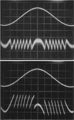
Fig. 4-32 Drive s(t) (uppermost) and theoretical ΔP/P waveforms corresponding to the experimental data of Fig.4-31, for a few values of the feedback parameter C, ranging from weak to moderate level of injection (C=0.01, 0.7, and 3.3 from top to bottom). The relative vertical scale of ΔP/ P signal is 0.5, 3, and 10 (top to bottom). Horizontal scale: 1ms/div.

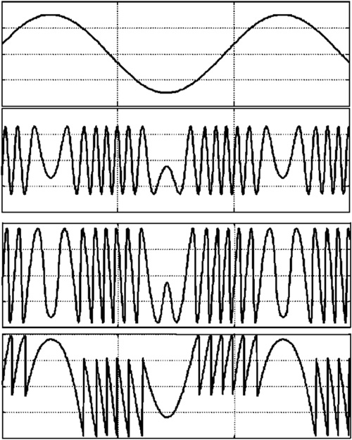
Experimental results nicely match the analytical expressions found in the previous section, as exemplified by the curves reported in Fig.4-32 for a few values of C comparable with those of Fig.4-31.

The block scheme of a displacement interferometer working on λ/2-step counting is shown in Fig.4-33. The target is aimed through a collimating objective lens (typically a 5-mm focal length) or by a telescope (with typical ×20 magnification). An optical attenuator is inserted in the target path to adjust the feedback parameter to be in the range 1<C<4.6, the desired regime of a single switching per period.

The signal out from photodiode (in most practical schemes, the monitor photodiode of the laser chip is adequate for use) is passed to a transimpedance preamplifier and then to a differentiator with a short time constant τ_d=RC. Out of the differentiator, the up/down switchings are a sequence of positive/negative short (≈τ_d) pulses. We can easily separate the pulses in two channels, rectify the negative ones, and send one channel to the up-count input of a counter, and the other to the down-count input. Last, multiplying by the scale factor λ/2 brings the readout of the display to decimal metric units.

Fig. 4-33 Block scheme of the laser-diode injection interferometer working on the waveform switching to count displacement in steps of λ/2

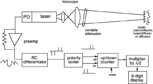
Thus, with a minimum part count, we are able to build an interferometer measuring target displacement in steps of λ/2, or 425-nm per least-significant digit (at λ= 850-nm).

As in all interferometers, the maximum distance that can be covered in the displacement measurement is limited by the coherence length of the laser diode. This can be up to a several meters in selected narrow-line plain (Fabry-Perot) lasers.

The target for the measurement may be a corner cube, to allow for a sizeable attenuation, or a Scotchlite tape or varnish. This provides a gain ≈40 with respect to the normal Lambertian diffuser. Also, we may use a simple plain diffuser, that is, white paper or the like. In all cases, we shall keep the signal in the single switching (1<C<4.6) regime. This requires a careful design of the objective optics when using the plain diffuser because the signal from it is barely sufficient. With the corner cube or the superdiffuser, the signal is even too large, and we shall adjust it by the variable attenuator, eventually changing its setting with the working distance. It may then be advisable to add a servo-loop control of the attenuation to get a self-adjusting operation.

A strategy to stabilize the signal amplitude in the 1<C<4.6 range is the following. Superposed to the dc laser diode current, we add a small modulation signal i(t) at audio frequency. The emitted wavelength then varies as Δλ(t)=α_I Δi(t), where α_I is the current coefficient (see App.A1.3.1). We choose 2Δks=4πsΔλ/λ²≥2π so that at least one switching occurs in a period of modulation, even for a target at rest. Then, we look at the differentiated signal and, if it is missing, we decrease the optical attenuation until the signal shows up and allow for a moderate (e.g., x2) overdrive. To have a simple and cheap controlled-voltage attenuator, we can use a Liquid Crystal (LC) sandwiched between two polarizers. The birefringence of the LC is controlled by the applied voltage, resulting in an adjustable attenuation. The up and down switching of the modulation has a zero-mean value and does not interfere with the displacement measurement.

About precision, the laser-diode interferometer is different from the He-Ne laser because it does not possess an inherent calibration of wavelength. In a Fabry-Perot semiconductor laser, wavelength is markedly dependent on drive current and temperature, mode-hopping can occur, and the actual λ=λ(I,T) curve is also dependent on the previous story of I,T changes. In the most common and cheaper Fabry-Perot cavity lasers, the typical temperature and current coefficients are dλ/λdT=2-5 10^-6(°C^-1) and dλ/λdI=1-3 10^-6(mA^-1) (see also App.A1.3.1).

Thus, we may expect an error in the displacement measurement of several ppm for a 1-°C or a 1-mA variation of chip temperature or diode drive current.

The situation is much better in DFB or DBR lasers, where the incorporation of a grating reflector alleviates the temperature dependence and nearly eliminates the current dependence. However, these lasers are not easily available so far for wavelengths other than the fiber third-window (λ≈1500 nm) and are much more expensive than Fabry-Perot types.

Altogether, the previous points call for a thermal stabilization of the laser chip (with a TEC or Peltier cell module) and of the drive current (by a regulated and low-ripple supply). With Fabry-Perot lasers, using a stabilization of 0.01 °C in temperature and ±10 μA in current, the instrumental accuracy of the injection interferometer has been evaluated to be ±1 count (≈0.4μm) at 50 cm distance, or ±1 ppm [15]. In addition, DFB lasers with a long-term stability of Δλ/λ=0.1 ppm have been reported in the laboratory [28].

To extend the operation of the interferometer to sub-λ resolution, the photodetected signals can be acquired by a computer, and the calculation of 2ks is then performed with the aid of Eq.4.53. This scheme of analogue processing has been shown [10,22] to be able to reconstruct the displacement waveform s(t) with a ±5nm accuracy, with no constraint imposed on the signal s(t) waveform.

In conclusion, the advantages and disadvantages of the laser-diode injection interferometer, as compared to conventional types, can be summarized as follows:

– It has a minimum optical part-count (no external optical interferometer) and relatively simple electronics.

– The optical head (laser, lens, attenuator) is very compact with a distinct advantage for ease of mounting in experiments short of space.

– No critical alignment on the target is required.

– No spatial, wavelength or stray-light filtering are necessary; the laser cavity itself provides these functions.

– Operation on a normal diffusing target surface is readily achieved, without modifications of the setup.

– The interferometric signal can be detected everywhere on the beam, and also from the target side.

– λ/2 resolution with digital processing and sub-λ sensitivity with analogue are easily achieved up to several hundreds kHz or MHz bandwidth.

– Performances are comparable to those of conventional interferometers.

– Wavelength accuracy and long-term stability may be of concern.

– Flexibility of reconfiguration is modest.

4.6 Laser Vibrometry

A laser vibrometer is an interferometer especially designed for use as an instrument capable of detecting and measuring small vibrations in a variety of applications related to mechanical, automotive, avionics, and construction engineering, as well as in biological structures. Usually, vibration means a periodic displacement waveform, with typical amplitudes of interest ranging from less than 1 nm to tens of μm, and frequency ranging from less than 0.1 Hz to perhaps 1 MHz.

Vibrometry is an important diagnostic tool and is commonly used to measure vibrations of a structure under test or to determine its frequency response to a periodic excitation applied externally. Both modes of operations allow collecting important information about the structure for design, verification, and testing purposes. With respect to other measurement techniques based on electronic sensors, the laser vibrometer has the key advantage of noncontact operation and does not disturb the structure under test.

The best configuration of the vibrometer is different according to the allowed or required distance of operation of it from the target under test. In the following sections, we describe vibrometers aimed to a performance optimized on three ranges of interest: (i) short distance (say less than 10 cm), (ii) medium distance (a fraction to several meters), and (iii) long distance (up to hundreds meters).

Basically, we may also use a displacement interferometer as a vibrometer (Sect.4.2.3.4), but three specific features shall be considered for design optimization.

First, superposed to the small displacement, we may find a relatively large (up to hundreds of μm) ambient-induced microphonics disturbance. This can be strongly reduced if we are permitted to work on an antivibration laboratory table, but cannot be avoided if we aim to inthe-field operation of our instrument. Second, we are forbidden to use anything that disturbs the target and its vibration state, like a corner cube, and the vibrometer is to work directly on the natural target surface, normally a gray (δ<1) diffuser. Thus, the returned field is much attenuated and subjected to the speckle-pattern statistics (Sect.4.4.7 and Ch.5). Last, the range of displacement to be measured is very small and it may permit relaxing the coherence length needed when operation is on short distance, or when we can balance the interferometer arm path lengths.

4.6.1 Short-Distance Vibrometry

Early experiments in short-distance interferometric vibrometry were developed in the 1970s around a Michelson configuration, which was modified by adding lenses focusing the reference and measurement beams and by adding a provision for dynamical tracking of the reference path to compensate for the microphonics-induced ambient disturbances (Fig.4-34). This is accomplished by the piezo actuator in the reference path, which is either a diffuser (as shown in Fig.4-34) or a reflective surface. Light scattered by the diffusing target in the measurement arm is collected back by the lens and recombined on the photodetector.

The photodetected signal, I_ph=I₀[1+cos2k(s_m-s_r)], is preamplified by the front-end giving a signal V_ph=RI₀[1+cos2k(s_m-s_r)] and is low-pass filtered with corner frequency f₁. A constant voltage V_ref is then subtracted from V_ph, and the result, amplified by A, constitutes the error-signal supplied to the piezo.

Because of the feedback loop, the system adjusts itself at a quiescent point where the error signal is nearly zero, or V_ph-V_ref≈0. Setting V_ref=RI₀, we get the condition 0=V_ph-RI₀ = RI₀cos2k(s_m-s_r). For s_m very small, the quiescent point is 2ks_r = π/2, and we get:

(4.54)

The best choice for the low-pass frequency f₁ depends on the actual level and frequency content of the disturbance coming from the ambient. In most cases, the disturbance spectrum is found to damp off quickly between, say f_dist= 100-1000 Hz.

Choosing f₁≈ f_dist, the low frequency components (f< f₁) are suppressed because of the feedback effect. Instead, signals s_m(t) with frequency content f>f₁ find the loop ineffective (interrupted by the filter) and are passed on to the output. From a well-known result of feedback theory, the actual suppression factor is given by the loop-gain G.

By inspection of Fig.4-34, the dc loop gain is easily found as G₀=R I₀Aκ, where κ=Δs/V (μm/Volt) is the conversion factor of the piezo. We can readily make G₀=10³ and nearly eliminate the disturbance. In frequency, the loop gain is G(f)= G₀/[1+(f/f₁)²]^n/2, where n is the order of the filter (n=1 for a simple RC). Signals with f>f₁ find a small G(f) and are not reduced, so we can take them either from the transimpedance output or from the filter high-pass output as indicated in Fig.4-34.

Of course, signals with frequency content f<f₁ are suppressed, like the disturbances. To minimize loss of useful spectrum, we will make the filter frequency f₁ adjustable and trim it to optimize the outcome of the measurement by inspecting the result.

The speckle-pattern regime of operation is of little problem for the vibrometer. Should eventually the reference or measurement fields fall on a dark (weak amplitude) speckle, it will suffice to move the target surface transversally just a little bit (by a few μm) to find another, bright high-amplitude speckle.

The same result can be obtained by a fine position adjustment of the lenses, too.

Regarding the phase error generated by the speckle-pattern statistics (Sect.4.4.7), the re-radiated field received through the lens is in the far-field of the target [large S₁ in Eq.(4.31)] and generates a negligible error, whereas changes in the spot projected on the target due to longitudinal or transversal displacements may be of concern.

The longitudinal displacement introduces a negligible error as far as the amplitude of vibration (signal plus disturbance) is small as compared to the depth of focus of the lens Δf. This is given by Δf =λ/πNA², where NA is the lens numerical aperture and typically is Δf≈ 0.1-1 mm.

On the other hand, transversal displacements of the target are to be more tightly controlled. They are required to be small with respect to the focused spot size Δw=λ/πNA (Ref.[5], App.A2), which may have a typical value of ≈5 to 30 μm.

Thus, it may be important to align the specimen under test to get the vibration to be parallel to the impinging beam axis.

In addition to the mechanical segment, a short-distance vibrometer is useful for noncon-tact measurements of otherwise undetectable minute vibrations in a variety of devices, including electronic and piezoelectric components. As an illustration, we report in Fig.4-35 the measurement of sub-nm amplitude waves in a Surface Acoustic-Wave (SAW) filter, obtained with a setup similar to that reported in Fig.4-34. The result has pointed out the difference between the Stoneley regime and the normal SAW regime [29] of surface waves.

Fig. 4-34 A short-distance vibrometer for measurements on small size specimen. The reference beam is focused on the diffuser surface driven by a piezo actuator. The interferometric signal is low-pass filtered, amplified, and sent to the piezo. Because of the feedback loop, the working point is locked to I_ph=V_ref/R, the half-fringe point of the interferometric signal I_ph=I₀[1+cos2k(s_m-s_r)]. The vibration signal, at f>f₁, is taken out from the high-pass output V_out of the filter as RI₀2ks_m.

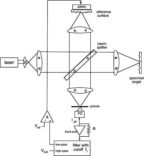
To evaluate the ultimate sensitivity (or NED) of the vibrometer, we may start considering that the optical power P₀ supplied by the laser is sent half to the measurement and half to the reference path. All this power reaches the target, but, in the rediffusion process, only a fraction η of it is sent back into a single spatial mode for coherent superposition at the photodetector.

If w₁ is the spot size of the Gaussian beam and =λ/πw₁ is the associated diffraction angle, the power fraction is η=(λ/πw₁)². With typical values for a He-Ne laser, P₀=1mW, λ=0.633 μm and w₁ =0.5 mm, we have η=1.6 10^-7. The useful power is then ηP₀/2=0.8 10-¹⁰ W, and, from the diagram of Fig.4-18, we can find the minimum measurable amplitude of vibration as NED=(0.6 10^-6m) , where B is the bandwidth of the measurement in Hz.

This very appealing result is to be regarded as a conservative estimate. Indeed, a real target is not an ideal diffuser, but may even have a minor (e.g.<0.1%) residual specular reflection. The reflection helps because it makes the statistics more regular. This will readily overwhelm the very small η and make the signal increase even of a few order of magnitude.

Fig. 4-35 Detection of sub-nm (1Å=0.1 nm) vibrations in a SAW device. Bulk Stoneley waves and ordinary surface waves are discriminated by their amplitude. Central frequency of the SAW is 8 MHz (from Ref.[29], by courtesy of the American Physical Society).

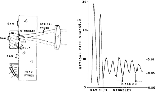
With regard to the spatial resolution of the vibration measurement, this is given by the spot size Δw projected by the lens on the target in the focal plane.

In general we have (Eq.A.2.10, Ref.[5]) Δw=λ/πNA, where NA=arcsin D/2F is the numerical aperture of the lens. However, if the lens diameter D is not filled completely by the beam, NA is determined by the spot size radius as NA= arcsin Δw/F.

Using λ=0.633 μm, w₁ =0.5 mm, and F=20 mm, we obtain a spot size Δw=16 μm. This figure represents the elemental pixel of spatial resolution.

Last, the bandwidth of response of the vibrometer is primarily determined by the high frequency cutoff of the photodiode transimpedance amplifier and associated electronic processing circuits. With an available optical power in the ηP₀≈100 pW range (or, I_ph≈100 pA), we may use a 10 to 100kΩ feedback resistance and get, from state-of-the-art design (see Sect.3.5, Ref.[5]), bandwidth of 1 to 10 MHz.

In conclusion, the approach described previously is a good technical choice to develop a short-distance vibrometer with nm-sensitivity, ≈20 μm sampling size, and MHz bandwidth.

We can classify this vibrometer as homodyne with low-frequency half-fringe stabilization as compared to other types described in the following sections. Homodyne is because the reference and measurement beams share the same frequency, half-fringe stabilization is because we work at the midpoint of the sine-signal dynamic range and, by doing that with a feedback loop, we get rid of slow undesired low-frequency microphonics induced by the external ambient.

4.6.1.1 High-frequency fringe tracking

Another approach, evolved from the basic scheme of Fig.4-34, is that of homodyne with high-frequency fringe tracking. If we remove the low-pass filter in Fig.4-34 and use a small, high frequency piezo (or any other path-length actuator) with say, a f_p≈1 MHz pass-band, we are able to lock the interferometric signal always at half-fringe, irrespective of the signal spectrum, up to f_p.

Because the error signal is always null-balanced, or RI₀ sin2k(s_m-s_r)≈0, the photocurrent I_ph shows no appreciable signal. However, because it is also s_m-s_r≈0, the reference s_r tracks the measurement displacement s_m. Thus, if the piezo response is linear, its drive voltage V_dr=Δs_r/κ is just proportional to the desired signal s_m to be measured.

One advantage of the high-frequency tracking is the much increased dynamic range and improved linearity. Because the working point is always at half fringe, the responsivity R= Δs_m/V_dr is a constant at a value found from V_dr= ARI₀sin2k(s_m-s_r) as R= 1/(ARI₀2k).

This is true even for a large (>>λ/2) amplitude of vibration, which suffer from the nonlinearity of the sine function in the low-pass scheme. Also the dynamic range is increased to a value G₀λ/2, because of feedback, and can easily attain several hundred micrometers.

On the other hand, a drawback of the high-frequency scheme is that spurious ambient-related disturbances are not eliminated, and we need to look for an alternative strategy to get rid of them.

As the superposed disturbance is physically undistinguishable from the signal, we need supplementary information about it to succeed. One is about the spectral content of the signal. If we look to signals with frequency well in excess of the typical disturbance frequency (f_dist < ≈100Hz), we can obviously simply filter out the disturbance from the output V_dr signal. Second and less demanding, frequently it happens that the experiment allows us to switch on and off the signal, and the perturbation is statistically well behaved and stationary (that is, has an average power spectrum stable in time).

Then, we may take advantage of the linear regime of response. Because of this, the output V_dr=V_m+V_arv is the sum of the effects separately produced by measurement s_m and ambient-related disturbance s_arv. We cannot hope the disturbance will replicate itself in different runs, i.e., computing the signal as V_m=V_dr-V_arv is not acceptable, whereas the corresponding power spectrum S_arv(ω) is much likely to be constant, at least in a short period of measurement time. Therefore, we acquire the signal V_m during two equal time slots, one with signal on and one with the signal off and compute its power spectrum (e.g., by a FFT routine). The corresponding power spectra are S_dr1= S_m+S_arv and S_dr2=S_arv. By subtraction, S_dr1-S_dr2=S_m is the required signal power spectrum that is obtained.

The price for such a power-spectrum subtraction scheme is that the phase relationship of different frequency components in the signal is lost because the power spectrum is the square modulus of the Fourier transform of the s(t) signal in the time domain.

Instead of a high-frequency feedback loop, we may also think of a quasi-dc, very-low frequency compensation of the reference path, again looking at the photocurrent half-fringe. This is easily implemented with nearly any kind of actuator (motorized micropositioning stage, loudspeaker cone, or even a manual control) and has been experimented with since the early time of vibrometry. Of course, we don’t have, in this case, any benefit from the loop-gain on the dynamic range (s_m-s_r is limited to λ/2) nor on linearity (the straight sin2ks dependence applies). However, the fringe tracking avoids fringe hopping and the related erratic functioning of the vibrometer, and we can again apply the spectrum subtraction scheme, though with a much more limited performance.

4.6.2 Medium-Distance Vibrometry

In the range of medium distances (a fraction to several meters) the concept of injection interferometry is readily applied to develop a homodyne, high-frequency fringe-stabilized vibrometer with high performances.

4.6.2.1 An Injection Vibrometer, fringe stabilized

As it will be clear in the following, the best choice is to operate at the medium-level of injection (Sect.4.5.2.3), that is, with 1<C<4.6.

Because we have C≈as/L from Eq.4-35, the desired level C≈1 requires a distance s≈L/a. Recalling the result of the efficiency calculation in last section, , we may have typically a≈4 10^-4. For a normal L≈200-μm diode-laser cavity, this requires a distance s≈0.2mm/ 4 10^-4= 50 cm, which is a value classified as medium-distance range (s≈0.3…3 m) of operation. This range is still covered by the coherence length of plain Fabry-Perot laser diodes, the ideal choice for low cost and simple set-up.

In the medium-level injection regime, the photocurrent I_ph is a distorted sine wave response resembling a saw-tooth waveform (Figs.4-28 and 4-31 or 4-32). We will use the quasilinear ramp semiperiod for operation.

Thus, linearity of response (before feedback is applied) is improved with the additional advantage of expanding the dynamic range of control.

The injection interferometer does not have a reference path, and this may appear a serious hindrance. However, we can take advantage of the wavelength dependence λ=λ(I_dc) from the laser drive current to adjust 2ks exactly to π/2. As shown in the schematic of Fig.4-36, we look at the interferometric signal from the front-end preamplifier, V_ph=RI₀(1+cos 2ks), and subtract the half fringe dc term V_ph0=RI₀. The loop ends up driving the laser current, with the error signal superposed to the fixed dc level I_dc =V_bias/R_c chosen to set the laser power.

To lock the signal at half-fringe from any starting phase, we have to change the optical phaseshift φ=2ks by up to 2π at a distance s from the target.

We do that by impressing a wavelength variation Δλ to the initial λ₀. This produces a phase variation Δφ=2sΔk =-2s(2π/λ₀²)Δλ, having used k=2π/λ.

By letting 2s(2π/λ₀²)Δλ=2π and solving for Δλ, we obtain the necessary Δλ as Δλ=λ₀²/2s. Because the wavelength coefficient of the current dependence is α_I=Δλ/(λ₀ΔI), the current variation required for a 2π-regulation of φ is found as ΔI=(1/α_I)Δλ/λ₀ =(1/α_I)λ₀/2s.

Using the values of App.A1.3.1, we get for λ=800 nm and s=200 mm the typical value ΔI=(2 10^-6)^-10.8 10^-3 /400= 0.16 mA.

Fig. 4-36 An injection vibrometer for medium distance (simplified schematic) is designed around a feedback loop ending on the laser drive current to keep 2ks stabilized to π/2. The output signal V_out=V₀2ks is taken from the amplified error signal. The high-frequency loop ensures a very wide dynamic range and an improved linearity.

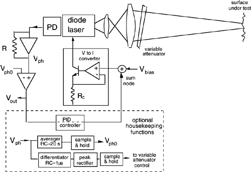
This is a small value as compared to perhaps I_dc=30-70 mA of normal rating current of our laser diode. We may take advantage of this circumstance by allowing a much larger current regulation range, e.g., I_reg=8 mA. Therefore, we may recover a large number I_reg/ΔI=50 of 2π-phase periods, or, equivalently a λ(I_reg/ΔI)=40μm drift, still keeping the linearity at the best half-fringe value.

The upper limit to I_reg is the incipient mode hopping, depending on the specific laser and ≈10 mA in best units with a TEC control of chip temperature (App.A1.3.1).

About the frequency response of the current-actuated half-fringe feedback loop, the theoretical limitations are: (i) the 2s/c delay (typ. a few ns), (ii) the laser response, involving the τ_p and τ_s time constants (ps to ns, see Sect.4.5.2.6), and (iii) the frequency response of the electronics, including front-end and laser drive-circuit response.

This response can be readily designed to exceed 10 MHz.

The output signal can be taken from the output of the transimpedance, proportional to the current error signal ΔI. Indeed, from Δ(2ks)=-2skΔλ/λ+2kΔs=-2ks α_IΔI+2kΔs, we can solve for Δs as Δs=sα_IΔI. This equation reveals that the instrument shall be calibrated once for all against the current coefficient α_I and in the actual use against the distance s.

Experimentally, the scale factor 1/sα_I = ΔI/Δs fairly well matches the 1/s dependence (see Fig.4-37) and is well reproducible (with a <1% error) from measurement to measurement.

In the practical implementation of the injection vibrometer, a few refinements are worth addition, as outlined in Fig.4-36.

Fig. 4-37 The scale factor of the output signal from the injection vibrometer. Line: theoretical 1/s dependence; points: experimental values.

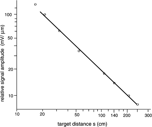
A PID controller (a network, well known in control technique, including a gain trimmer, a low-pass, and a high-pass filter) can be inserted to optimize the frequency response of the regulated loop. Also, an automatic reference circuit, made by a long time-constant averager and a sample-and-hold can be used to avoid readjusting the reference V_ph0 when optical power changes.

Last, to track the 1<C<4.6 condition against distance and target diffusivity coefficient, a control of the variable attenuator may be envisaged.

The performance of an instrument developed [30] with the half-fringe stabilization concept and operating in the injection regime described previously, are shown in the diagrams of Fig.4-38. Limit sensitivity is down to , and the maximum amplitude is about hundred μm (in total, six decades in amplitude dynamic range). A frequency response of up to hundreds of kHz is covered.

The linearity of the measurement is better than 1% as a deviation measured from true s(t). Also, the instrument operates on untreated target surfaces with diffusivity as low as 0.3 [30].

Fig. 4-38 Performance diagram of an injection vibrometer, stabilized to half fringe, operating on a diffusing target surface [30]. The laser source is a 25 mW near infrared (λ=780 nm) commercial laser diode. Left: at a representative s= 80 cm distance, amplitude of vibration is measured up to >100kHz with 100 nm (or better) resolution (bandwidth is B=1Hz) and up to 100 μm as limited by the dynamic range of the fringe tracking circuit. Right: at a representative 100 Hz signal frequency, resolution is 0.1 to 1 nm (B=1 to 100 Hz) from s=30 to 250 cm, still with up to 100 μm maximum amplitude.

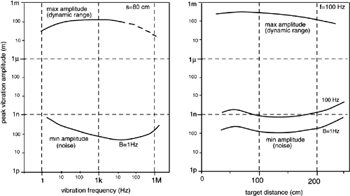
4.6.2.2 A plain injection vibrometer

In some circumstances, fringe stabilization at C>1 is unwieldy, either because the target diffusivity is very low or the laser diode has a long cavity and small spot size. Another reason is that we may want to trade performance for low cost and layout simplicity while retaining the basic advantages of the injection concept (self-alignment, self-filtering, etc).

Then, we can simply arrange for a minimum-count injection vibrometer made by an optical section including a diode laser, an objective lens, and an attenuator, and an electronic section made by the front-end preamplified connected to the laser monitor photodiode.

With this arrangement, we get the plain interferometric signal I_ph=I₀(1+cos 2ks), where s=s_m(t)+s_micr(t), s_m(t) is the useful vibration signal and s_micr(t) is the ambient-induced microphonics. As previously noted, we can separate these two addends if they lie in different frequency bands. Also, the cosine ambiguity is no problem if we look to a sinusoidal vibration s_m(t), especially if the s_m(t) swing has a multi-λ amplitude. The s_micr(t) disturbance then helps avoid the signal to be pinned at the 2ks=nπ worst condition.

An example of application of the approach is provided by a prototype instrument intended for MEMS testing [31], shown in Fig.4-39. The beam is focused on a MEMS Si-chip, typically 500μm by side, incorporating a comb-like spring structure and a mass, to diagnose the mechanical properties of the structure. The mass is aimed at by the focused laser spot (typ. 100 μm), but, even if some nonmoving parts are illuminated, by virtue of the injection process, they do not disturb the detection of the useful signal.

In the measurement setup (Fig.4-39), the MEMS is mounted inside a vacuum chamber to be able to test it at different ambient pressures. The window of the glass chamber does not need to have a good optical quality, because the wave front distortion is just a small additional attenuation, tolerated by the injection vibrometer. The out-of-plane vibration of the MEM mass is viewed at an angle Φ (≈20° in Fig.4-39), and the appropriate cos Φ correction on s(t) is applied to the measurement.

Fig. 4-39 Setup for measuring the mechanical properties of a Si-MEMS by means of an injection vibrometer. Light from the laser is focused on the vibrating mass of the MEMS chip through the glass wall of the vacuum chamber (from [31], by courtesy of IEEE LEOS).

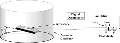
The signal out from the preamplifier is acquired by a digital oscilloscope, and the desired s(t) waveform (Fig.4-40) is computed from the I_ph=I₀[1+cos(2kA₀cosω₀t)], by means of a routine minimizing the rms errors of the desired quantities, amplitude A₀ and frequency ω₀.

Fig.4-40 The MEMS drive signal (square wave) and the interferometric signal output I_ph=I₀[1+cos(2kA₀cosω₀t)], as obtained from the vibrometer of Fig.4-39.

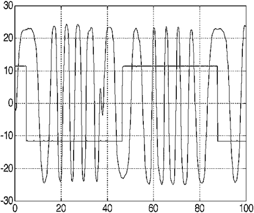
By sweeping the drive signal frequency, we can measure the frequency response of the MEMS in several conditions of interest and test the dependence on drive voltage and ambient pressure. Experimental results in Fig.4-41 show the effect of increasing drive voltage (and vibration amplitude). The response is linear for low V, but shows incipient hysteresis at V=8-9 Volt, indicating the risk of creep in the structure. Also, the effect of damping of the mechanical Q-factor because of insufficiently low ambient pressure is clearly evidenced.

Fig.4-41 The MEMS frequency response, as measured by the injection vibrometer (horizontal scale in kHz, vertical scale in relative units). Left: at increasing drive voltage up to incipient hysteresis; right: at different ambient pressures up to Q-factor damping (from [31], by courtesy of IEEE LEOS)

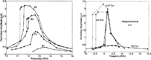
4.6.3 Long-Distance Vibrometry

Early experiments in long-distance vibrometry were aimed to remote, noncontact diagnostics of large structures, like towers, bridges, and other construction hardware of industrial, civil, or historical interest. Since the 1970s, several instruments have been developed internationally by several research centers [32].

To circumvent the ambiguity, around 2ks=0 or π, of the baseband cos2ks signal, the approach selected has been that of a heterodyne detection of the remote target echo. This is equivalent in performance, with other parameters being equal, to the homodyne with the half-fringe tracking approach discussed previously, and is much akin the two-frequency interferometer (Sect.4.2.2).

Of course, as a source adequate for long distance operation, we need a frequency-stabilized laser with a coherence length in excess of the distance 2s to be covered. For s≈300 m, this requires a laser linewidth Δν=c/2s=500 kHz or better. Also, the power should be adequate to allow for an increased attenuation, which calls for units with power typically in the range 20 to 50 mW (He-Ne) or ≈1 W (CO₂).

The basic configuration to start with is illustrated in Fig.4-42. The source is a single-mode frequency-stabilized laser (He-Ne or a CO₂ for larger distances). The beam is sent to a beamsplitter, and one output is directed to a telescope aimed to the target, while the other is used as the local oscillator for heterodyning. To get a frequency-shifted reference, an acoustooptical modulator (or Bragg cell) is used and provides an output shifted by Δω =10-50 MHz typically.

Fig.4-42 Scheme of a long distance vibrometer. The frequency-stabilized laser is frequency-shifted by a Bragg acoustooptic cell to generate a reference local oscillator. A beamsplitter (BS2) is used for beam recombination on the balanced detector. The mixer brings the signal to the base band.

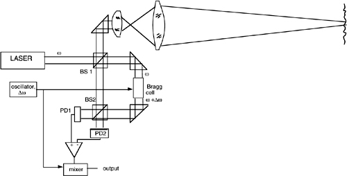
After propagation to the target and back, the optical signal is collected by the telescope and superposed to the local oscillator with the aid of a second beamsplitter BS2, ending on a balanced detector (see Ref.[5], Ch.8.2). Here, by beating of the fields, we obtain the photodetected signals as I_ph1=(I₀/2)[1+cos(Δωt+2ks)] and I_ph2=(I₀/2)[1-cos(Δωt+2ks)] and, after subtraction, we get S= I₀ cos(Δωt+2ks). By mixing it with the original frequency difference Δω or a fraction of it, the vibration-signal 2ks=A₀cosω₀t is brought to the baseband (or to an intermediate frequency) for further processing.

Several improvements can be introduced in the basic scheme of Fig.4-42. First, the beamsplitter BS1 halves the optical signal returning from the telescope and directs half of it back into the laser. We can eliminate this return by using a Glan-polarizing beamsplitter for BS1 and by adding a polarizer before entering BS1.

Second, superposed to the useful signal coming back from the target, we find a backscattering contribution, generated by the atmosphere along the propagation path. This contribution can even be larger than the useful echo when distance increases. To get rid of it, we may take advantage of the polarization properties of scattering, by which a propagating circularly polarized (CP) beam (say right-handed, RH) scatters back a left-handed (LH) contribution. In contrast, the target depolarizes the echo for any impinging state of polarization, and the useful returning signal contains as much RH as LH power. We may use a CP beam in transmission and cut off the back-scattered power by adding a polarizer and a quarter-wave plate at the telescope entrance. If the laser beam has a linear polarization and we align it to the polarizer, no loss in transmission will be experienced, while the back-scatter power will find the polarizer in the crossed state and be eliminated. The outgoing CP signal is then combined at the balanced detector, again using a Glan beamsplitter for BS2, with the reference beam either in a CP or in a linear, 45°-oriented state.

To protect the frequency-stabilizer laser source from even minute, unwanted reflections eventually originated in the optical devices internal to the instrument, we may consider adding an Optical Isolator (OI) at the laser beam output. The OI is well-known device, based on magnetooptical nonreciprocal rotation and is widely used for protecting lasers in fiber-optics communications. It has ideally a T=1 transmission in one direction, and T=0 in the reverse direction. Versions of OI without fiber pigtails (called free-space OIs) are readily available in the wavelength range λ=850-1600 nm of interest for fibers, while materials for the visible range are rather exotic and may not be easily available (at reasonable price).

Still another magnetooptical device may be useful, the Optical Circulator (OC). As an evolution of the OI, the circulator has four access ports for the beam. A beam entering in the i-th input exits from the (i+1)-th port with T=1 transmission, while it is T=0 for all other ports. Placed at the entrance of the telescope, the OC provides us with an input and output port spatially (or physically) separated without introducing any loss, which is different from normal beamsplitters. The OC also eases the layout of transmitted and received beams and cuts out unwanted reflections and scattering.

The typical sensitivity performances (or, NED) of a vibrometer built around the hetero-dyne concept are reported in Fig.4-43. As it can be seen, sensitivity is dominated at low frequency (<100 Hz) by an excess noise. This is due to turbulence effects, overwhelming the fundamental, flat-spectrum shot noise and electronics noise, which is finally reached at higher frequency (≈1kHz).

Fig.4-43 Typical NED of a long-distance vibrometer, as a function of frequency, for the detection of small remote vibrations on a diffusing target with He-Ne and CO₂ lasers. Operation is at s=100m distance, B=1Hz, in a clear atmosphere.

As outlined in App. A3, turbulence introduces a random fluctuation of the index of refraction and hence of the optical path length summed to the useful vibration signal. In addition, we find beam wandering around the aiming direction and distortion of the wave front in form of scintillation or bright spots. Both effects combine with the speckle regime of the remote-diffusing surface to add an error.

Thus, operation of the vibrometer on substantial distance (say, in excess of a few tens of meters) requires taking care of propagation condition to keep turbulence effects low.

We can try to mitigate or almost compensate for these effects of turbulence by electronic and optical, as well as measurement strategies.

Electronically, we may subtract the spectrum of the fluctuations, in a measurement with the vibrodyne off, from the useful spectrum with the vibrodyne on. This helps reduce the noise floor at low frequency, perhaps by a factor of 10, but not better because turbulence is not strictly stationary, statistically speaking, in separate measurement sessions. By optical means, we can attempt to compensate turbulence with adaptive optics, theoretically up to a perfect cancellation, but practical schemes are rather involved and have not yet demonstrated a valuable improvement, so far. Last, we can take advantage of the variability of turbulence from day to day and in daily hours. By waiting for a calm day and the best hours to carry out the measurement, turbulence effects are greatly reduced. This strategy is indeed acceptable when evaluating the structural integrity of buildings, which requires an outcome be determined within, say, a few days rather than instantly.

In performing the measurement, we should prefer operating on the shortest distance that is practicable. As a rule of thumb, if the article we are going to test has an out-of-ground height H, we will position our instrument at a distance d≈H to be able to test the bottom and top parts of it in a single session (Fig.4-44).

To generate a test vibration, a vibrodyne is used, which is fastened securely atop the structure. The vibrodyne is an electromechanical device consisting of an electrical motor (typ. ≈50 W in power) with an eccentric-mounted mass (typ. ≈1 kg) rotating at a frequency f_vib (typ f_vib≈0.1 to 10 Hz). Because of the mechanical torque generated by the vibrodyne, even a modest mass like 1 kg readily generates amplitude of displacements 10 to 100 nm in the tower top surface.

Of course, this amplitude is well within safety limits, and corresponds to the natural stress imparted by a moderate wind (say, with a speed 0.1 to 1 m/s).

The test session consists of measuring the vibration amplitude on a number of points selected along the structure and repeating the measurements for a set of frequencies covering the natural vibration frequencies of the structure. For the simplest article, a tower, we may take, for example, 10 sampling points in H/10 steps, and 10 frequencies, from a fraction (e.g., 1/4) of the lowest-mode frequency f₀ to 10 times as much, in equally log-spaced steps.

In this way, we are able to obtain the frequency response F(h,ω) to a mechanical excitation, a response which is resolved spatially. Now, the measured frequency response can be compared with what is expected from a solid structure, as calculated by standard methods well known in structural engineering. Also, we may introduce modifications in the calculation to simulate the effect of localized flaws and yields for ease of comparison.

Let us consider an illustrative example. A tower or chimney has bending modes at frequencies , where n=1,3,5… is the order of the mode, k is the elastic constant (N/m), M is the mass, and η is a dimensionless factor depending on height, diameter, wall thickness, etc.

Fig. 4-44 Arrangement for testing a tower by means of a laser vibrometer and a vibrodyne

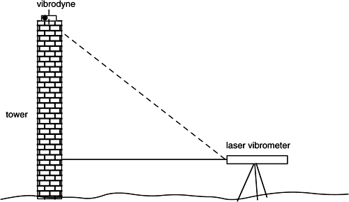
Fig. 4-45 Top: a tower or chimney has bending vibration modes with nodes (indicated by points) and antinodes (arrows) at integer fractions of the height H. The modes are revealed by the frequency response (bottom) taken at different heights h.

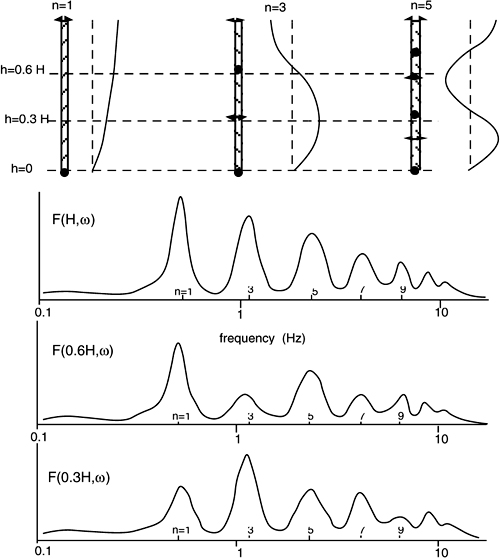
The lowest mode has a node of vibration at h=0 and an antinode (or maximum swing) of vibration at h=H, or, the standing wave of vibration has half-period in the height H. Higher order modes have n/2 periods in H (see Fig.4-45). Additional modes can be found in a structure lacking radial symmetry or having finer structural details, but here we ignore them for simplicity.

The frequency of the n=1 mode is found at f₁=0.02 to 1 Hz, typically (Fig.4-45), in most practical cases of interest (10 to 50 m towers). Higher modes have resonant frequencies that are odd-multiples of the fundamental one.

As a function of height, the amplitude of vibration changes with the mode order (Fig. 4-45), and we can therefore recognize them by looking at the relative obtained at different heights. The sharpness of the resonance decreases with the order of resonance and, more important, with the deviations from the structural integrity of the article. A solid structure has a well-defined resonance spectrum, whereas a near-to-collapse article usually exhibits a broad spectrum of frequency response F(h,ω), with a barely recognizable resonance pattern.

Fig. 4-46 Vibration measurement (top) and the result after background subtraction (bottom), revealing the state of conservation by means of the resonance spectrum

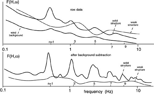
The raw interferometric signal of the vibrometer has a frequency spectrum with a strong background due to turbulence (Fig.4-46). After background subtraction through a separate measurement with the vibrodyne off, the resonance peaks of a solid structure are clearly highlighted. For a weak structure, the spectrum is rather flat without the expected resonances, and the measurement of the frequency response F(h,ω) at various heights adds further evidence.

At a closer look, in the background spectrum due to wind and turbulence we find, for a solid structure, modest peaks at resonances (Fig.4-46, top). This can be explained because the wind is a sort of white-noise excitation of the structure, and the mechanical response is enhanced at resonance. Thus, under favorable circumstances—a wind strong enough to impart a mechanical excitation to the structure, but not so strong to overwhelm the useful signal by turbulence—we can dispense with using the vibrodyne and need not climb the article to mount it.

Subtraction of the background cannot be performed as it was previously, in this case. However, from the set of measurements at different heights, and knowing the relative amplitudes of the expected resonances, we can process the data as to subtract the common background with a least-mean-square error routine, for example.

In conclusion, despite the limitation of turbulence, long-distance vibrometry offers a powerful diagnostic tool for noncontact testing of buildings. This is exemplified by examination of masterpieces like the historical Pisa tower [33] and similar articles, as well as in the diagnostic of structural integrity of industrial articles, notably cooling towers and chimneys of cement factories, electrical generating plants, and the like.

About the choice of the wavelength best suited for long-distance operation of the vibrometer, let us consider the factors involved, by comparing He-Ne (λ=0.63 μm) and CO₂ (λ=10.6 μm) lasers. The turbulence-induced Δn fluctuation and the phase noise (App.A3.2) is proportional to σ_χ∝λ^-7/12, thus noise decreases of a factor (λ_He-Ne/λ_CO2)^7/12=0.24 going to the infrared.

The NED is proportional to wavelength and to (S/N)^-1 ratio, on its turn proportional to λ: so we get an increase of it by in the IR.

Optical device transmission and detector quantum efficiency η are worse in IR as compared to visible, and we may take a factor ≈3 of increase in the IR.

Last, power available from a small CO₂ laser is readily ≈1W, instead of 50 mW of a He-Ne laser, and this gives a factor of NED decrease in IR.

Collecting the contribution, the NED we should expect in IR is 0.24^·0.4^·16.8^·3^·0.22=1.06 times that of the He-Ne, or, substantially the same. However, the effects of turbulence are smaller in the IR, as indicated by Fig.4-43 where the corner frequency of noise for the CO₂ wavelength is smaller.

4.7 Other Applications Of Injection Interferometry

Recently, a few additional applications of injection interferometry have been reported [34], which are particularly attractive, though they are still at the development stage and not yet incorporated in commercial products, like those found for the other topics discussed in this chapter.

4.7.1 Absolute Distance Measurements

Laser interferometry is intrinsically a phase-difference tool, and is definitely the best for high-resolution measurement of displacements with sub-λ increments, but it requires a moving target sliding along the displacement to develop the counts. On the other hand, telemeters based on beam modulation (Chapter 3) can operate on still targets and are truly absolute distance meters.

However, because interferometry works at the quantum limit of sensitivity and the injection configuration is especially very attractive for its simplicity, we may try to devise a scheme circumventing the basic limitation of incremental measurement.

The starting point is to sweep the wavelength of the source, a feature readily available in diode lasers through modulation of the drive current (App.A1.3). Sweeping the wavelength changes the number of wavelengths N=2s/λ contained in the go-and-return path to the target. Each time one more wavelength fits in 2s, the interferometric signal undergoes a 2π phase shift (and a switch in the C>1 injection regime). By detecting it, we may be able to trace back the absolute distance s.

As a wavelength modulation, let us now consider a linear sweep on a swing Δλ.

This modulation is obtained by superposing a linear sweep on the drive current, with an amplitude ΔI=Δλ/α_I (App.A1.3) superposed to the quiescent dc current I_dc. The interferometric signal I_ph/I₀=1+cos 2ks at the start and at the end of the sweep period is, respectively:

I_ph/I₀= 1+ cos 4π s /λ₀, and

I_ph/I₀ = 1+ cos 4πs/(λ₀+Δλ) ≈ 1 + cos 4πs (1-Δλ/λ₀)/λ₀

Thus, the phase variation ΔΦ produced by the sweep is:

ΔΦ= 4πs(1-Δλ/λ₀)/λ₀-4π s /λ₀= -4π s Δλ/λ₀²

By dividing ΔΦ by 2π, we get the number of interferometric waveform periods found in the photodetected current as N= 2Δλ/λ₀²s. For C>1, N is the number of switchings to be counted. From N, the distance is obtained as:

(4.55)

Each count (N=1 in Eq.4.55) corresponds to a distance Δs=λ₀²/2Δλ, and this represents the resolution of the measurement performed in the injection regime (Sect.4.5.2), with C>1. In a normal Fabry-Perot laser, the practical limit to the wavelength swing we may impose with a reasonable excursion of the drive current is Δλ≈4nm (Fig.A1-13), and thus the theoretically attainable resolution at λ=1000 nm can be estimated as Δs=(1000)²/2.4 =125 μm, a very attractive value indeed.

Unfortunately, Fabry-Perot laser diodes are affected by mode hopping (Fig.A1-13) at large Δλ swings. Though not a really fundamental limitation, mode hopping is detrimental to signal processing and, to avoid it, reported experiments [35] limit the useable wavelength swing to about Δλ≈0.2nm, so that the resolution presently attained is about Δs≈ (1000)²/(2.0.2)≈2.5 mm, up to a distance s of a few meters.

An experimental arrangement is shown in Fig.4-47. A triangular modulation is applied to the laser drive current. This produces a wavelength modulation and, in addition, also a power amplitude modulation of the same waveform. We can subtract the power-dependent term, however, using a fraction of the modulating signal, eventually slightly distorted so as to correct for the P=P(I) non-linearity of the laser diode characteristics.

After the subtraction, we obtain the interferometric signal S(t) (Fig.4-47) and one full period for each ΔΦ=2π change. In the injection regime with C not too small, the leading edge is faster than the trailing edge. Thus, by time-differentiation, we will get pulses with the positive part larger than the negative one, easily discriminated. To count the positive pulses during the Δλ sweep time, we may simply differentiate the modulating waveform (Fig.4-47) and use it as a gate signal for the counter.

The number of counts N is used in Eq.4.55 to determine the distance s, with a scale factor given by λ₀²/2Δλ.

Two sources of error shall be considered. First, because of the discrete counting process, we incur into a ±1 count as round off error at the beginning and end of the sweep.

As an average, the systematic error is +1-1=0. Recalling that the variance of a uniform distribution is 1/12, we have a random rms error σ_dis=√(1+|-1|)/√12=1/√6 counts. This error is reduced by a factor 1/√N_T if we repeat the measurement N_T times, provided the initial phase is randomly distributed between 0 and 2π [ambient vibration superposed on s usually suffices for that].

Fig. 4-47 Absolute distance meter based on injection interferometry. The laser wavelength is swept with a triangular waveform, using a current modulation superposed to the bias I_bias. The photodiode signal, after subtraction of the power-dependent term duplicating the modulation, exhibits spikes corresponding to ΔΦ=2π variations. Counting them, the distance is found as s=N λ²/2Δλ. To improve the measurement accuracy, we may add the section with the beamsplitter and the Fabry-Perot to count N_ref=2L_FPΔλ/λ² with a separate circuit (not shown in figure) and get Δλ= N_refλ²/2L_FP, and accordingly s= (N/ N_ref) L_FP.

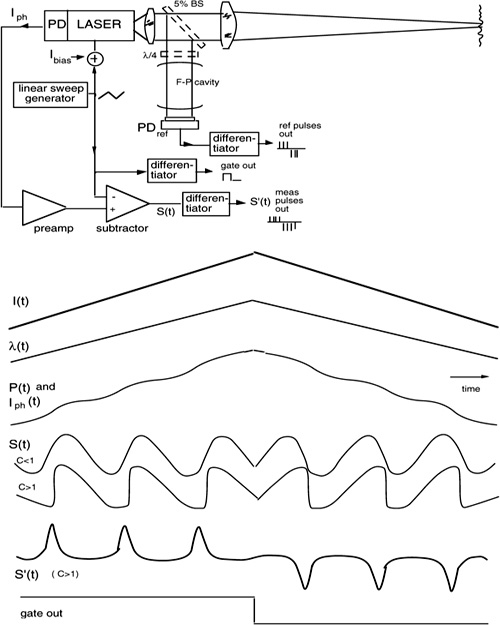
Second, the accuracy of the scale factor depends on how precisely we know λ₀ and Δλ. Usually, wavelength is known to better than one part in 10³, whereas Δλ may scatter by as much as a few percent around the nominal value α_IΔI.

An elegant method to circumvent the accuracy problem is illustrated in Fig.4-47. We pick out a fraction (say, 5%) of the power projected on the target by a beamsplitter and send it to an interferometer. The interferometer may be a Mach-Zehnder as first reported in [36], or a Fabry-Perot for a simpler implementation as shown in Fig.4-47. Feeding the interferometer under the wavelength sweep, we get a periodic sequence of signal peaks at the output (see Fig.A2-2), with a period c/2L_FP in frequency and λ₀²/2L_FP in wavelength. Now, we need only to duplicate the circuit of the main section to read these peaks. Counting them, we get a total number N_ref=2L_FPΔλ/λ² in a sweep, where L_F-P is the cavity length of the Fabry-Perot (which is known to a very good accuracy).

Using the scale factor 2Δλ/λ²=N_ref/L_FP in Eq.4-55, we now can obtain the desired distance as s= L_FP(N/N_ref), that is, we are completely released from the λ and Δλ. Note that the interferometer needs a length L_FP comparable to the distance s if the count discrete error of it is to remain low.

4.7.2 Angle Measurements

Alignment of mirrors along the line of sight defined by a laser-beam wave vector is one of the early applications reported [37] for injection interferometry.

Fig. 4-48 Alignment of a remote mirror to the propagation wave vector k of the laser: ambient vibrations provide an interferometric signal, whose maximum is found when the error angle α is at a minimum (typ. <3 arcsec).

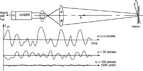
Fig.4-48 shows the straight arrangement for such an autocollimator measurement. The laser beam is expanded by a telescope and sent to the mirror target. On a substantial distance (say, >30 cm) the normal ambient-induced vibrations readily provide an interferometric signal, for which the amplitude is maximum when the alignment is best.

More specifically, the maximum is attained when the angle error α is fairly less than the diffraction limit of the transmitted beam, with a typical resolution <3 arcsec as indicated in Fig.4-48.

Like working with a normal optical autocollimator, the alignment of several reflecting surfaces is achieved by separately aligning each surface to the k vector, used as an angular yardstick.

The injection-interferometer autocollimator has been found useful in alignment with IR lasers (originally, with a 3.39μm He-Ne laser). However, it does not provide a true angle measurement, but just a sensitive null detection.

By adding a line-of-sight modulation to the basic scheme, we can work out a true angle measurement. The beam can be steered by an actuator, e.g., an x-y translation of the laser chip or of the first lens of the telescope, or by means of a prism inserted in the transmitted beam. To substantiate the design, let us assume a deflection Δx=Δx₀cosω₀t of the first lens. Then, the angle of k is modulated with a deflection α=Δα₀cosω₀t, where Δα₀=Δx₀/F and F is the focal length of the first lens. As illustrated in Fig.4-49, with no modulation the response versus α is parabolic, whereas adding the modulation and using phase detection, the response is linear up to the amplitude Δα₀ of the angle swing.

Typical performance of the angle meter implemented with a laser diode in the injection-interferometry configuration [38] is a noise-limited resolution of ≈0.2 arcsec on a ≈5 arcmin dynamic range.

Fig. 4-49 Angle measurement by injection interferometry: the aiming direction is modulated so that the parabolic amplitude response is transformed into a linear dependence on the angle α₀ to be measured.

4.7.3 Detection of Weak Echoes

Besides the phase difference φ_m-φ_r, the generic interferometric signal (Eq.4.2) contains information on the amplitude of the field E_m returning to the measuring port. Actually, any interferometer can be regarded as a coherent detection scheme (see [5], Ch.8) in which E_m is the signal and E_rE_m is the local oscillator. By beating of the fields E_r and E_m at the photodetector, an internal gain is generated, and the quantum limit of detection is attained. Thus, as an amplitude detector, the interferometer has the advantage of a very good sensitivity to small signal and echo returned after a strong attenuation.

The coherent detection scheme is classified as homodyne or heterodyne according to whether f_m=f_r or f_m≠f_r and as an injection scheme if the returning signal is fed into the source. Classical homodyne or heterodyne detection is used in fiber optics communication, whereas injection detection is attractive in instrumentation because of several features (Sect.4.5.2.5).

Using Eq.4.52, we can write the photocurrent signal i_ph=σΔP of the self-mixing configuration in the weak-injection regime as:

(4.56)

Here, I₀=σP₀ is the dc photocurrent, κ=cτ_p/n_lL is a constant of the order of unity, and a is the total (field) loss in the path to the target at distance s and back, explicitly a=√A in terms of the total power attenuation A.

Eq.4.56 tells us that, at weak injection levels (a1), the signal has an amplitude proportional to the square root of power attenuation, a=√A, as expected from a coherent detection process. When κa≈1 or C>1 (moderate feedback), the amplitude does not increase any more and we get a saturation of the signal versus attenuation (Fig.4-50).

Fig. 4-50 The theoretical dependence of signal amplitude from external attenuation (or return loss) in an injection interferometer, for some values of distance.

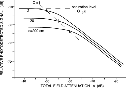
To be able to measure the amplitude I₀κa without being disturbed by the phase term cos2ks, we need either the distance to be a constant or to be varying in a known way. If we are operating on a substantial distance (say s >50 cm), ambient-related microphonics usually contributes with a random jitter s_j(t)λ added to the mean s, and therefore cos2ks is a random waveform with zero mean value and a rms value 1/√2. Then, we will measure the rms i_ph value of the signal and get the attenuation as a=√2i_ph(rms)/I₀κ.

If distance is short or we want to move the signal off the dc, we may add in the optical path a phase modulation Φ=Φ₀ cosω_mt, with a deviation Φ₀>2π large enough to have a phase term cos(2ks+Φ) swinging from –1 to +1. In this way, the signal is modulated on a carrier frequency ω_m, at which the measurement of amplitude will be performed.

Typical examples of echo attenuation measurement [39-41] are shown in Fig.4-51. The first setup [40,41] is for the measurement of the return loss from a fiber device (DUT, device under test). The optical path length is modulated with the aid of a piezoceramic (PZT) phase modulator driven at frequency ω_m, and the output signal at frequency ω_m is proportional to the square root of the ratio P_back/P₀=A_RL. In this scheme, we may also add a second photodetector PD2 to measure the ratio P_tr/P₀, of the DUT, that is, its insertion loss.

Fig. 4-51 Typical arrangements for the measurement of weak echoes by self-mixing interferometry. Top: for measuring the return loss of an all-fiber device (DUT), we can use an in-line PZT phase modulator. Bottom: for testing the isolation of an optical isolator mounted in the laser package, a remote vibrating mirror mounted on a loudspeaker supplies the path length modulation.

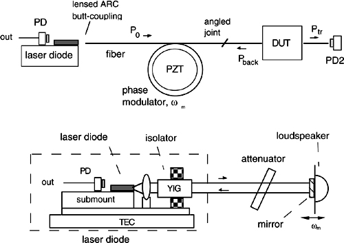
In the second example, aimed to test the isolation factor of an optical isolator mounted in front of the laser chip [39], we shall use a path-length modulation external to the device. This can be a mirror aligned to the transmitted beam and mounted on a loudspeaker, driven at the desired frequency ω_m. In this case, the signal is proportional to the square root of the isolation factor P_back/P₀.

To make the point clear, 10 dB (or a decade) of attenuation corresponds to a half a decade of variation in the current or voltage signal, that is, to a 10 dB change in it.

Typical performances of the echo detector based on the injection interferometer are illustrated in Fig.4-52. Several single-mode laser diodes operating at different wavelengths have been experimented, with either plain Fabry-Perot or DFB (grating reflector) structure. For all of them, the range of measurable attenuation spans from –25 dB to –80 dB. By adding an attenuator in the optical path (Fig.4-51, bottom), we can extend the upper limit to about 0 dB.

Fig. 4-52 Typical attenuation or optical isolation that can be measured by a diode laser operating in the injection interferometer regime of echo detection. At about -80 dB the limitation is S/N ratio, whereas at ≈-30 dB is saturation.

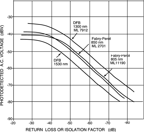
Other interesting applications of the echo detection by injection-interferometer schemes have been reported in the fields of optical testing [42], compact-disk readout [43], and scroll sensors [44].

In CDs, optical pits correspond to the bits of recorded information. In conventional design, to read the bits we need a laser and photodiode combination, a beamsplitter to divide the input and output beam paths, and a conjugating lens to focus on the spot.

Using an injection detector, we can dispense for the beamsplitter and the lens (Fig. 4-53) by placing the laser diode close to the disk (typically at 10-20 μm off the surface). The rear photodiode will supply the readout signal in form of spikes corresponding to the bits superposed to the dc quiescent current [43].

Fig. 4-53 Readout of optical bits in a CD by injection interferometry. The laser and photodiode combination provide a readout signal. Unwritten portions of the CD surface reflect light and give a large signal, whereas pits diffuse light and give a small injection signal detected by the rear photodiode.

Another recently reported example of an application of the readout of echoes by injection interferometry is the scroll sensor [44]. The scroll sensor is used in mobile telephone sets and is one of the two axes of the computer mouse. It supplies a signal indicating the up/down direction of a finger or another common surface presented at the viewing window of the sensor, and operates with no physical contact or a particularly clean window.

As shown in Fig.4-54, we can design a scroll sensor by means of two low-cost single mode lasers in a package with folding mirrors. The mirrors direct the beams on the output window. The incidence angles of the two beams are ≈45° and the sign opposite, so that the phase term 2k·s driving the self-mixing modulations (AM and FM) has an opposite sign in the two laser cavities.

As usual, we get the AM signal directly from the photocurrent of the monitor photodiode mounted in front of the rear mirror of each laser. Using a difference amplifier to subtract the two signals and time-differentiating the result, we obtain a signal with a polarity which indicates the up/down direction of the scroll, and with an amplitude which is proportional to the speed 2k· s’. The external surface we sense does not need to be treated or be in contact with the window.

As wavelength of operation, a visible (typically 620 to 680 nm) wavelength is preferred because of safety issues (App.A1.5), and because the laser power requirement is modest (≈0.2 mW or less).

Fig. 4-54 In a self-mixing scroll sensor, two low-cost lasers shine on the sensing window, with beams impinging there at an angle (typically 45°) from opposite sides. The self-mixing signal 2k·s returned to each laser cavity is then opposite in sign. After detection on the monitor photodiode, subtraction of currents yields the direction of surface movement.

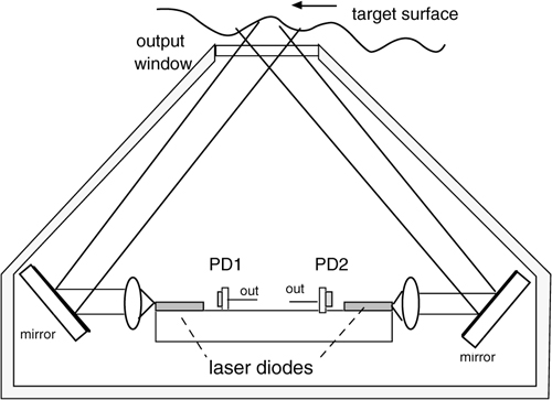
4.8 White Light Interferometry

In all applications of laser interferometry described so far, we have called for sources with a long coherence length. Indeed, operation is intended in the coherent regime of superposition of reference and measurement fields so that we can resolve sub-λ path-length differences. Indeed, if we have to accommodate an arm-imbalance 2(s_m-s_r) and yet get a nonvanishing interferometric signal, we need a coherence length l_c>2(s_m-s_r).

In white-light interferometry, this concept is completely overturned.

We use a low-coherence length source, like an LED, a Superluminescent LED (SLED), or a filtered incandescent lamp with a line width so large (Δλ≈20-100 nm around λ≈1μm) that the coherence length is limited to a very small value like l_c=λ²/ Δλ≈10-50μm.

Now, we extend the strategy of operation by looking at both the incoherent and coherent regimes of superposition. For 2(s_m-s_r)>l_c, the superposition is incoherent and the photodetector yields a dc current which is just the sum of the intensities provided by the reference and measurement beams.

On the other hand, when the arms are nearly balanced, 2(s_m-s_r)<l_c, the photodetector yields the interferometric beat signal added to the previous dc level.

Thus, by waiting for a spike to appear in the photodetector output signal, we are able to distinguish the balance condition s_m=s_r with a l_c≈10-50μm resolution.

Recalling Eq.4.12, we may write the photodetected signal from a Fabry-Perot interferometer in white light (Fig.4-55) as:

(4.57)

Recalling the result of Sect.4.4.2 and 4.4.3 and assuming a Lorentzian line, the visibility V can be expressed as: as:

(4.58)

To illustrate the practical implementation of the concept, let us refer to Fig.4-55.

Fig. 4-55 In a white-light interferometer, the interference signal only appears when arms are very close to balance (s_m=s_r±l_c) because the coherence length l_c is very short (≈20 to 50μm). The measurement condition is searched by scanning the reference arm length s_r, with the aid of a motorized translation stage and is revealed by a spikelike signal in photocurrent.

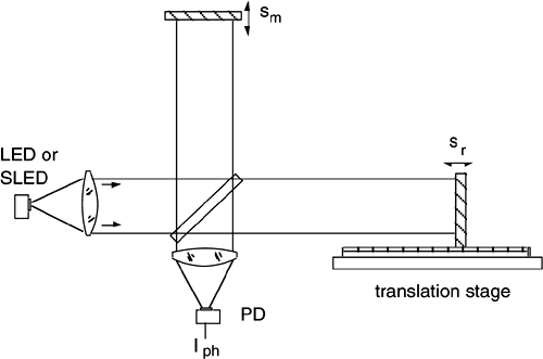
We may use either an LED or a SLED as the source of the interferometer. The basic SLED is a diode with a laser structure, but with the output mirror missing (the output facet is antireflection coated). Thus, laser oscillation is prevented and emission from the device is in form of spontaneous emission generated in the bulk and amplified down the path to reach the output facet, hence the name of superluminescent light.

The SLED has an emitted power (a few mW) and spectral width (typically Δλ≈20 to 50 nm) comparable to a normal LED, but emission is from a small spot size, nearly single-mode area, like that of a laser. Thus the SLED brilliance is high, which is a very useful feature. In view of Eq.4.58, the SLED is better because it has μ_sp≈1, whereas it may be μ_sp≈10^-3 for an LED. For the same reason, though in principle useable, an incandescent lamp source would provide a very low μ_sp≈1/N and useful signal, because of the large number of modes emitted (N≈AΩ/λ², see [5], App.A2).

The other factor in Eq.4.58 is usually μ_pol≈0.5 because either the source is unpolarized or polarization is not preserved in rediffusion from a rough target.

Considering a Fabry-Perot interferometer (Fig.4-55), one mirror is secured to the target being measured, and the other mirror is mounted on a precision translation stage. In this way, the reference arm can be scanned to search for the s_r=s_m condition while keeping the interferometer aligned. Of course, we can replace the mirrors with corner cubes to relax the angular alignment criticality and have much larger signal amplitude.

Now, as we pass through the s_r=s_m condition, oscillations corresponding to fringes show up in the photocurrent signal I_ph, as illustrated in Fig.4.56, in accordance with Eq.4.57. If the translation stage is moved with a constant speed, the waveform of I_ph versus time is a replica of the dependence versus s_r.

Fig. 4-56 The photodiode signal at the output of a white-light interferometer is an oscillation with a pulse envelope, peaking in correspondence to the balance condition s_r=s_m. The envelope width is about equal to the coherence length 1_c and determines the resolution of the measurement.

To accurately localize the spike position, we may implement the following electronic processing. The photocurrent signal I_ph is first rectified, thus obtaining its envelope. By time differentiation of the envelope, we get a zero crossing in correspondence of its peak. Finally, a zero crossing comparator provides the logic signal to sample the s_m value, and is then read by an encoder mounted on the translation stage. About the measurement accuracy, several systematic, as well as random sources, are to be considered. By analyzing them, it is found that the accuracy σ_m is a fraction of the response Full-Width at Half Maximum (FWHM), equal to 2 ln 2 l_c =1.4 1_c for a Lorentzian line. In practice, we can achieve an accuracy of 10 to 50μm, not as good as in a conventional interferometer, yet a respectable value that can be adequate in a number of applications.

As a comment, the main drawback of the white-light technique is that we need a moveable stage inside the instrument, covering a distance D equal to the range 0-D to be measured. The practical range of measurement is accordingly limited to, say a few tens of cm, at least in the basic configuration, and this makes the technique unsuitable for long-distance, general-purpose measurements.

Of course, we can add a fixed delay in the reference arm to extend the range. For example, a coil of single-mode fiber with objective lenses to focus the input beam and to colli-mate the output beam readily provides a compact device, which increases the path length by nL and the distance range to nL-nL+D.

This feature coupled to the inherent single-mode propagation in fibers, makes white-light interferometry very attractive [45] for optical fiber sensors (Chapter 9). Also, when the distance range to be covered is rather small (say <1 cm), the technique is easily implemented and can be extended to the image format, as described in next section.

4.8.1 Application to Profilometry

When incorporated in a microscope, the white-light interferometer provides a measurement of the surface height of the specimen, with a spatial definition determined by the size of the illuminating spot. By moving the spot across the specimen in a x-y raster arrangement, we can obtain a map of surface height or a profilometry of the surface [46-48].

Specifically, the surface under test can be either a polished or a rough surface. The working principle is illustrated in Fig.4-57. A light source (normally an incandescent lamp) is filtered in wavelength by a colored filter to choose the desired λ₀ and Δλ, and spatially by a pinhole to work with a nearly single-mode spatial distribution.

With a collimating lens, the beam is sent along the axis of the microscope with the aid of a beamsplitter (BS1). After passing through the objective lens focused on the specimen surface, the illuminating beam encounters a pair of optical flats acting as an interferometer (called a Mirau interferometer).

The first flat F has antireflection coatings on both surfaces and a small central obstruction, which is black (absorbing) on the upper side and metallized (reflecting) on the bottom side. The second flat is partially reflecting and acts as a beamsplitter (BS2) on one of its surfaces.

At BS2, a part of the beam is directed to the specimen and constitutes the measurement beam, whereas the other part is reflected toward F to be used as the reference beam. The portion of the reference beam falling on the central metallization of F is reflected back to BS2 where it recombines with the measurement beam returning from the specimen. The two superposed beams are collected by the objective lens in front of the photodetector PD.

The interferometer arms are balanced when the distances of the beamsplitter BS2 to the specimen and to the flat F are equal, or differ by less than l_c. This condition is checked by the signal I_ph of the photodetector (Fig.4-57).

To obtain the condition of balance, the flat F is moved by a micrometer motorized stage. With a phase detector, we are able to lock the stage position at the I_ph maximum, with an accuracy of a few hundredths of l_c. The corresponding resolution in surface height is well below the micrometer.

About the stage drive, we do not actually need a precise z-axis movement, but rather a precise measurement of it, as can be supplied by a sensor secured on it. The sensor may be one of the several, well-known linear-motion transducers (e.g., a differential transformer, a linear potentiometer, or even a low-cost interferometer), capable of sub-μm accuracy or better [49].

Fig. 4-57 Basic setup of a profilometer based on white-light interferometry. A first beamsplitter BS1 combines the illuminating and returned beams. The flat F and the beamsplitter BS2 act as a Mirau interferometer (F has a small central portion mirrored). The path balance is obtained when the distances of BS2 to F and to specimen are equal. This condition is searched by moving the z-axis drive until the I_ph has the spike shown in Fig.4-56.

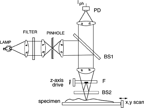
As the profile variations from point to point are usually small, and the moving part is of little weight, the time response of the system is adequately short, and acquisition of a single point may require t_r≈1-10ms.

The spot size is determined by the numerical aperture NA of the objective lens as s=λ/πNA (see [5], App.A2). This is the sampling dimension (or pixel minimum size) of the x-y profile measurement. As a typical value, for λ=0.5μm and NA=0.01-0.05, we get s=1-15μm.

To obtain a full-image profile measurement, a simple way is to move the specimen by a micromotorized stage in an x-y raster fashion. Again, precision encoders will provide the xy position readout to which the z-axis measurement is assigned. The total scan time of a 100×100 pixel image may be 10⁴×(1-10ms)=10-100 s, a fairly long but acceptable time.

Even better, we can use a CCD array as the photodetector to cover the full specimen image, and simply scan the z-axis. When an individual point in the specimen reaches the balance condition, the corresponding pixel will exhibit a current spike, and the z-measurement is assigned to the pixel coordinates.

A recent refinement to white-light profilometry has been that of improving the vertical resolution down to nanometers [50]. This is achieved by adaptation of the phase-shifting technique discussed in Sect.4.2.2.1 to the white-light interferometer scheme.

Fig. 4-58 A typical profilometer based on white-light interferometry (top) and two examples of images taken with submicrometer height resolution (courtesy of Zygo, Inc.).

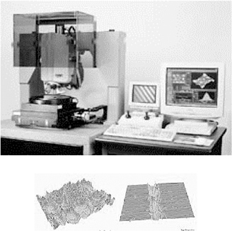
For points in the x-y plane close to the point under test, and deviating vertically by less than Δz<l_c, a fringe system is generated in the detector plane. Using a CCD, we can sample this fringe pattern and process the data in a computer. By successive acquisitions on overlapping spatial portions, the measurement is extended to the entire specimen.

A commercial profilometer is shown in Fig.4-58, along with typical examples illustrating the results of x-y profile measurements.

Another recent development in the field of white-light interferometry is Optical Coherence Tomography (OCT). In this technique, we produce the images of thin slices of the object under study, a biological tissue, or another semitransparent object [50], just by looking at it through a white-light interferometer. The reference length s_r (Fig.4-55) determines the depth, and the coherence length l_c determines the thickness of the slice.

References

[1] I. Newton, “Lectiones Opticae”, 1678 manuscript published in Cambridge, 1727; C. Huygens “Traité de la Lumiere”, Cambridge 1690; A. Schuster and J.W. Nicholson “Theory of Optics”, E. Arnold: London, 1904.

[2] A.F. Rude’ and M.J. Ward, “Laser Transducer System for High Accuracy Machine Positioning”, Hewlett Packard Journal (Feb.1976), pp.2-6.

[3] R.C. Quenelle and L.J. Wuertz, “A New Microcomputer Controlled Laser Dimensional Measurement and Analysis”, Hewlett Packard Journal (Apr.1983), pp.3-13.

[4] P.G. Halverson and R.E. Spero “Signal processing and Testing of Displacement Metrology Gauges with pm-Scale Cyclyc Nonlinearity”, J. of Optics A, vol.4 (2002), pp.S304-10.

[5] S. Donati, “Photodetectors”, Prentice Hall: Upper Saddle River, 2000.

[6] G. Molesini et al., “Multiphase Homodyne Interferometry”, Proc. Elettroottica’94, edited by S. Donati, pp.53-57, AEI: Milan, Italy, 1994.

[7] V. Annovazzi Lodi, S. Donati, and S. Merlo,“Thermodynamic Phase Noise in Fiber Interferometers ”, Journal Optical and Quantum Electronics, vol.28 (1996), pp.43-49.

[8] V. Annovazzi Lodi and S. Donati, “Injection Modulation in Coupled Laser Oscillators”, IEEE J. Quant. Electr., vol.QE-16 (1980), pp.859-865

[9] F. Aronowitz, “The Laser Gyro”, in Laser Applications, edited by M. Ross, Academic Press: New York, 1971, pp.134-199.

[10] S. Donati, “Laser Interferometry by Induced Modulation of the Cavity Field”, J. Appl. Physics, vol.49 (1978), pp.495-497.

[11] T. Bosch, N. Servagent, and S. Donati, “Optical Feedback Interferometry for Sensing Applications”, J. of Optical Engineering, vol.40 (2001), pp.20-27.

[12] A. Siegman, “Lasers”, University Science Books: Mill Valley, CA, 1986, pp.947-953.

[13] Y. Suematsu and A.R. Adams, “Handbook of Semiconductor Lasers and Photonic Integrated Circuits”, Chapman & Hall: London, 1994.

[14] R. Lang and K. Kobayashi, “External Optical Feedback Effects on Semiconductor Injection Laser Properties”, IEEE J. Quant. Electr., vol.QE-16 (1980), pp.347-355.

[15] S. Donati, G. Giuliani, and S. Merlo, “Laser Diode Feedback Interferometer for the Measurements of Displacements without Ambiguity”, IEEE J. Quant. Electr., vol.QE-31 (1995), pp.113 -119; also Italian Patent filed 18/10/94 n° PV-94 A00012.

[16] S. Donati and V. Speziali, “Laser Interferometry for Sensing of Respiratory Sounds”, Proc. CLEA Conf. on Laser and Electrooptics Appl., Washington, June 1977, Digest in IEEE J. Quant. Electr., vol.QE-13 (1977), pp.798-87D; also “Interferometric Sensing of Respiratory Sounds”, Laser & Elektro-Optik, Munchen, vol.12, 1980, pp.34-35.

[17] S. Donati, “A Novel Laser Interferometer for Distance Measurements”, Proc. Conf. on Precision Electromagnetic Measurements, Ottawa (1978), pp.75-77.

[18] N. Servagent, T. Bosch, and M. Lescure, “A Laser Displacement Sensor using the Self-Mixing for Modal Analysis and Defect Detection”, IEEE Trans. Instrument. Measur., vol.46 (1997), pp.847-850.

[19] S. Donati, L. Falzoni, and S. Merlo, “A PC-Interfaced, Compact Laser-Diode Feedback Interferometer for Displacement Measurements”, IEEE Trans. Instrument. Measur., vol.45 (1996), pp.942-947.

[20] K. Petermann, “Laser Diode Modulation and Noise”, Kluwer Academic: Dordrecht (Holland), 1988.

[21] G. Giuliani, P. Cinguino, and V. Seano, “ Multifunctional Characteristics of a 1.5μm Two-Sections Amplifier-Modulator-Detector”, IEEE Phot. Techn. Lett., vol.PTL-8 (1996), pp.367-369.

[22] S. Merlo and S. Donati, “Reconstruction of Displacement Waveform with a Single-Channel Laser-Diode Feedback Interferometer”, IEEE J. Quant. Electr., vol.QE-131 (1995), pp.113-119.

[23] P.J. de Groot, G. Gallatin, and S.H. Macomber, “Ranging and Velocimetry Signal in a Backscattering Modulated Laser Diode”, Applied Optics vol.27 (1988) pp.4475-4480; also Optics Lett., vol.14 (1989) pp.165-167.

[24] S. Shinohara et al., “Compact and Versatile Self-Mixing Type Semiconductor Laser Doppler Velocimeter with Direction Discrimination Circuit”, IEEE Trans. Instr. Measur. vol.38 (1989), pp.574-577; also IEEE Trans. Instr. and Measur., vol.41 (1992), pp.40-44.

[25] T. Bosch and M. Lescure (editors), “Selected Papers on Laser Distance Measurement”, SPIE Milestone Series, vol. MS115: Bellingham, WA, 1995.

[26] N. Servagent, F. Gouaux, and T. Bosch,“Measurement of Displacement using the Self-Mixing Interference in a Laser Diode ”, Journal of Optics, vol.29 (1998), pp.168-173.

[27] W.M. Wang, K.T.W. Grattan, A.W. Palmer, and W.J. Boyle, “Self-Mixing Interference inside a Single-Mode Laser Diode for Optical Sensing Applications”, IEEE J. Lightwave Techn. vol.LT-12 (1994), pp.1577-1587.

[28] R.S. Vodhanel, M. Krain, and R.E. Wagner, “Long-Term Wavelength Drift of0.01nm/y for 15 Free-Running DFB Lasers”, Proc. OFC-94 Optical Fiber Confer., San Jose, 20-25 Feb.1994, paper WG5, pp.103-104.

[29] R.O. Claus and C.H. Palmer, “Direct Measurement of Ultrasonic Stoneley Waves”, Appl. Phys. Lett., vol.31 (1977), pp.547-548.

[30] G. Giuliani, S. Bozzi-Pietra, and S. Donati, “Self-mixing Laser diode Vibrometer”, Meas. Sci. Technol., vol.14 (2003), pp.24-32.

[31] S. Donati, V. Annovazzi Lodi, S. Merlo, and M. Norgia, “Measurements of MEMS Mechanical parameters by Injection Interferometry”, Proc. IEEE-LEOS Conference on Optical MEMS, Kawai, HI, 21-24 Aug.2000, pp.89-90, see also IEEE J. Microelectromechanical Syst., vol.12 (2003), pp.540-549.

[32] M. Corti, F. Parmigiani, and S. Botcherby, “Description of a Coherent Light Technique to Detect Vibration of an Arch Dam”, J. Sound and Vibration, vol.84 (1981) pp.35-45.

[33] G. Macchi and A.Pavese, “Diagnosis of Masonry Towers Using Interferometric Transducers and System Identification”, in Proc. ODIMAP III, Pavia 20-22 Sept.2002, pp.51-56; see also A. Miks and J. Novak,”Non-contact Measurement of Static Deformation in Civil Engineering”, in Proc. ODIMAP III, Pavia 20-22 Sept.2002, pp.57-62.

[34] G. Giuliani, M. Norgia, S. Donati, and T. Bosch,“Laser Diode Self-Mixing Techniques for Sensing Applications ”, J. Optics A Pure Appl. Opt., vol.4 (2002), p.S283-S294.

[35] F. Gouaux, N. Sarvagent, and T. Bosch,“Absolute Distance Measurement with an Optical Feedback Interferometer ”, Applied Optics, vol.37 (1998), pp. 6684-6689.

[36] T. Bosch, S. Pavageau, S. Donati, et al., “Low-cost Optical Feedback Laser RangeFinder with Chirp Control”, IEEE Instrum. and Measur. Technol. Conf., Budapest 2001.

[37] H. Matsumoto,“Alignment of Length-Measuring IR Laser Interferometer using Laser Feedback ”, Applied Optics, vol.19 (1980), pp.1-2.

[38] G. Giuliani, S. Donati, M. Passerini and T. Bosch, “Angle Measurement by Injection Detection in a Laser Diode”, Optical Engineering, vol.40 (2001), pp.95-99.

[39] S. Donati and M. Sorel, “A Phase-Modulated Feedback Method for Testing Isolators Assembled into the Laser Package”, Phot. Technol. Letters, vol.PTL-8 (1996), pp.405-407.

[40] S. Donati and M. Sorel,“High-Sensitivity Measurement of Return Loss by Self-Hetero-dyning in a Laser Diode ”, Proc. OFC’97, Opt. Fiber Conf., Dallas, 1997, p.161.

[41] S. Donati and G. Giuliani, “Return Loss Measurement by Feedback Interferometry”, Proc. WFOPC’98, Workshop on Fiber Opt. Comp. Pavia, 1998, pp.103-106.

[42] P. de Groot, G. Gallatin, and G. Gardopee, “Optical Testing using Laser Feedback Metrology”, Conf. on Laser Interferometry, San Diego, 1989, SPIE vol.1162, pp.435-442.

[43] H. Ukita, Y. Uenishi, and Y. Katagiri,“Application of an Extremely Short Strong-Feedback External-Cavity Laser Diode System Fabricated with GaAs-based Integration Technology ”, Applied Optics, vol.33 (1994), pp.5557-5563.

[44] J. Hewett, “Optical Interface to Give Mobile Phone a New Look”, Optics and Laser Europe, 97 (Jul./Aug.2002), p.9; see also IoP Journal of Meas. Science and Techn. vol.13 (2002), pp.2001-2006.

[45] D.A. Jackson et al., “An Interferometric Fibre Optic Sensor Using a Short Coherence Length Source”, Electronics Letters, vol.23 (1987), pp.1110-1112.

[46] M. Davidson, K. Kaufman, I. Mazor, and F. Cohen,“Application of Interference Microscopy to IC Inspection and Metrology ”, SPIE Proceedings, vol.775 (1987), pp.233-247.

[47] T. Dresel, G. Hausler, and H. Venzke, “3-D Sensing of Rough Surfaces by Coherence Radar”, Applied Optics, vol.31 (1992), pp.919-925.

[48] J.C. Wyant and K. Creath, “Advances in Interferometric Optical Profiling”, Intl. Journal Machine Tools Manufact., vol.32 (1992), pp.5-10.

[49] P.J. Caber “An Interferometric Profiler for Rough Surfaces”, Applied Optics, vol.32 (1993), pp.3438-3441.

[50] A.G. Podoleanu et al., “OCT En-face Images from the Retina with Adjustable Depth Resolution in Real Time”, IEEE Sel. Top. Quant. El., vol.STQE-5 (1999), pp.1176-1184.