Chapter 6
Laser Doppler Velocimetry

The Laser Doppler Velocimeter, (LDV) was invented in 1964 by Yeh and Cummins [1] and soon became another bright chapter of optoelectronic instrumentation. The first commercial velocimeter appeared in the market soon after the laser interferometer, that is, about the year 1970. Since then, velocimeters sold in several thousand unit-per-year [2] volume and have been recognized as an unparalleled tool for non-contact measurements of flow velocity in fluids [3]. The fluid can be either a liquid or a gas, and the velocity is desired for test, diagnostics and design applications to hydraulics, fluidics and wind tunnel. Because of the application, velocimeters are also called Laser Doppler Anemometers (LDA) and sometimes Particle Flow Velocimeters (PFV).

Conceptually, a velocimeter is nothing else but another kind of interferometer. Instead of looking at the usual out-of-plane component of displacement, given by the normal signal 2k·s, the velocimeter is designed to sense the in-plane component, perpendicular to the line of sight.

To obtain the in-plane component, two beams are used to illuminate the fluid. The target is made up of the small particles (μm-size) left back as residual particulate or intentionally dispersed in the medium. Though there is no fundamental reason to conceive the velocimeter as a Doppler-based instrument rather than a two-beam interferometer, the terminology has gained acceptance internationally, and we will therefore use it.

6.1 Principle Of Operation

The basic schematic of a velocimeter is shown in Fig.6-1. The preferred sources have been traditionally the He-Ne laser or the Ar-ion laser, like in other instruments requiring a CW emission with a good spatial quality.

The beam leaving the laser is filtered spatially and then collimated by a telescope to the desired size. Then it comes to a beamsplitter where it is divided in two parts. With a folding mirror, the two parts of the beam are brought parallel for off-axis incidence on a focusing lens. In this way, two beams are brought to cross each other on the axis of the lens at the focal distance F from it.

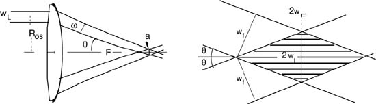
Fig.6-1 In an LDV, the laser beam is first collimated and divided into two parallel beams by the beamsplitter BS and folding mirror M. The beams are sent to the focussng lens L, with an off-axis shift R. The lens brings the beams to cross the axis at the focal distance F, under an angle tanθ=R/F. Horizontal fringes are formed at the beam crossover. The fringe spacing D is found setting the path length difference AB+AC equal to λ. A particle crossing the fringes at a speed v has brightness oscillating with a period T=D/v. The field scattered by the particle is converted by the photodetector in an electrical signal at a frequency v/D.

If we now expand the region of beam superposition (Fig.6-1, bottom) we can see that stationary fringes are formed. In fact, the loci of equal phase difference between the two wave fronts are horizontal planes, in the reference frame of Fig.6-1.

By drawing the wave front of the two beams, it is easy to derive the fringe spacing D. Let us go from point O on a fringe to point A in the next fringe, along the interfering beams. Considering first the beam k₁, we move along the wave front OB with no phase shift and then along BA perpendicular to the wave front with a path length delay D sinθ.

For beam k₂, we get with no phase shift along OC, and a path length delay -Dsinθ along CA.

Fig.6-2 Particles crossing the fringes in the superposition region (top left) with a velocity v (the y-component) develop an oscillating signal at frequency f_D=v/D, where D is the fringe spacing. The envelope of the oscillation replicates the Gauss distribution of the beam. Particle A, crossing the superposition region at the midpoint, develops the largest number of periods, and is the ideal response. Particle B gives fewer periods and its signal has less contrast. Particle C, outside the superposition region, only samples the beam distributions and its waveform carries no information.

The total path length difference of interfering beams is then 2 Dsinθ. By equating this quantity to λ for adjacent fringes, we get the fringe spacing as:

(6.1)

If a particle moving along the y-axis crosses the fringes with a velocity v, then it is illuminated by alternate bright and dark fringes, with a period T=D/v (Fig.6-1). The particle scatters radiation outward (see Appendix A3), and we can collect scattered power by a lens and photodetector combination (Fig.6-1), which provides an electrical signal for subsequent processing. The electrical signal contains information on velocity in form of the frequency of the oscillations developed by fringe crossing in the superposition region. The frequency is given by:

(6.2)

The envelope of the signal is a Gaussian distribution, a replica of the beam spatial profile of interfering beams.

As we can see in Fig.6-2, not all the particle positions are equally good to develop the Doppler signal, however. Particle A at the middle of the superposition region will cross the largest number of fringes and develop a clean oscillation with a Gaussian envelope. Particle B is halfway between the middle and the border of the superposition region and crosses half as much fringes, and in addition passes through a portion of the each beam alone. Thus, particle B develops fewer cycles, has a long Gaussian tail, and its oscillation has nonunity modulation depth because of beam intensity unbalance. Particle C is just outside the border of beam superposition and crosses no fringes. Thus, particle C develops a sample of the beam profile intensity instead of the desired Doppler signal. In the processing of signals, particle A has the best and most desired waveform, B is marginally useful, and C is to be discarded.

Returning to Eq.6.2, we can see that, in the laser Doppler velocimeter, the fluid velocity measurement is brought to a frequency measurement on the electrical signal, with a scale factor given by R= f_D/v= 2sinθ/λ[Hz/(m/s)].

This circumstance is very favorable, because it is well known that the frequency measurement is the best we can perform in electronics. It may cover 9 to 12 decades, from mHz or μHz to GHz and above. With a single counter circuit, we may easily perform a frequency measurement on 8 decades, for example from 1 Hz to 100 MHz. In addition, a frequency meter can be easily traced to standards of frequency, and the result is that our measurement has also a precision, not only accuracy, with typical values of Δf_D/f_D≈10^-6 and better.

Returning to the frequency measurement, let us consider the typical values of the scale factor R and of the velocity range we can attain. Using λ=0.633 μm and θ= 0.1 (5 deg)…0.5 (30 deg), we get R= 0.3…1.6 MHz/(m/s).

Because the angle dependence is not that strong, let us take R= 1 MHz/(m/s) as a reference value. This figure means that we can go from very small velocity, ≈μ/s, in the low range of frequency (Hz’s) to very high velocity, up to ≈100m/s, in the high range of frequency (100MHz’s). The wide span of frequency becomes translated in the wide span of velocity we can measure with the laser Doppler velocimeter.

6.1.1 The Velocimeter as an Interferometer

We can now show that the following descriptions of the velocimeter signal are equivalent: (i) the fringe crossing; (ii) the Doppler effect; and (iii) the interferometric phase shift.

About fringe crossing, the result of the analysis is Eq.6.2 we have already considered.

About the Doppler effect, it is well known that the frequency deviation Δf_D experienced when the source moves with respect to the observer at a speed v is Δf_D/f_D =v/c, or Δf_D=v/λ. Around the direction of illumination (Fig.6-1), the particle is seen to approach by one beam (k₁), and remove by the other beam (k₂). Then, considering that the obliquity factor is sinθ, we have Δf_D=v sinθ/λ and Δf_D=-v sinθ/λ for the two beams.

In conclusion, the total frequency difference is 2v sinθ/λ, the result of Eq.6.2.

Third, we can use the interferometric phase shift to derive the equivalence to Eq.6.2. When a field E₀ impinges on the particle from direction k₁ and we look it from direction k₀,

the field is given by:

E₀ exp i(k₁-k₀)· s

This expression is recognized as the generalization of the usual term E₀ exp 2ks, to the case of different directions of illumination and observation, where s is the displacement vector, and the dot “·” means scalar product.

We have two fields of illumination in the LDV velocimeter, k₁ and k₂. Therefore, the total field observed from direction k₀ is:

E = E₀ exp i(k₁-k₀)·s + E₀ exp i(k₂-k₀)·s

The signal found at the detector is proportional to the square modulus of the field, I ∝ |E|². Developing the modulus, we easily get:

I ∞ E₀²2 + E₀² 2 cos [(k₁-k₀)·s - (k₂-k₀)·s] = 2E₀²[1+ cos (k₁-k₂)·s]

Except for a constant term, the signal depends on the scalar product of the displacement s and the vector difference k₁-k₂ of the illuminating beam. Note that the result is independent from the observation vector k₀.

With the aid of Fig.6-3, it is easy to see that the difference k₁-k₂ is parallel to the y-axis (the vertical axis in Fig.6-2), and its modulus is given by (see Fig.6-3):

|k₁-k₂ |= 2k sin θ.

Fig.6-3 The vector difference of the illuminating wave vectors k₁ and k₂ is the argument of the phase shift φ =(k₁–k₂)·s observed for a particle under a displacement s.

For a particle making an in-plane displacement s parallel to the y-axis, the phase of the cosine function is then φ =(k₁–k₂)·s = 2ks sin θ. By time differentiating the phase shift φ, we obtain angular frequency (or pulsation) ω=2πf. Using the expression of φ, we can obtain frequency as:

f = (2π)^-1(dφ/dt) = (2π)^-12k(ds/dt) sinθ = 2 sinθv/λ

The result coincides with Eq.6.1 once more, and this demonstrates the equivalence of the Doppler effect and interferometric phase shift descriptions.

Fig.6-4 Top: An LDV configuration named ‘referenced’ because the photodetector is positioned to collect one of the illuminating beams and thus acts as the local oscillator for the homodyne detection of the fringe signal. Bottom: Another referenced configuration uses a beam deviated from the laser to the detector. Though fringes are not formed, the vector difference k_ill-k_obs determines the axis of sensitivity to the speed component.

Two other configurations related to interferometric arguments are reported in Fig.6-4. The first one (top in Fig.6-4) is called referenced detection and is obtained by moving the detector so that it intercepts the portion of the upper beam passing beyond the fringes. This beam acts as the local oscillator beam of a coherent homodyne detection [4], with the result that sensitivity is much increased compared to the placement of Fig.6-1, that operates in the direct detection regime.

The configuration is sensitive to the optical phase shift (k_ill-k_obs)·s, that is, to the velocity component along the vertical axis in the drawing of Fig.6-4.

This circumstance is no surprise because two interfering beams are in the superposition region that generates the usual horizontal fringes, like in the setup of Fig.6-1. The only basic difference with Fig.6-1 is the presence of the reference beam.

The second configuration in Fig.6-4 (bottom) is truly different from the previous ones, conceptually. The reference beam is again present, but illumination is provided only by one beam, and no fringes are formed. This configuration, one proposed and experimented in the early times of LDV [3], is itself sensitive to the optical phase shift (k_ill-k_obs)·s.

A last comment is on the difference between velocimetry and vibrometry (Sect.4.6). As already pointed out, both are actually interferometers, and it makes no fundamental difference if we look at the frequency signal rather than the phase signal. The true difference is the direction along which the component of s or v is measured: parallel or perpendicular to the line of sight aimed to the measurement volume. Another less basic difference is that the LDV looks at a velocity of a fluid moving in front of it, whereas the vibrometer looks at small periodic displacements.

6.2 Performance Parameters

Let us now discuss the parameters of operation of the velocimeter and the layout options affecting performance. We deal here with issues such as accuracy of the velocity measurement, sampling volume, and effect of alignment errors. In next sections, we consider the electronic processing and the optical setup configurations.

6.2.1 Scale Factor Relative Error

The scale factor of the Doppler velocity measurement is R= f/v= 2sinθ/λ. The relative error of R, or ΔR/R, is the sum of the relative errors Δθ/θ and Δλ/λ (absolute values). Usually, the wavelength error is not a problem because λ is known to a very good accuracy, at least Δλ/λ≈10^-4 or better (see also App.A1).

The angle of beam crossing can be expressed as θ = atan R_os/F where R_os is the axial offset of the beams and F is the focal length of the objective lens in Fig.6-1.

F is usually known with a typical 10^-4 accuracy, whereas R depends on the position of beamsplitter and folder mirror. R_os can be measured to 10^-4 accuracy as well, but the long-term stability of mechanical mounts may limit the repeatability to probably a few 10^-3.

In conclusion, from the measured frequency, we may expect to go back to velocity v=f_D/R with an accuracy ΔR/R≈10^-3.

6.2.2 Accuracy of the Doppler Frequency

Several sources limit the accuracy of the measured Doppler frequency f_D. Let us now consider the ultimate accuracy, the one set by the information content in the waveform being measured.

As we have seen previously, several types of waveforms are generated by particles crossing the fringe region in Fig.6-2. The cleanest waveform is that generated by particle A at the fringe middle, and this waveform is likely the best for information content. Thus, we now take particle A as a reference for our considerations.

In crossing the beams, particle A is shone by a Gaussian distribution with spot size w_m (Fig.6-1). Therefore, the waveform s(t) of the signal scattered out to the detector is a sinusoidal function multiplied by a Gaussian envelope, or:

s(t) = sin 2πf_Dt exp -t²/2σ_t²,

where σ_t = w_m/v is the standard deviation of the Gaussian (or 1/e² half-width), and v is the speed of the particle.

By calculating the Fourier transform of s(t) [5], we find that the frequency spectrum of the Doppler signal is again a Gaussian distribution, centered at the Doppler frequency f_D, or:

s(f) = exp -[(f-f_D)²(2πσ_t)²/2]

In this expression, the standard deviation σ_f of frequency f_D is σ_f =1/(2πσ_t). Substituting σ_t=w_m/v in this expression gives σ_f=[2πw_m/(f_DD)]^-1, and by rearranging we get:

(6.3)

Here, we have let N_f =w_m/D for the number of fringes contained in w_m.

In conclusion, we have shown that the relative accuracy σ_f/f_D of the Doppler measurement is proportional to the inverse of the number N_f of fringes crossed by the particle. Of course, because it is v=f/R, the same result holds also for the relative accuracy of the speed measurement, σ_v/v = 1/(2πN_f).

In point A, the height w_m of the fringe region (Fig.6-1) and the number N_f of fringes are maxima, and therefore the relative error σ_f/f_D is a minimum. This confirms the initial assumption that point A is the best for accuracy.

Now, let us consider those particles crossing the fringes off the optimal point A. Even if we are able to get rid of waveform artifacts (Fig.6-2), the number of fringes N’ progressively decreases from the maximum N_f to zero at the crossing border (point C in Fig.6-2).

By repeating the above calculation, we find that the relative accuracy is still given by Eq.6.3, but with the actual number N’ of fringes (or periods of the Doppler waveform) in place of N_f. Thus, as the particle crossing gets farther away from the middle of the superposition region, accuracy gets worse and worse.

Then, it will be appropriate to make a selection of ‘good’ particles and discard ‘bad’ ones.

As described later in next section, this selection will be actually performed by means of an a-posteriori electronic validation, which is equivalent to the limit of the lateral offset of particles allowed in the measurement. If the selection restricts the particles to those crossing at least N/2 fringes, for example, the relative accuracy is intermediate between (2πN_f)^-1 and (πN_f)^-1.

The maximum number of fringes in the superposition region (particle A in Fig.6-2) is given by the ratio of radial offset R_os to the spot size w_L of the beams to be recombined:

(6.4)

This result is derived on next section in the case of a focusing lens, but has a general validity.

Last, let us consider what happens if the measurement is repeated on N_M particles. If we take the average value of N_M individual measurements, the relative accuracy of the measurement improves as 1/√N_M.

Combining the 1/√N_M factor and the σ_f/f_D∝1/N_f dependence, it is easy to see that the laser Doppler velocimeter can attain very low values of the relative error (in velocity), for example 10^-3 or less. The caution is here that Eq.6.3 is an ultimate limit for accuracy that is approached only after properly curing other systematic errors, for example, the unequal spacing of fringes (see Sect.6.2.4).

6.2.3 Size of the Sensing Region

With the aid of Fig.6-5, we can easily calculate the size of the sensing region determined by the beam superposition, where fringes are formed. This is the measurement region, also called the sampling region or volume of the LDV. A feature specific of the laser Doppler velocimeter is the small size (mm or less) of the sampling region. Together with the noncontact operation, this is a definite advantage of LDV compared with other instruments. Let w_L be the beam size produced by the beam expander and reaching the entrance of the focusing lens. In the focal plane, the beam is focused to a spot size w_f (Fig.6-5). We can find w_f by applying the invariance of the acceptance α=aω [4], which is the product of the area and of the solid angle through which the bundle of rays is passing. For a single-mode spatial distribution, acceptance is equal to λ²[4].

Because a =πw_f² andω=π(w_L/F)², we may apply the previous statement and write for the spot size:

aω = πw_f²π(w_L/F)²= λ²

Solving this expression for w_f, we obtain:

Fig.6-5 The sensing region is defined by the longitudinal and transversal sizes, w_m, and w_l. These quantities depend on beam size w_L and offset radius R_os.

(6.5)

Now, we can take into account the obliquity factor (Fig.6-5, right) connecting the spot size to the transversal size w_m (a factor 1/cosθ) and to the longitudinal size w_l (a factor 1/sinθ). Doing so, we can write the following results:

(6.6)

In these expressions, the angle θ is determined by the offset radius R_os (Fig.6-5, left), and is given by R_os/F= tan θ.

Recalling the fringe spacing D=λ/2sinθ from Eq.6.1, we can work out the number of fringe as:

N_F= w_m/D = (πcosθ)^-1λF/w_L[λ/2sinθ]^-1= (2/π)tanθ F/w_L= (2/πR_os/w_L

The last term in the expression coincides with the result of Eq.6.4.

To illustrate the typical values that can be found in a velocimeter, we may consider the case R_os= 50mm and F = 200mm, calling for a lens with a diameter D_lens = 2R_os= 100mm (and with an F-number [4] F/=0.5).

The angle of superposition is found from R_os/F =tanθ= 0.25, as θ= 14°.

With a laser spot size w_L= 1mm on the focusing lens, we obtain a number of fringes N_F=(2/π)50-31.

The accuracy of the single velocity measurement is therefore σ_v/v=σ_f/f_D=(2πN_f)^-1=0.5%.

At the He-Ne wavelength λ=0.633μm, the fringe spacing is evaluated as D= 0.633μm/2·sin14°= 1.30μm, and the scale factor is R= 2sinθ/λ= 0.766 Hz/(μm/s) or, if preferred, 0.766 kHz/(mm/s) or MHz/(m/s). The focused spot size is w_f= (0.633μm) 200/π·1= 40μm. The sizes of the sensing region are: w_m= w_f/0.97= 41μm, and w_l= w_f/0.24 = 166μm.

As we can see, these central design values provide a good intrinsic accuracy and a small sampling volume. The sampling volume is not so far away from the focusing lens, however.

If we need to sense the fluid farther away, we may use a larger focal length, for example F=500mm. With this new value, the angle of superposition is tan θ= 0.1, or θ= 5.7°. With the same laser beam size w_L, the number of fringes is unchanged, as well as the accuracy σ_v/v. Fringe spacing and scale factor are increased to D=3.16μm, and R= 0.316 Hz/(μm/s). The focused spot size changes to w_f=(0.633μm) 500/π1= 100μm, and the sizes of the sensing region become w_m= w_f/0.995= 101μm, and w_l= w_f/0.1= 1000μm. Should this large value of the longitudinal size w_l be inconvenient, we can always trim it by the a-posteriori validation of fringe (see Sect.6.3.1).

6.2.4 Alignment and Positioning Errors

Errors in alignment of the beams sent to the focusing objective have the consequence of distorting the fringes in the superposition region.

As illustrated in Fig.6-6, an angular error of the parallelism of the beams results in an unequal spacing of fringes, whereas an unbalance of the lateral offset radius R tilts the fringes with respect to the optical axis.

Fig.6-6 At the focusing objective, errors of the incidence angle or of the lateral offset of the two beams result in fringes with unequal spacing (bottom left) or with a tilt with respect to the optical axis (bottom right).

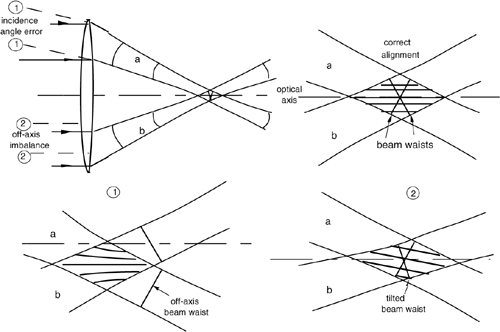
Of course, there are several other possible types of alignment or positioning error. All of them result in a specific distortion of the fringe pattern. Therefore, accuracy of the velocity measurement is reduced. To minimize the effect of alignment or positioning errors, we should employ an optical configuration that is easy to trim and mechanically stable in time. From this point of view, the configuration of Fig.6-1 is not the best because mirrors are affected by an angular error of their position, and each of them can go out of alignment.

A preferred configuration is shown in Fig.6-7 (left). Here, a cube beam splitter BS divides the incoming beam, and folding prisms are used in place of mirrors to derive beams b1 and b2. A prism, used as a mirror by the internal reflection at the 45° surface, is much sturdier and mechanically stable in time than a mirror on a flat. In addition, using the other two surfaces as a reference for the mechanical mount, the parallelism of P1, P2, and P3 is much easier to achieve. If desired, we could improve the configuration further with the use of Dove prisms as shown in Fig.6-7 (right).

Fig.6-7 Using a beamsplitter prism BS and the folding prisms P1-3 as mirrors (left), we obtain a splitting configuration much more stable and easily trimmed as compared with that of Fig.6-1. Even better, we can employ Dove prisms to minimize parts count and improve stability further (right).

A last interesting feature of the prism configuration is optical path-length balance. Looking at Fig.6-1, we can see that path lengths to the superposition region are different, because the lower beam reaches the lens straight, whereas the upper beam has the extra vertical path to cover. The difference is not so large, being of the order of 2R (typ. ≈100mm). However, if the laser source is multimode in frequency, that is, emits several longitudinal modes, we may face a reduction of the coherence factor.

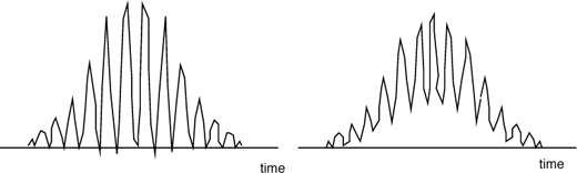
In this case, the fringe visibility is not a maximum and we get a sort of pedestal in the Doppler signal, as illustrated in Fig.6-8.

Using the prism configuration to generate the beam superposition, we enter parallel to the lens optical axis so that path lengths are balanced (Fig.6-7).

In addition to the configurations of Figs.6-1 and 6-7, several other variants have been proposed [3] and used in commercial LVDs.

Fig.6-8 The Doppler waveform has 100% modulation (or V=1 fringe visibility) if the two superposed beams have a path-length difference much less than the coherence length of the source (left). When coherence is not unity, or beams have unequal intensity, waveforms exhibit a pedestal (right).

6.2.5 Placement of the Photodetector

The photodetector collects the signal scattered out by the particle crossing the fringes and converts it to an electrical signal for processing. Because scattered light radiates in any direction, the photodetector could be in principle positioned everywhere around the beam crossing region. However, because we want to collect a large signal and the fluid flows in front of the objective lens, we have in practice just two options for the photodetector placement. As shown in Fig.6-9, we may place it beyond the fluid to look at the forward-scattered radiation or behind the objective lens to look at the backward-scattered radiation. In both cases, we will use an objective lens L’ to improve light collection and to define a certain solid angle of collection Ω.

In the two cases, at equal distance from the scattering volume and equal aperture of the objective lens, the signal collected is different because it is proportional to the value of the scattering function f(θ) (App.A3.1) in the forward (θ≈0) and in the backward (θ ≈π) direction, respectively.

The scattering function changes considerably when we go from the Rayleigh to the Mie regime. In the small-particle (rλ) Rayleigh regime, the scattering function is nearly iso-tropic, and then the forward-scattering and backward-scattering photodetectors are equivalent. However, we do not prefer working with very small particles, because the amplitude of the scattered signal, or the scattering cross section Q_ext(App.A3.1), is very small. Indeed, Q_ext is proportional to (r/λ)⁴ in the Rayleigh regime.

If the particle radius is comparable to wavelength or larger, we are in the Mie regime, in which the cross-section factor is comparatively large (Q_ext≈2) and the scattered signal is much increased. In the Mie regime, however, the scattering function f(θ) is strongly peaked forward.

The ratio p(π)/p(0), proportional to the relative photodetected signals in the backward and forward directions, is in general strongly dependent on the particle characteristics, but usually lies in the range 10^-3 to 10^-2.

Clearly, in this case, we will prefer collecting the signal in the forward direction, if the placement of the detector beyond the fluid is accessible. If it is not, we shall work in the backward direction and will use a detector of increased sensitivity to compensate for the reduced signal amplitude.

In practice, both photomultipliers and photodiodes (pin and avalanche) are used according to the required sensitivity [4].

The amplitude of the signal supplied by the photodetector can be calculated as follows. Let P_L be the laser power, split in the two beams and recombined in the scattering volume. A particle crossing the scattering volume is illuminated with a power density P_L/w_l² and scatters out a total power P_ts =(P_L/w_l²)Q_extπr²(App.A3.1).

Denoting with f(θ_meas) the scattering function evaluated at the measurement angle θ_meas (=0 or π), the signal collected in the solid angle Ω is written as 4πP_tsf(θ_meas) Ω. Last, recalling that the photogenerated current is σ times the detected power, σ being the spectral sensitivity [4], we get:

Fig.6-9 Light scattered by the particle in the measurement region can be collected by a photodetector looking at the forward scattering (top) or at the backward scattering (bottom).

(6.7)

In most schemes considered so far, we have assumed using direct detection to avoid unessential complication.

Coherent detection can be employed as well, at the expense of some extra complexity in the optical setup, and it generally improves the sensitivity of photodiodes without internal gain. Coherent detection requires that a fraction of the outgoing laser beam be superposed to the scattered return on the photodetector. (see also Ch.7 of Ref.[4]).

An example of this arrangement has been already provided in Fig.6-4.

In addition, most direct detection schemes of LDV can be easily converted to coherent ones. For example, with reference to Fig.6-9, we can convert to coherent detection by these three steps: (i) removing lens L’ so that the returning beam comes out collimated from L, (ii) adding beamsplitter m’ so that part of the reference beam is superposed on the photodetector, and (iii) changing the folding mirror in a beamsplitter.

6.2.6 Direction Discrimination

As in any interferometer, in a single-channel LDV we cannot distinguish the direction of the velocity, or tell v from –v. Actually, few cases exist in which direction discrimination is necessary, for example, vortex study.

In these cases, we may use the configuration of Fig.6-10 where a Bragg cell is inserted on one of the two recombining beams. The Bragg cell is a frequency shifter based on the acousto-optical effect. If the frequency of the input beam is f, from the output of the Bragg cell we get a frequency f+Δf. The typical shift in the range Δf =20-100 MHz.

Let us now consider the superposition of the two beams (Fig.6-10). We may repeat the reasoning of Sect.6.1.1, modified to take account of the different frequencies of the two beams.

Fig.6-10 By adding a frequency shifter on the path of one of the beams of the velocimeter, we generate a moving fringe pattern in the measurement region and are able to discriminate the direction of velocity v.

The total field is given by:

E = E₀ exp i [2πft+(k₁-k_obs)·s]+ E₀ exp i [2π(f+Δf)t+(k₂-k_obs)·s]

The signal at the detector, I ∞ |E|² is given by:

I ∝ E₀² 2 + E₀² 2 cos [2πΔft + (k₁-k₀)·s - (k₂-k₀)·s] = 2E₀² [1+ cos 2πΔft+(k₁-k₂)·s]

By time differentiation of the phase in the cosine term, we obtain frequency as:

f = (2π)^-1(dφ/dt) = (2π)^-1(d/dt)[2πΔft +(k₁-k₂)·s] = Δf +2 sinθv/λ

The result tells us that the velocity dependent frequency, 2sinθ v/λ, is superposed to the frequency shift Δf. Thus, as long as 2sinθ v/λ<Δf, we can determine the sign of v.

We can interpret the frequency bias introduced by the Bragg cell as an upward movement of the fringe pattern. Indeed, the shift Δf corresponds to a fringe velocity v_fr= λΔf/2 sinθ

6.2.7 Particle Seeding

About particles generating the scattered signal, we can either have them already present in the fluid as unintentional contaminant or can seed them purposely in the fluid under measurement. The seeding operation is preferable if practicable, because we can choose the diameter best suited for generating a clean and strong signal.

Usually, seed particles are Latex spheres of calibrated diameter, typically a few microns. These spheres are available from polymer companies in a range of sizes, from submicron to tens of micrometer in diameter.

The diameter is chosen large enough to give a large scatter signal in the Mie regime, but small enough compared to the fringe period to avoid averaging of the illumination spatial modulation.

The concentration of the spheres is readily calculated by assuming no more than one particle at the time in the scattering volume, for the reasons seen in next section. In view of the random spatial distribution the particles, we may take 0.1 as the design value of the average number. Then, we may write the concentration (in number per unit volume) as C_N=0.1/V_meas= 0.1 tanθ/w_l³. The corresponding relative volume concentration (or particle dilution) is C_V=0.4 r³tanθ/w_l

³. Typical design values of C_V turn out to be ≈10^-5 to 10^-4, that is, very small.

These small values explain why we can easily find the fluid already disseminated by a lot of scattering particle. When concentration is much larger than the desired one particle per scattering volume, we have two possibilities. One is to clean the fluid by filtering and then artificially seeding it, the other is increasing the scattering volume and using signal processing techniques tolerant to multiparticle superposition.

6.3 Electronic Processing Of The Doppler Signal

There are two options for the electronic processing of the Doppler signal obtained from the photodetector: time-domain and frequency-domain processing.

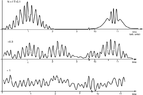
We prefer processing the waveform in the time domain when there is, on the average, much less than one particle at the time in the measurement volume, as in the case represented in Fig.6-11, top. Then, the output of the detector is a sequence of Gaussian-envelope oscillations, well distinct and separated in time. Each oscillation indeed carries a lot of information.

As we have found in Sect.6.2.2, a waveform with N_f periods allows us to measure frequency or velocity with a relative error Δf_D/f_D=Δv/v=1/2πN_f. There are also ‘poor’ waveforms with low N_f due to particles crossing near the edge of the fringe region, but these can be easily discarded by electronic processing in the time domain.

When the particle concentration increases, first we have the superposition of waveforms (Fig.6-11, middle), but the Gaussian envelopes can again be recognized. Then, we could still use time-domain processing, and wait for those waveforms that occasionally come isolated.

At a further increase of particle concentration (Fig.6-11, bottom), we cannot resolve individual waveforms any more and must revert to a frequency-domain method. With this method, we will look at the average frequency contained in the random-like superposition of Gaussian-envelope oscillations.

Fig.6-11 According to the average number N=fT of particles in the measurement volume, the waveform is best processed in the time domain (top) or in the frequency domain (bottom)

6.3.1 Time-Domain Processing

We assume that waveforms are distinct in time and do not overlap so that the periods contained in the waveform are well correlated to the frequency f_D=v/D.

Basically, the approach used to perform the velocity measurement follows the one outlined in Fig.6-12.

First, we perform a low-noise preamplification of the photodetector output signal and make available a clean Doppler waveform S(t). Then we time-differentiate S(t) so that eventual pedestal or slow drifts are canceled out. In the waveform S’(t) (Fig.6-13), the periods of oscillation are centered around the zero level and last 1/f_D. Next, we pass the signal through an amplitude discriminator with a threshold S₀ close to zero and obtain a square-wave signal S_SW that contains a number of periods N_f≈w_L/D equal to the number of crossed fringes.

Frequency f_D is determined by two counters, enabled by the presence of the Doppler signal S(t). To form the enable command, we make the envelope of S(t), obtaining S_env (Fig.6-13) and pass it through a discriminator with threshold S₀ (Fig.6-12). The result is S_enabl, a signal lasting a time T_C, which enables the gates to open the counters.

During time T_C, a main counter counts the number of periods N_f, and, simultaneously, an auxiliary counter counts the N_C pulses of a clock running at a suitable frequency f_C (Fig.6-12). The counts of the signal are N_f= f_DT_C and those of the clock are N_C= f_CT_C. By taking the ratio of the counts, we get a quantity V= N_f/N_C= f_D/f_C proportional to f_D= v/D.

Fig.6-12 In the time-domain processing, the Doppler signal is first time-differentiated and then squared by a discriminator with a threshold near to zero. Another discriminator works on the signal envelope to determine the presence of the signal and to enable the counters. One counter is for the Doppler signal periods, and the other is for the clock. When the signal is ended, an inspection circuit compares the counter content to the reference minimum. If content is high enough, the result is validated and passed on to calculate velocity, whereas if it is low, it is discarded.

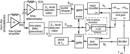
Fig.6-13 Waveforms in the time-domain processing. First diagram is the Doppler signal S(t) at the photodetector output. Second: Computing the time derivative S’(t), we are able to cancel out any pedestal and drift and get the Doppler frequency in form of zero-crossings. Third: After discrimination with a threshold S₀, we get N_f pulses in the time duration T_c. Signal end is obtained by an envelope detector, and yields a gate square wave lasting a time T_c. When signal is over, N_f is validated by an inspection circuit to stay within the expected limits of good signals. Clock pulses (N_c) are counted during T_c. By computing the ratio N_f / N_c, velocity is obtained.

We can also adjust the clock frequency so that the ratio v/f_CD is a decimal in the velocity v.

At the end of the signal, after Senabl has returned to zero, an end-of-pulse sequencer gates the division operation (Fig.6-12) and resets the counters for the next Doppler signal S(t). When a ‘poor’ Doppler signal is received, as exemplified by the second waveform in Fig.6-13, the number of counts N_f is low, and the content-check circuit of Fig.6-12 rejects the result at the end of computing period. This operation is carried out by digital comparators and registers of minimum/maximum counts (Fig.6-12). If N_f>N_min and N_f<N_max, the waveform is validated, and the content is passed on to the subsequent processing.

The minimum threshold N_min is usually set at half the maximum number of fringes N_f. This is a good compromise between accuracy of the single measurement and waste of useful data. With the threshold placed at N_f/2, all particles crossing the fringe region farther than half the longitudinal width w_l (Fig.6-5) are discarded. Therefore, the actual measurement volume is determined by a longitudinal size w_l/2. About the upper threshold N_max, this is set to a little bit more than N_f (for example 1.2N_f) to avoid taking two successive particles for one.

After the validation, the data processing may proceed in two ways, according to the type of measurement we are carrying out. If we deal with a single point measurement, for best accuracy, we will integrate the results of N successive measurements and exploit the 1/√fN dependence.

If we are measuring a velocity profile, we will use one or a few measurements and then move to the next point of the scan, either along a line or in a raster pattern. A line scan is readily accomplished by translation of the focusing lens, which moves the measurement volume axially. A raster scan or a more complicated pattern will require a suitable moving mirror arrangement.

6.3.2 Frequency-Domain Processing

When particles crowd up the measuring volume as in shown in Fig.6-11 bottom, time-domain processing can no longer be used. The signal oscillations carrying the Doppler frequency are damped out in amplitude and have a frequency jitter. In this case, given an average number N1 of particles in the measuring volume, the signal exhibits amplitude and phase fluctuations resembling those of the speckle pattern.

Indeed, the total signal is the summation of the contributions of N particles, and each particle yields a waveform of the type shown in Fig.6-11, top. Because the time of occurrence of each particle is randomly distributed, we have a summation of N uncorrelated contributions. The result is a field that replicates, for high N, the speckle pattern statistics, with zero mean value of the phase and quadrature components. Consequently, the intensity distribution is a negative exponential with a decay constant equal to the mean value.

It is then clear that, should we attempt a time-domain processing, the number of counts N_f per period T_c will be affected by a large error.

More appropriately, we shall look directly at the frequency content of the signal S(t), as obtained at the output of the preamplifier stage following the photodetector.

There are two approaches for frequency-domain processing: autocorrelation, and phase-locked loop.

In the first approach, we compute the autocorrelation function c(τ) = ∫_0-∞ S(t)S(t+τ) dt. The calculation can be performed by converting the signal S(t) to digital, with the aid of an Analog to Digital Converter (ADC), and then acquiring the data and computing c(τ) numerically in a computer unit.

The ADC does not need a very high resolution (usually, 8 bits will be adequate) because the round-off error is usually small respect to that of waveform noise. Rather, the ADC and the acquisition interface need to be fast if we are to cover the high-velocity range allowed by the LDV instrument (see Sect.6-2). For example, if we get 100 kHz of conversion and acquisition rate, we are then bound to a maximum velocity v≈1μm·100kHz= 0.1 m/s.

From the autocorrelation function c(τ), we may already obtain the velocity by looking at the first zero of c(τ). If c(τ)=0 for τ=τ_z, then the main frequency contained in S(t) is f=1/τ_z. Alternatively, we may compute the Fourier transform of c(τ), for example by means of a FFT algorithm that will be easily available if we are using a personal computer for acquiring S(t) and computing c(τ). Because of the well-known Wiener-Khintchine theorem [5,6], the transform of c(τ) is the power spectrum of the signal S(t). Thus, the power spectrum is a well-defined line at the Doppler frequency f_D if the fluid has a uniform velocity or is a distribution p(f) of spectral content if the fluid has a distribution of velocity.

When velocity is very high and the signal S(t) has a frequency content too high for the ADC and interface, we can resort to a second approach based on the PLL technique. As shown in Fig.6-14, the signal S(t) at the preamplifier output is compared to the oscillation of a Voltage Controlled Oscillator (VCO). The phase error is used to correct the frequency of the VCO until it is dynamically locked to the frequency of the Doppler oscillation contained in S(t). The gain and filter sections following the phase discriminator act as the feedback loop of the frequency-tracking operation. With them, we can filter signal S(t), which may vary in frequency, yet keep a narrow band around the average frequency, which results in a very effective cleaning-up of the signal.

Fig.6-14 The Doppler signal of an LDV can be filtered for f_D extraction by a simple PPL (phase locked loop) arrangement.

6.4 Optical Configurations

Lot of configurations have been experimented with through the years and reported in the literature. Several of them have gained acceptance for specific applications and are incorporated in commercially available products.

Fig.6-15 LDV configurations incorporated in products. From top to bottom: (i) forward-looking configuration ending on a photomultiplier; (ii) backward configuration; (iii) two-components LDV using a two-lines Ar-ion laser; (iv) fiber optics configuration that connects the laser and the receiver sections to the measuring volume (by courtesy of Dantec Dynamics, Copenhagen).

As we can see in Fig.6-15, we have a forward-looking LDV (first line in Fig.6-15) that uses a He-Ne laser as the source and an S-20 photomultiplier (see Ref.[4], Ch.4) as the detector. This is the simplest and probably the cheapest configuration of LDV. The same arrangement, but designed to collect the back-scattered signal, is shown in the second line of Fig.6-15.

As already pointed out, the forward-scatter configuration collects a larger optical signal compared to the backward-scatter one, but of course can be used only if we are allowed to access the region under measurement from two opposite sides. If we cannot do that, then we shall use the backward-scatter configuration.

The third line illustrates a dual-component (v_x and v_y) measurement of the velocity field, developed with a dual-λ Ar-ion laser emitting at 488 and 514 nm. The beams at the two wavelengths are separated by an interference filter, and then are directed to two beamsplitter-and-mirror combinations arranged along the x- and y-axis. Thus, at the focusing lens, we find two pairs of beams arranged in perpendicular planes. The measurement volume is thus illuminated with a double pattern of fringes, in the planes xz and yz, sampling the components v_x and v_y of velocity.

The same λ-selective operation is carried out in the backward path. Light collected by the objective lens comes to an interference filter oriented at 45 degrees, so that the beam at one wavelength is reflected and the other is transmitted. The detector section is duplicated to sort the velocity signals separately out along the x-axis and the y-axis.

The last line depicts a fiber optics version of the LDV. Here, source and detector are optically delivered to the superposition volume by means of a bundle of optical fibers.

These fibers are usually multimode to provide a large acceptance surface for the returning optical field. This maximizes the collected signal, but may impair the spatial coherence of the beams to be superposed in the measurement region.

A refinement is to use a single-mode fiber for the downlead path, so that the single-mode spatial distribution is preserved, and surround the single-mode fiber with an annulus of multimode fibers, so that collection of scattered field is maximized.

All the instruments described in Fig.6-15 are based on the external configuration of the interferometer (Sect.4.5). However, we can also envision using the other two configurations described in Sect.4.5 as well.

The internal configuration is outside this discussion because of the high attenuation suffered in the back-scattering path, preventing oscillation of the laser.

The self-mixing configuration can be used, and it has been reported in the literature [7,8] as an example of applying the injection concept since the early experiments. Some of the papers reporting a self-mixing velocimeter were actually on what we have called a vibrometer (Sect.4.6). That is, some of them described an instrument providing the v_z component of the target motion (the z-axis being the line-of-sight) and operating on a surface rather than on particles dispersed in a fluid.

To have a true velocimeter (or LDV) measuring the out-of-plane (v_x or v_y) velocity component, we will start with a laser with a good self-mixing effect and add an appropriate optical section. This section will be composed of the usual beamsplitter, mirror, and objective lens arrangement shown in the basic schematic of Fig.6-1. In this configuration, the field returning from the scattering volume is collected by the objective lens and fed into the laser cavity.

Here, the injection generates the usual AM- and FM- induced modulation. If we limit ourselves to detect the easy amplitude modulation component, it will suffice to place a photodetector on the rear mirror of the laser to get the desired LDV signal.

Of course, the self-mixing LDV can only operate in the backward-scatter configuration. Compared to the external interferometer configuration, there is the extra loss of mirror transmittance, but the optical part count is the minimum possible.

References

[1] Y. Yeh and H.Z. Cummins, “Localized Fluid Flow Measurements with a He-Ne Laser”, Appl. Phys. Lett. vol.4 (1964), pp.176-178.

[2] S. Donati, “Electro-Optics in the year Y2K”, web paper at http://ele.unipv.it/^∼ donati.

[3] L.E. Drain, “The Laser Doppler Technique”, J. Wiley and Sons: Chichester, 1980.

[4]. S. Donati, “Photodetectors”, Prentice Hall: Upper Saddle River, 2000.

[5] J.D. Gaskill, “Linear Systems, Fourier Transforms and Optics”, J.Wiley and Sons: New York, 1978, Chapter 7.

[6] M.J. Buckingham, “Noise in Electronic Devices and Systems”, Ellis Horwood: Chichester, 1983.

[7] M.J. Rudd, “A Laser Doppler Velocimeter Employing the Laser as a Mixer-Oscillator”, Journal of Physics E, vol.1 (1968), pp.723-726.

[8] P.J. de Groot, G. Gallatin, and S.H. Macomber, “Ranging and Velocimetry Signal in a Backscattering Modulated Laser Diode”, Applied Optics, vol.27 (1988), pp.4475-4480.